2. Materials and Methods
2.2. Modeling
To increase uniformity for ease of comparison while maintaining a robust search for well-performing models, we employed Autosklearn2.0 [
18,
19]. This meta-model has a search space consisting of every model within Scikit-Learn and subsequently searches over hyperparameter space per model. The training is conducted on four CPUs, 26 GB of RAM, 3 h of training time, 6572 MB of memory per job, log loss as the objective function, and no limit to the number of models on disk.
We compare the following six imputation methods alongside an oversampling preprocessing step.
No Imputation: This method involves not performing any imputation on the dataset, leaving the missing values as they are. In this approach, the model chosen must inherently be capable of handling missing data. Techniques such as decision trees or certain ensemble methods can often process datasets with missing values directly. This method is based on the assumption that the model can interpret and manage the missingness in the data without any explicit intervention.
Automatic Imputation (via Autosklearn): This approach employs Autosklearn, an automated machine learning tool, to determine the best imputation method for the dataset. Autosklearn explores various imputation strategies as part of its preprocessing pipeline and selects the one that optimizes model performance. This method leverages the power of automated machine learning to identify the most effective imputation technique, which could range from simple strategies like mean or median substitution to more complex ones, based on the characteristics of the data.
Constant Fill: In this approach, missing values are filled with a constant value. This constant could be a number outside the normal range of values (such as −1) to differentiate imputed values from real ones. The advantage of this method is its simplicity and the clear demarcation it provides, which can be helpful in certain analytical contexts.
Mean Substitution: Mean substitution involves replacing missing values in a dataset with the mean value of the respective column. This method assumes that the missing values are randomly distributed and that the mean is a representative statistic for the missing data. It is a straightforward approach but may not always be suitable, particularly in cases where the data distribution is skewed or the mean is not a good representation of the central tendency.
Median Substitution: Similar to mean substitution, median substitution replaces missing values with the median of the respective column. This method is particularly useful in datasets where the distribution is skewed or there are outliers, as the median is less affected by extreme values than the mean. It is a robust approach that can provide a better central tendency estimate in certain types of data distributions.
Multiple Imputation with Bayesian Ridge: This is a more sophisticated approach where multiple imputation is performed using Bayesian Ridge regression. In this method, missing values are estimated based on observed data, with the Bayesian Ridge regression model used to predict the missing values. Specifically, one begins by denoting one column of the training input f and the other columns . A Bayesian Ridge regression model is then fitted on . This is conducted for every feature and can be repeated so that in the next round, the previous rounds’ predictions can be used to make better predictions of the missing value. In this paper, we use 15 imputation rounds. The number of imputation rounds, 15, is chosen arbitrarily. The higher the number, the more accurate the imputation should be. For a dataset as large as All of Us, we chose to keep it lower. This technique considers the uncertainty in the imputation process by creating several imputed datasets and combining the results, leading to more accurate and reliable imputation compared to single imputation methods.
Each of these imputation methods has its strengths and weaknesses and is suitable for different types of datasets and missing data patterns. The choice of imputation method can significantly impact the performance of the subsequent analysis or machine learning models.
Random oversampling is a technique used to address class imbalance in a dataset, particularly in situations where the dataset has a disproportionate number of instances in different classes. This imbalance can lead to biased or inaccurate model performance, as the model may tend to favor the majority class.
In random oversampling, the idea is to balance the dataset by increasing the size of the underrepresented class (minority class). This is accomplished by randomly duplicating instances from the minority class until the number of instances in both the minority and majority classes is approximately equal. This method creates additional samples from the minority class not by generating new samples but by resampling from the existing samples.
In total, there are 12 different models to test with the same underlying classifier.
4. Discussion
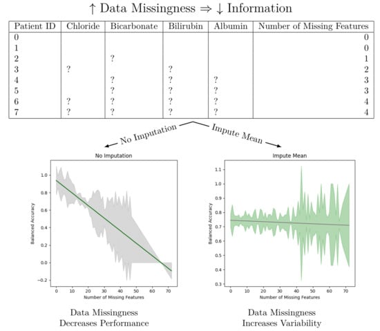
We observe that imputation methods homogenize the amount of information per patient. That is, without imputation, the models have a sharp performance loss, whereas imputation makes the slope less steep at the cost of increasing heteroskedasticity. We also note that every statistical test agrees between the oversampled and non-oversampled models. This trend underscores the sensitivity of predictive models to the method of handling missing data in electronic health records (EHR). The negative slope indicates that as the degree of imputation increases—implying more data are being estimated rather than observed—the accuracy, precision, and recall of the models tend to decrease. This phenomenon can be attributed to the fact that imputation, despite being a necessary process to address missing data, introduces a level of uncertainty or noise. This noise can distort the underlying patterns within the data, leading to less reliable predictions from the models.
We are not the first paper to study diabetes prediction using the All of Us dataset. A paper by Abegaz et al. studied the application of machine learning algorithms to predict diabetes in the All of Us dataset [
17]. Their work presents the AUROC, recall, precision, and F1 scores stratified by gender of the random forest, XGBoost, logistic regression, and weighted ensemble models. Our work builds upon those foundations in three ways. First, we note that all of the models in Abegaz et al.’s work can be found in Scikit-Learn. Hence, we performed a deep search over all Scikit-learn models to find the best performing ones. Second, we presented our results for further substrata of the dataset. One of the most important features of AoU is the diversity of people within the dataset. We highlighted the five performance metrics on the total testing dataset on each gender, on each race, and on groups bucketed by the number of missing features. We also presented the models’ performance on a number of fairness measurements when the sub-populations have a clear privileged group. Third, our largest deviation from the previous work was to show how the performance of a model changes as one changes the number of missing features.
The model performance in
Figure 1 and
Figure 2 has been trained for only three hours (as opposed to the multiday- or multiweek-long training that some deep neural network solutions provide) and yields modest results. Our best performing model is the “Auto Impute” model. We may compare the performance of that model to Abegaz et al.’s work. “Auto Impute” has a higher AUROC, comparable precision, and worse recall and F1. We note, however, that these are not clinically ready. Further improvements need to be made in order to prefer this to a HbA1c test for diabetes testing. Since the multiple imputer only used 15 iterations, the algorithm likely did not stabilize and caused the performance to drop. We emphasize that the primary objective of our research was not to maximize the performance of machine learning models applied to AoU data, but instead to study the effects of data missingness and imputation strategies on model performance.
Our analysis also highlights the presence of statistically significant heteroskedastic variance in model performances across imputation methods. Heteroskedasticity, in this context, refers to the irregular variability in the performance of predictive models, dependent on the amount and pattern of missing data being imputed. This irregular variance poses a significant challenge in predictive modeling, as it implies that the error terms (or the differences between predicted and actual values) are not uniformly distributed. Models thus exhibit different levels of accuracy and reliability depending on the specific characteristics of the missing data in each patient record.
The presence of heteroskedastic variance can be particularly problematic in clinical settings. It implies that for some patients, especially those with more extensive or particular patterns of missing data, the predictions made by the models could be less reliable. This inconsistency could lead to disparities in clinical decision-making, potentially affecting the quality of care provided to certain patient groups. Since the “Auto Imputation” model has the largest Y-intercept and one of the most negative slopes, it might be most beneficial to use the “Auto Impute” method for patients with few missing values in a clinical setting. For patients with a lot of missing values, one may use another imputation method with a less steep slope or perform a cost–benefit analysis of ordering more tests to make the model more performant.
These findings highlight the critical need for developing more robust imputation techniques that can minimize the introduction of noise and ensure uniform model performance across varying degrees of missing data. It also underscores the importance of considering the nature and pattern of missing data when applying machine learning models in healthcare settings. Future research should focus on exploring advanced imputation methods, possibly incorporating domain knowledge or utilizing more sophisticated algorithms, to mitigate the effects of data missingness on predictive model performance. In conclusion, while imputation is a necessary step in dealing with incomplete datasets for some models, our study indicates that current methods have significant limitations.
Addressing these limitations is crucial for the development of reliable and consistent machine learning models for clinical predictions, ultimately enhancing the quality of patient care and health outcomes. Our analysis on data missingness revealed that individuals who are male and persons of color would be disproportionately affected by a loss in performance with respect to data missingness. This is due to the number of missing features being more highly correlated with males and non-white people.
Future work can be conducted to ensure the robustness of the findings. A number of unanswered questions remain, such as: (1) does heteroskedasticity depend on certain features included in the model over another? (2) Do these findings pertain to more modern and complex deep learning models? (3) What other forms of data augmentation can be performed to reduce heteroskedasticity? Another comparison of interest is exploring whether the testing dataset holds more missing values than the training dataset and how the performance differs compared to the case of having roughly similar missing values between training and testing. If the testing dataset does not require many labels, then hospitals could save time and money by not measuring every missing value.
Author Contributions
Conceptualization, Z.J. and P.W.; methodology, Z.J.; software, Z.J.; validation, Z.J. and P.W.; formal analysis, Z.J.; investigation, P.W.; resources, Z.J.; data curation, Z.J.; writing—original draft preparation, Z.J.; writing—review and editing, Z.J. and P.W.; visualization, Z.J.; supervision, P.W.; project administration, P.W. All authors have read and agreed to the published version of the manuscript.
Funding
This research received no external funding.
Institutional Review Board Statement
Not applicable.
Data Availability Statement
Restrictions apply to the availability of these data. Data were obtained from the National Institutes of Health’s All of Us and are available at
https://www.researchallofus.org/ (accessed on 12 January 2024) with the permission of National Institutes of Health’s All of Us. Obtaining access to the data involves institutional agreement, verification of identity, and mandatory training.
Conflicts of Interest
The authors declare no conflicts of interest.
References
- World Health Organization. ICD-11: International Classification of Diseases 11th Revision: The Global Standard for Diagnostic Health Information; World Health Organization: Geneva, Switzerland, 2019. [Google Scholar]
- Cole, J.B.; Florez, J.C. Genetics of diabetes mellitus and diabetes complications. Nat. Rev. Nephrol. 2020, 16, 377–390. [Google Scholar] [CrossRef] [PubMed]
- Association, A.D. Diagnosis and classification of diabetes mellitus. Diabetes Care 2010, 33, S62–S69. [Google Scholar] [CrossRef] [PubMed]
- Group, T.S. Long-term complications in youth-onset type 2 diabetes. N. Engl. J. Med. 2021, 385, 416–426. [Google Scholar] [CrossRef] [PubMed]
- Rooney, M.R.; Fang, M.; Ogurtsova, K.; Ozkan, B.; Echouffo-Tcheugui, J.B.; Boyko, E.J.; Magliano, D.J.; Selvin, E. Global prevalence of prediabetes. Diabetes Care 2023, 46, 1388–1394. [Google Scholar] [CrossRef] [PubMed]
- Haw, J.S.; Shah, M.; Turbow, S.; Egeolu, M.; Umpierrez, G. Diabetes complications in racial and ethnic minority populations in the USA. Curr. Diabetes Rep. 2021, 21, 1–8. [Google Scholar] [CrossRef] [PubMed]
- Khanam, J.J.; Foo, S.Y. A comparison of machine learning algorithms for diabetes prediction. ICT Express 2021, 7, 432–439. [Google Scholar] [CrossRef]
- Hasan, M.K.; Alam, M.A.; Das, D.; Hossain, E.; Hasan, M. Diabetes prediction using ensembling of different machine learning classifiers. IEEE Access 2020, 8, 76516–76531. [Google Scholar] [CrossRef]
- Krishnamoorthi, R.; Joshi, S.; Almarzouki, H.Z.; Shukla, P.K.; Rizwan, A.; Kalpana, C.; Tiwari, B. A novel diabetes healthcare disease prediction framework using machine learning techniques. J. Healthc. Eng. 2022, 2022, 1684017. [Google Scholar] [CrossRef] [PubMed]
- Oikonomou, E.K.; Khera, R. Machine learning in precision diabetes care and cardiovascular risk prediction. Cardiovasc. Diabetol. 2023, 22, 259. [Google Scholar] [CrossRef] [PubMed]
- Anderson, J.P.; Parikh, J.R.; Shenfeld, D.K.; Ivanov, V.; Marks, C.; Church, B.; Laramie, J.; Mardekian, J.; Piper, B.; Willke, R.; et al. Reverse Engineering and Evaluation of Prediction Models for Progression to Type 2 Diabetes. J. Diabetes Sci. Technol. 2016, 10, 6–18. [Google Scholar] [CrossRef] [PubMed]
- Cahn, A.; Shoshan, A.; Sagiv, T.; Yesharim, R.; Goshen, R.; Shalev, V.; Raz, I. Prediction of progression from pre-diabetes to diabetes: Development and validation of a machine learning model. Diabetes/Metabolism Res. Rev. 2020, 36, e3252. [Google Scholar] [CrossRef] [PubMed]
- Ravaut, M.; Sadeghi, H.; Leung, K.K.; Volkovs, M.; Rosella, L. Diabetes Mellitus Forecasting Using Population Health Data in Ontario, Canada. arXiv 2019, arXiv:abs/1904.04137. [Google Scholar]
- Hudson, K.; Lifton, R.; Patrick-Lake, B.; Burchard, E.G.; Coles, T.; Collins, R.; Conrad, A. The Precision Medicine Initiative Cohort Program—Building a Research Foundation for 21st Century Medicine; Precision Medicine Initiative (PMI) Working Group Report to the Advisory Committee to the Director, National Institutes of Health: Bethesda, MD, USA, 2015. [Google Scholar]
- Sankar, P.L.; Parker, L.S. The Precision Medicine Initiative’s All of Us Research Program: An agenda for research on its ethical, legal, and social issues. Genet. Med. 2017, 19, 743–750. [Google Scholar] [CrossRef] [PubMed]
- Mapes, B.M.; Foster, C.S.; Kusnoor, S.V.; Epelbaum, M.I.; AuYoung, M.; Jenkins, G.; Lopez-Class, M.; Richardson-Heron, D.; Elmi, A.; Surkan, K.; et al. Diversity and inclusion for the All of Us research program: A scoping review. PLoS ONE 2020, 15, e0234962. [Google Scholar] [CrossRef] [PubMed]
- Abegaz, T.M.; Ahmed, M.; Sherbeny, F.; Diaby, V.; Chi, H.; Ali, A.A. Application of Machine Learning Algorithms to Predict Uncontrolled Diabetes Using the All of Us Research Program Data. Healthcare 2023, 11, 1138. [Google Scholar] [CrossRef] [PubMed]
- Feurer, M.; Eggensperger, K.; Falkner, S.; Lindauer, M.; Hutter, F. Auto-Sklearn 2.0: Hands-free AutoML via Meta-Learning. arXiv 2020, arXiv:2007.04074 [cs.LG]. [Google Scholar]
- Feurer, M.; Klein, A.; Eggensperger, K.; Springenberg, J.; Blum, M.; Hutter, F. Efficient and Robust Automated Machine Learning. Adv. Neural Inf. Process. Syst. 2015, 28, 2962–2970. [Google Scholar]
- Bellamy, R.K.E.; Dey, K.; Hind, M.; Hoffman, S.C.; Houde, S.; Kannan, K.; Lohia, P.; Martino, J.; Mehta, S.; Mojsilovic, A.; et al. AI Fairness 360: An Extensible Toolkit for Detecting, Understanding, and Mitigating Unwanted Algorithmic Bias. arXiv 2018, arXiv:1810.01943. [Google Scholar]
- Mehrabi, N.; Morstatter, F.; Saxena, N.; Lerman, K.; Galstyan, A. A survey on bias and fairness in machine learning. ACM Comput. Surv. (CSUR) 2021, 54, 1–35. [Google Scholar] [CrossRef]
- Caton, S.; Haas, C. Fairness in machine learning: A survey. ACM Comput. Surv. 2020. [Google Scholar] [CrossRef]
- Barocas, S.; Hardt, M.; Narayanan, A. Fairness and Machine Learning: Limitations and Opportunities; MIT Press: Cambridge, MA, USA, 2023. [Google Scholar]
- Speicher, T.; Heidari, H.; Grgic-Hlaca, N.; Gummadi, K.P.; Singla, A.; Weller, A.; Zafar, M.B. A unified approach to quantifying algorithmic unfairness: Measuring individual &group unfairness via inequality indices. In Proceedings of the 24th ACM SIGKDD International Conference on Knowledge Discovery & Data Mining, London, UK, 19–23 August 2018; pp. 2239–2248. [Google Scholar]
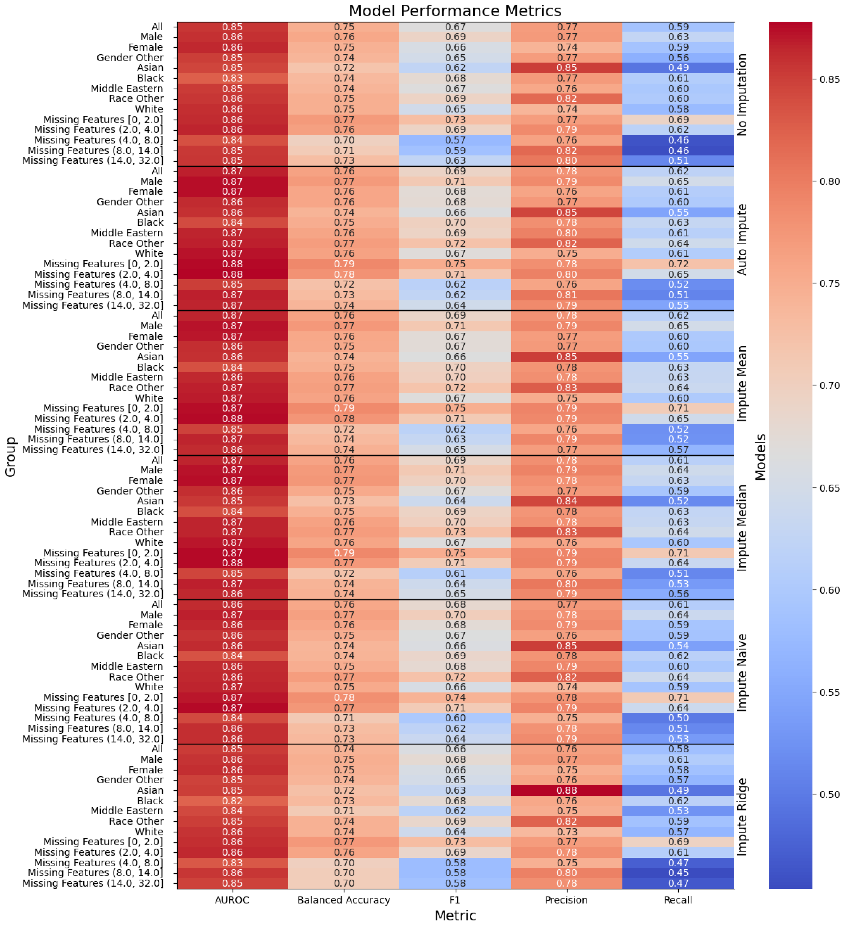
Figure 1.
Performance of the models, with the columns denoting the specific metric, across the evaluated sub-population (left label) and the imputation method (right label). The color denotes the magnitude of the metric, warmer colors indicating higher performance. The text color is adjusted to be readable given the background color.
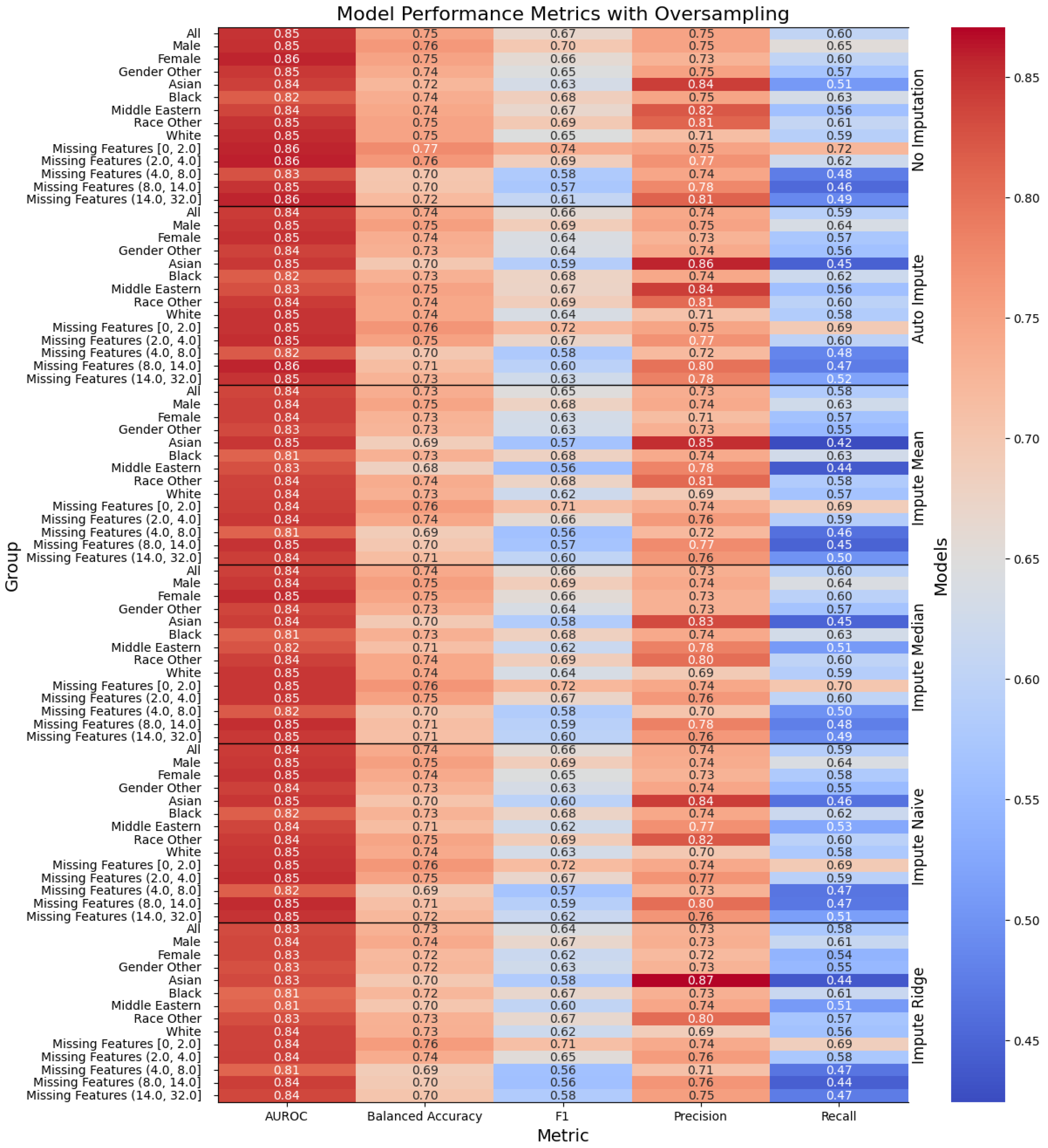
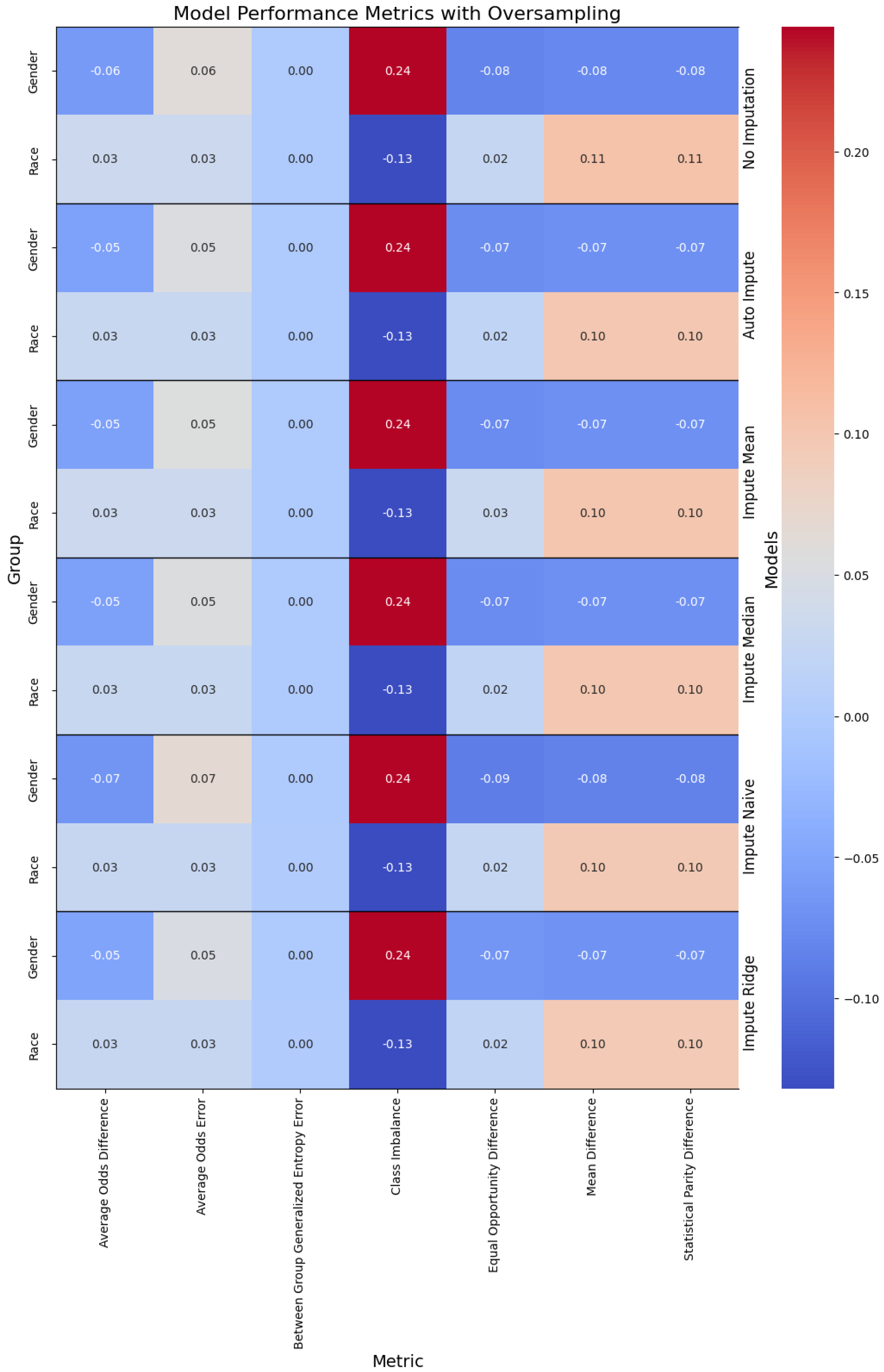
Figure 2.
Performance of the models when oversampling, with the columns denoting the specific metric, across the evaluated sub-population (left label) and the imputation method (right label). The color denotes the magnitude of the metric, warmer colors indicating higher performance.
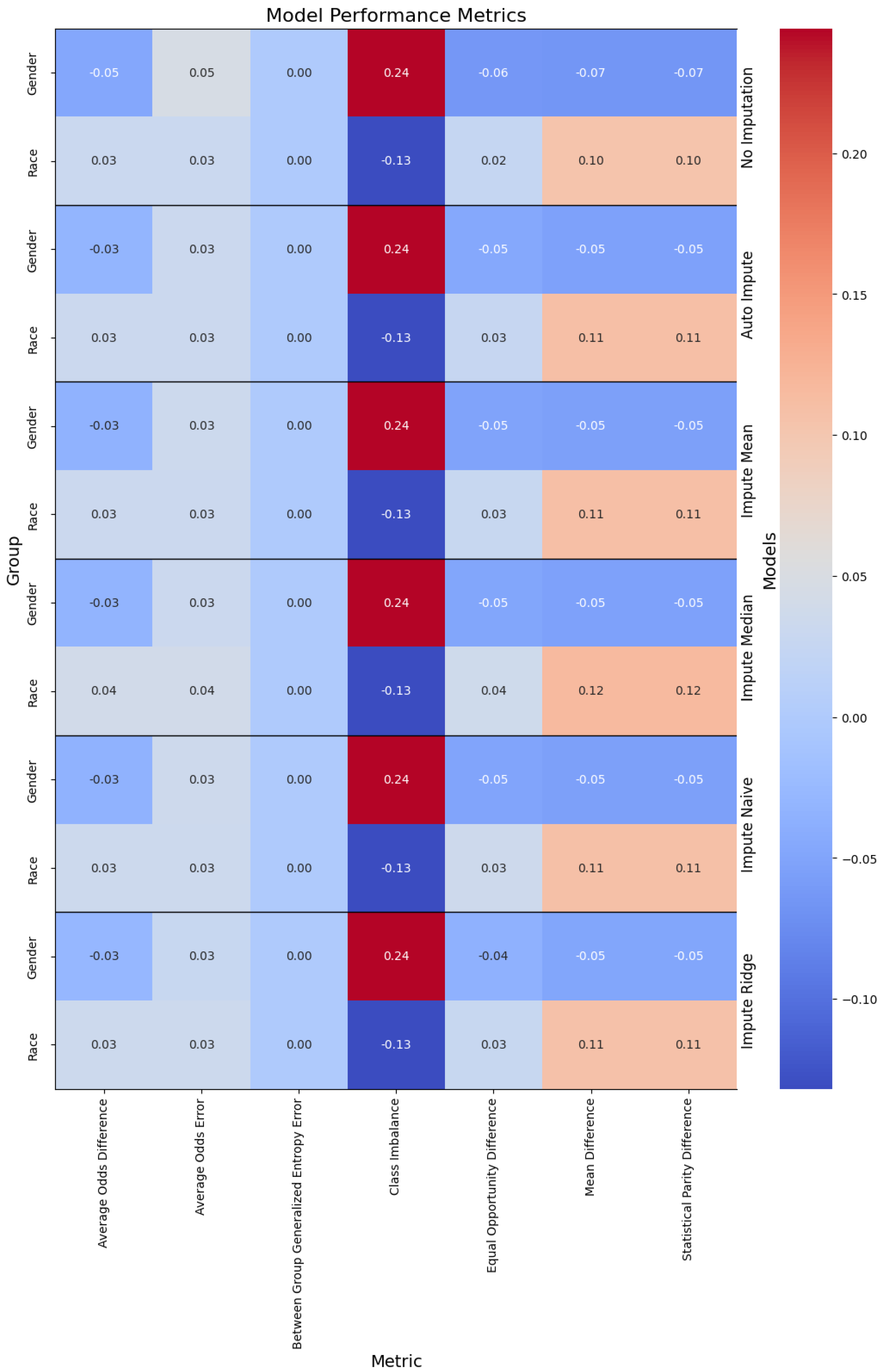
Figure 3.
Performance of the models, with the columns denoting the specific metric, across the evaluated sub-population (left label) and the imputation method (right label).
Figure 4.
Performance of the models when oversampling, with the columns denoting the specific metric, across the evaluated sub-population (left label) and the imputation method (right label). The color denotes the magnitude of the metric, with warmer colors indicating better performance. The text color is adjusted to be readable given the background color.
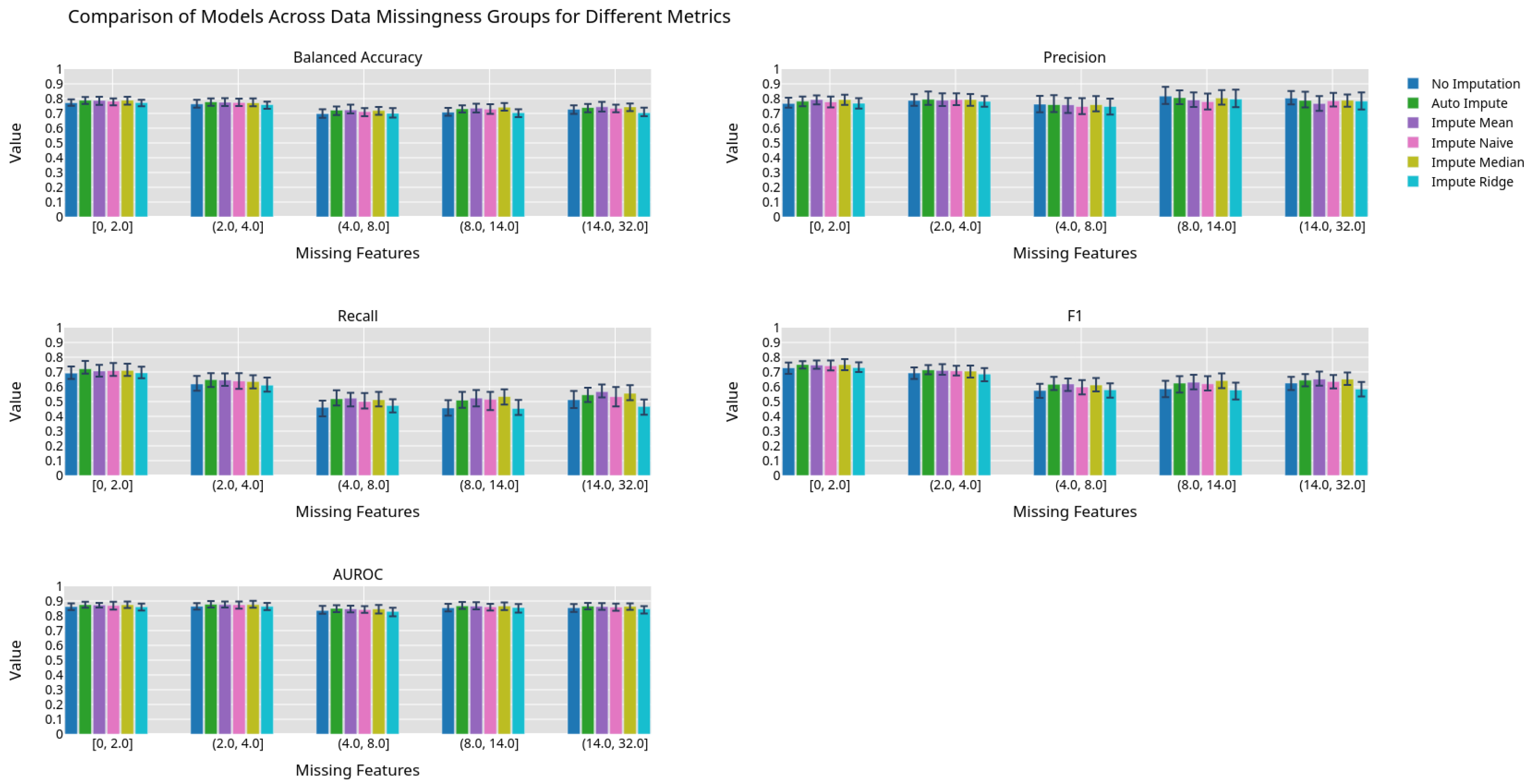
Figure 5.
Machine learning performance exhibited by different imputation methods grouped by 0.2 quantiles.
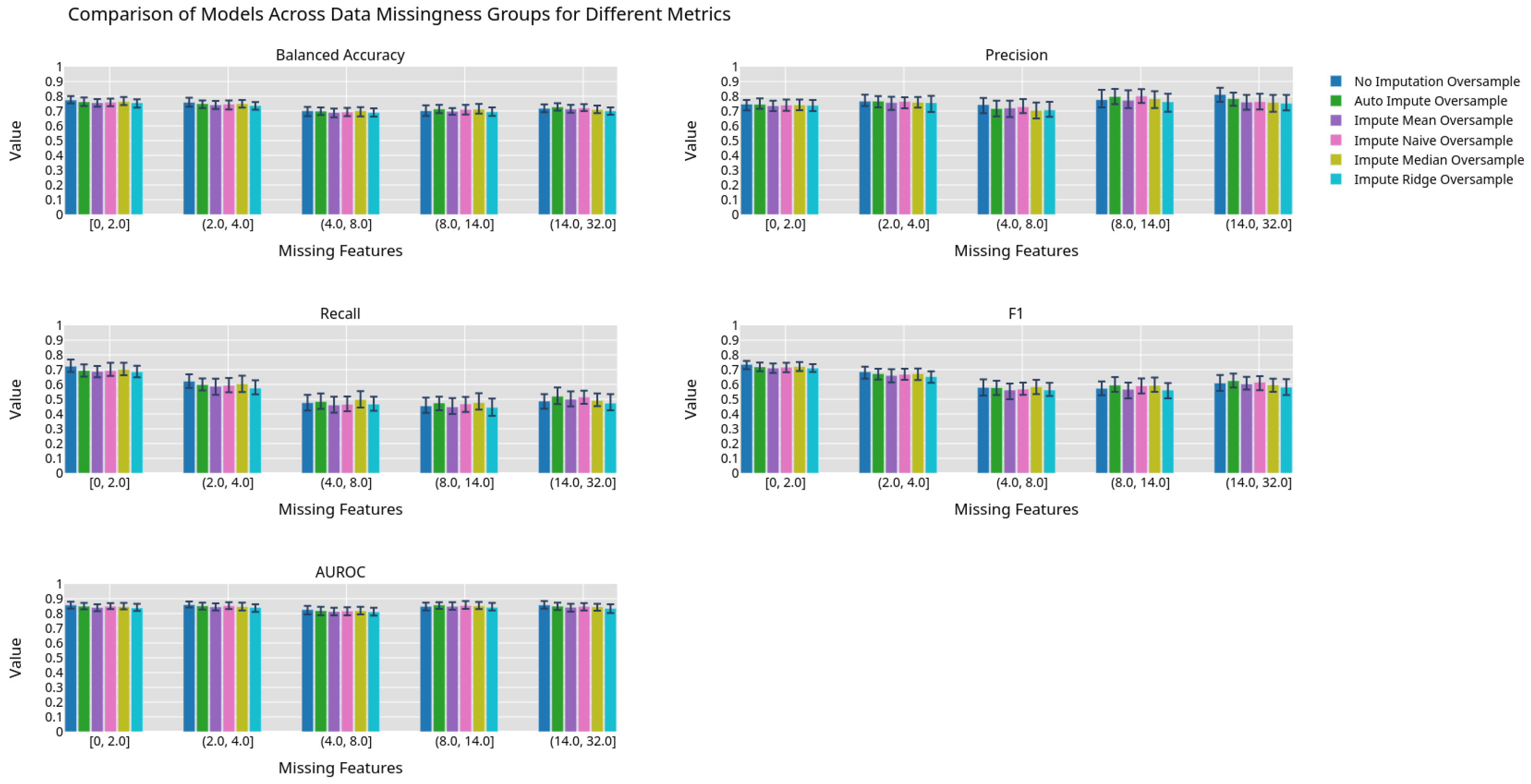
Figure 6.
Machine learning performance exhibited by different imputation methods using an oversampling preprocessing step grouped by 0.2 quantiles.
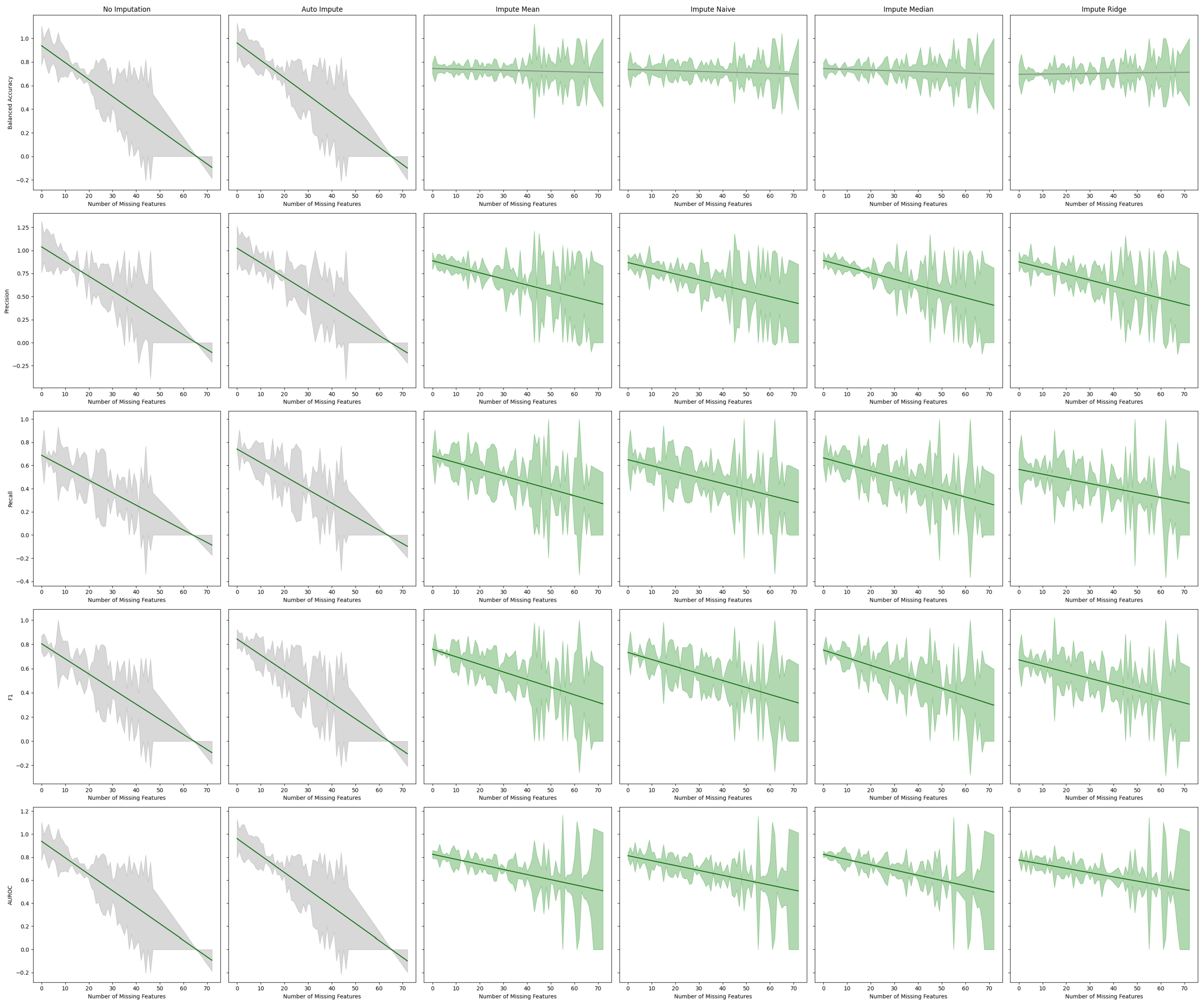
Figure 7.
Best fit lines of machine learning metrics as a function of the number of missing features. The shading is the residual of the best fit line. The best fit line is colored green if we reject the null hypothesis that the line has a slope of zero. The shading is colored green if we reject the null hypothesis that the residuals have constant variance.
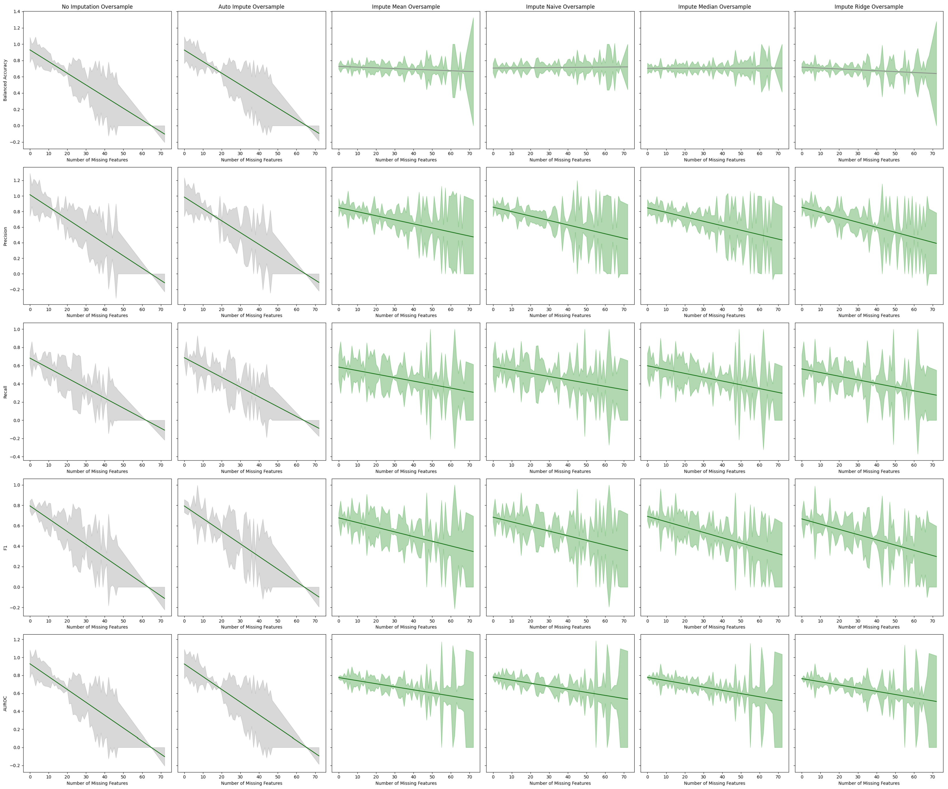
Figure 8.
Best fit lines of machine learning metrics as a function of the number of missing features. The shading is the residual of the best fit line. All models contain an oversampling step. The best fit line is colored green if we reject the null hypothesis that the line has a slope of zero. The shading is colored green if we reject the null hypothesis that the residuals have constant variance.
Table 1.
Model input features and missingness proportion for the total dataset for training and testing subsets.
| | Total | Training | Testing |
|---|
| Age | 0.000000 | 0.000000 | 0.000000 |
| Median income | 0.000000 | 0.000000 | 0.000000 |
| Deprivation index | 0.000000 | 0.000000 | 0.000000 |
| Chloride | 0.091448 | 0.091257 | 0.092210 |
| Bicarbonate | 0.653057 | 0.653368 | 0.651811 |
| Alanine aminotransferase | 0.144202 | 0.143750 | 0.146010 |
| Albumin | 0.138477 | 0.137825 | 0.141085 |
| Alkaline phosphatase | 0.140681 | 0.140218 | 0.142532 |
| Anion gap | 0.222889 | 0.222680 | 0.223723 |
| Aspartate aminotransferase | 0.145162 | 0.144927 | 0.146102 |
| Basophils | 0.155516 | 0.154991 | 0.157613 |
| Bilirubin | 0.159603 | 0.159277 | 0.160906 |
| Height | 0.006870 | 0.006940 | 0.006586 |
| Weight | 0.008790 | 0.008826 | 0.008649 |
| Calcium | 0.094230 | 0.093851 | 0.095750 |
| Carbon dioxide | 0.177928 | 0.177490 | 0.179681 |
| HDL | 0.331019 | 0.330497 | 0.333108 |
| LDL | 0.351579 | 0.350987 | 0.353944 |
| Creatinine | 0.083538 | 0.083301 | 0.084485 |
| Eosinophil | 0.151078 | 0.150606 | 0.152965 |
| Erythrocytes | 0.104615 | 0.104277 | 0.105968 |
| Heart rate | 0.008975 | 0.008941 | 0.009110 |
| Leukocyte | 0.089564 | 0.089203 | 0.091010 |
| Lymphocytes | 0.144079 | 0.143765 | 0.145333 |
| MCH | 0.139400 | 0.139079 | 0.140685 |
| MCHC | 0.140034 | 0.139695 | 0.141393 |
| MCV | 0.169126 | 0.168842 | 0.170263 |
| Monocytes | 0.146879 | 0.146420 | 0.148718 |
| Neutrophils | 0.143371 | 0.142896 | 0.145271 |
| Platelets | 0.115707 | 0.115226 | 0.117633 |
| Potassium | 0.103088 | 0.102984 | 0.103506 |
| Respiratory rate | 0.310053 | 0.308913 | 0.314610 |
| Sodium | 0.092913 | 0.092681 | 0.093841 |
| Triglyceride | 0.339421 | 0.339068 | 0.340833 |
| Urea nitrogen | 0.112839 | 0.112733 | 0.113262 |
| Vomiting | 0.000000 | 0.000000 | 0.000000 |
| Myocardial infarction | 0.000000 | 0.000000 | 0.000000 |
| Arthritis | 0.000000 | 0.000000 | 0.000000 |
| Polyuria | 0.000000 | 0.000000 | 0.000000 |
| Aspirin | 0.098970 | 0.098952 | 0.099043 |
| Beta blockers | 0.098970 | 0.098952 | 0.099043 |
| Steroids | 0.098970 | 0.098952 | 0.099043 |
| Acetaminophen | 0.098970 | 0.098952 | 0.099043 |
| Statin | 0.098970 | 0.098952 | 0.099043 |
| Opioids | 0.098970 | 0.098952 | 0.099043 |
| Nicotine | 0.098970 | 0.098952 | 0.099043 |
| Paraesthesia | 0.098970 | 0.098952 | 0.099043 |
Table 2.
Linear regression coefficients.
| Sensitive Attribute | Coefficient |
|---|
| Female | −0.54 |
| Male | 0.39 |
| Gender Other | 0.14 |
| Black | 1.31 |
| White | −1.34 |
| Middle Eastern | 0.48 |
| Asian | −0.09 |
| Race Other | −0.35 |
Table 3.
Tabular representation of
Figure 7. We display the Y-intercept and slope of the lines of best fit for the estimator performance on a given metric. The F-Test
p-value gives the probability of the null hypothesis that the line of best fit has a slope of zero. The Breusch–Pagan
p-value, which gives the probability that the error of the line has constant variance, is also given.
| Estimator | Metric | Y-Intercept | Slope | F-Test | Breusch–Pagan |
|---|
| p-Value | p-Value |
|---|
| No Imputation | Balanced Accuracy | 0.938288 | −0.014331 | 0.000000 | 0.372675 |
| Precision | 1.038484 | −0.015907 | 0.000000 | 0.683840 |
| Recall | 0.688205 | −0.010770 | 0.000000 | 0.380535 |
| F1 | 0.805173 | −0.012496 | 0.000000 | 0.934875 |
| AUROC | 0.938288 | −0.014331 | 0.000000 | 0.372675 |
| Auto Impute | Balanced Accuracy | 0.962040 | −0.014739 | 0.000000 | 0.352425 |
| Precision | 1.023924 | −0.015765 | 0.000000 | 0.681243 |
| Recall | 0.742006 | −0.011667 | 0.000000 | 0.657899 |
| F1 | 0.844082 | −0.013165 | 0.000000 | 0.760720 |
| AUROC | 0.962040 | −0.014739 | 0.000000 | 0.352425 |
| Impute Mean | Balanced Accuracy | 0.744528 | −0.000483 | 0.517161 | 0.000141 |
| Precision | 0.887014 | −0.006534 | 0.000078 | 0.000000 |
| Recall | 0.680919 | −0.005709 | 0.000068 | 0.001215 |
| F1 | 0.759957 | −0.006277 | 0.000007 | 0.000021 |
| AUROC | 0.825048 | −0.004409 | 0.000089 | 0.000099 |
| Impute Naive | Balanced Accuracy | 0.736591 | −0.000548 | 0.431844 | 0.000462 |
| Precision | 0.867793 | −0.006154 | 0.000095 | 0.000001 |
| Recall | 0.649528 | −0.005119 | 0.000186 | 0.005948 |
| F1 | 0.733024 | −0.005788 | 0.000016 | 0.000159 |
| AUROC | 0.812685 | −0.004257 | 0.000106 | 0.000334 |
| Impute Median | Balanced Accuracy | 0.743865 | −0.000620 | 0.384045 | 0.000024 |
| Precision | 0.890143 | −0.006735 | 0.000025 | 0.000000 |
| Recall | 0.665581 | −0.005631 | 0.000031 | 0.005150 |
| F1 | 0.752403 | −0.006318 | 0.000002 | 0.000065 |
| AUROC | 0.824385 | −0.004546 | 0.000030 | 0.000131 |
| Impute Ridge | Balanced Accuracy | 0.695296 | 0.000247 | 0.724879 | 0.000051 |
| Precision | 0.875240 | −0.006566 | 0.000036 | 0.000002 |
| Recall | 0.565600 | −0.004039 | 0.002779 | 0.007240 |
| F1 | 0.671835 | −0.005079 | 0.000164 | 0.000335 |
| AUROC | 0.775816 | −0.003679 | 0.000605 | 0.000196 |
Table 4.
Tabular representation of
Figure 8 displaying the Y-intercept and slope of the lines of best fit for the estimator performance with oversampling on a given metric. The F-Test
p-value, which gives the probability of the null hypothesis that the line of best fit has a slope of zero, is given. The Breusch–Pagan
p-value, which gives the probability that the error of the line has constant variance, is also given.
| Estimator | Metric | Y-Intercept | Slope | F-Test | Breusch–Pagan |
|---|
| p-Value | p-Value |
|---|
| No Imputation | Balanced Accuracy | 0.929096 | −0.014328 | 0.000000 | 0.485545 |
| Precision | 1.016151 | −0.015712 | 0.000000 | 0.913311 |
| Recall | 0.681390 | −0.010974 | 0.000000 | 0.125074 |
| F1 | 0.793971 | −0.012573 | 0.000000 | 0.761271 |
| AUROC | 0.929096 | −0.014328 | 0.000000 | 0.485545 |
| Auto Impute | Balanced Accuracy | 0.927235 | −0.014183 | 0.000000 | 0.510401 |
| Precision | 0.985620 | −0.015222 | 0.000000 | 0.935550 |
| Recall | 0.686184 | −0.010758 | 0.000000 | 0.247551 |
| F1 | 0.793458 | −0.012372 | 0.000000 | 0.783637 |
| AUROC | 0.927235 | −0.014183 | 0.000000 | 0.510401 |
| Impute Mean | Balanced Accuracy | 0.726784 | −0.000887 | 0.257000 | 0.003557 |
| Precision | 0.850450 | −0.005228 | 0.000794 | 0.000000 |
| Recall | 0.583068 | −0.003841 | 0.003761 | 0.017359 |
| F1 | 0.676989 | −0.004579 | 0.000297 | 0.000400 |
| AUROC | 0.775188 | −0.003411 | 0.001467 | 0.000415 |
| Impute Naive | Balanced Accuracy | 0.706228 | 0.000201 | 0.748666 | 0.000180 |
| Precision | 0.856446 | −0.005707 | 0.000332 | 0.000000 |
| Recall | 0.588463 | −0.003621 | 0.007300 | 0.003331 |
| F1 | 0.683514 | −0.004533 | 0.000638 | 0.000028 |
| AUROC | 0.780858 | −0.003407 | 0.001658 | 0.000215 |
| Impute Median | Balanced Accuracy | 0.702667 | 0.000042 | 0.943492 | 0.000159 |
| Precision | 0.846575 | −0.005729 | 0.000216 | 0.000000 |
| Recall | 0.597699 | −0.004181 | 0.001187 | 0.017877 |
| F1 | 0.691866 | −0.005232 | 0.000011 | 0.000528 |
| AUROC | 0.778030 | −0.003616 | 0.000513 | 0.000478 |
| Impute Ridge | Balanced Accuracy | 0.716799 | −0.001077 | 0.172684 | 0.003920 |
| Precision | 0.854813 | −0.006436 | 0.000026 | 0.000025 |
| Recall | 0.562891 | −0.004000 | 0.002777 | 0.017178 |
| F1 | 0.666654 | −0.005118 | 0.000037 | 0.000330 |
| AUROC | 0.763755 | −0.003537 | 0.000880 | 0.000269 |
| Disclaimer/Publisher’s Note: The statements, opinions and data contained in all publications are solely those of the individual author(s) and contributor(s) and not of MDPI and/or the editor(s). MDPI and/or the editor(s) disclaim responsibility for any injury to people or property resulting from any ideas, methods, instructions or products referred to in the content. |
© 2024 by the authors. Licensee MDPI, Basel, Switzerland. This article is an open access article distributed under the terms and conditions of the Creative Commons Attribution (CC BY) license (https://creativecommons.org/licenses/by/4.0/).


