A New Epidemic Model for the COVID-19 Pandemic: The θ-SI(R)D Model

Abstract

Since the beginning of the COVID-19 pandemic, a large number of epidemiological models have been developed. The principal objective of the present study is to provide a new six-compartment model for the COVID-19 pandemic, which takes into account both the possibility of re-infection and the differentiation between asymptomatic and symptomatic infected subjects. The model, denoted as θ-SI(R)D, is a six-compartment model, described by as many ordinary differential equations. The six compartments are denoted as Susceptible ($S$), Symptomatic Infected ($I_s$), Asymptomatic Infected ($I_a$), Recovered from Asymptomatic fraction ($R_a$), Recovered from Symptomatic fraction ($R_s$), and Deceased ($D$). Such a model has no analytical solutions, so we performed both a simulation and a model validation ($R^2=0.829)$. Based on the results of our simulations (and, on the other hand, on the results of most of the models in the scientific literature), it is possible to draw the reasonable conclusion that the epidemic tends, even without vaccination, to a steady state.

1. Introduction

Since the beginning of the COVID-19 pandemic, a large number of epidemiological models have been developed: for this purpose, a wide range of models was used (both stochastic and deterministic), some taken from the literature and others modified from the classic SIR (Susceptible, Infected, and Removed), SEIR (Susceptible, Exposed, Infected, and Removed), and SI(R) (also named SIRS: Susceptible, Infected, Removed, and Susceptible) models.

For example, Karako et al. [1] proposed a stochastic model applied to Japanese data.

Among the deterministic models, most of the authors used compartmental models based on the SEIR model: Kuniya [2] applied the classical model; Ahmad et al. [3] slightly adapted the classic SEIR model; Ivorra et al. [4] adopted a nine-compartment model (called SEIHRD); Li et al. [5] built a six-compartment model (called SEIRHD); Adhikari et al. [6] and Almeida at al. [7] started from a SEIR model in which they introduced a compartment Q for the quarantined (i.e., for the isolated subjects) and they called it SEIQR.

Each of these authors has contributed to a more precise understanding of the characteristics of the epidemic spread.

In fact, although it may be disappointing for some, the principal aim of a mathematical model is not, primarily, to enable forecasting, but rather to confirm the assumptions (specifically, in our case, the biological hypotheses) that are the basis of that model.

Regarding possible predictions, it must be clearly stated that, although possible, they would be valid only as long as the parameters of the model and the biological assumptions remain unchanged (i.e., under an unrealistic condition).

In May 2020, we proposed a SI(R) model [8] that, for the first time, included the hypothesis of not permanent immunity.

In that three-compartment model, we retrospectively separated both compartment I and compartment R into two sub-compartments corresponding to the asymptomatic and symptomatic subjects. Furthermore, we considered a closed population, with no births or deaths (considering these terms to be negligible in the short term). In this model, on the other hand, we separated the compartments of the symptomatic and asymptomatic infected and of the symptomatic and asymptomatic recovered patients; we also separated the compartment of the deceased due to COVID-19.

However, since that moment, other biological and epidemic information has become available. In detail, the vast proportion of asymptomatic subjects within the infected ones, has emerged, together with their primary relevance for the dissemination of SARS-CoV-2 [9].

Based on these considerations, the novelty of this study is chiefly its introduction, in addition to the already introduced hypothesis of not permanent immunity (a hypothesis, which turned out to be correct, that almost no other model has taken into consideration), of the separation between the compartments of the recovered and the deceased, as well as between asymptomatic and symptomatic subjects, to whom different parameters of recovery and lethality are attributed. Moreover, we considered an open population, introducing the terms of birth and mortality (but only for the Susceptible compartment, considering that these terms are negligible in the other compartments, apart from mortality from COVID-19, already considered).

This model also provides a certain amount of flexibility, for example, being able to easily differentiate both the force of the infection and the rate of loss of immunization between symptomatic and asymptomatic subjects.

2. Materials and Methods

The principal objective of the present study was to provide a new 6-compartment model for the COVID-19 pandemic, which takes into account both the possibility of re-infection and the differentiation between asymptomatic and symptomatic infected subjects.

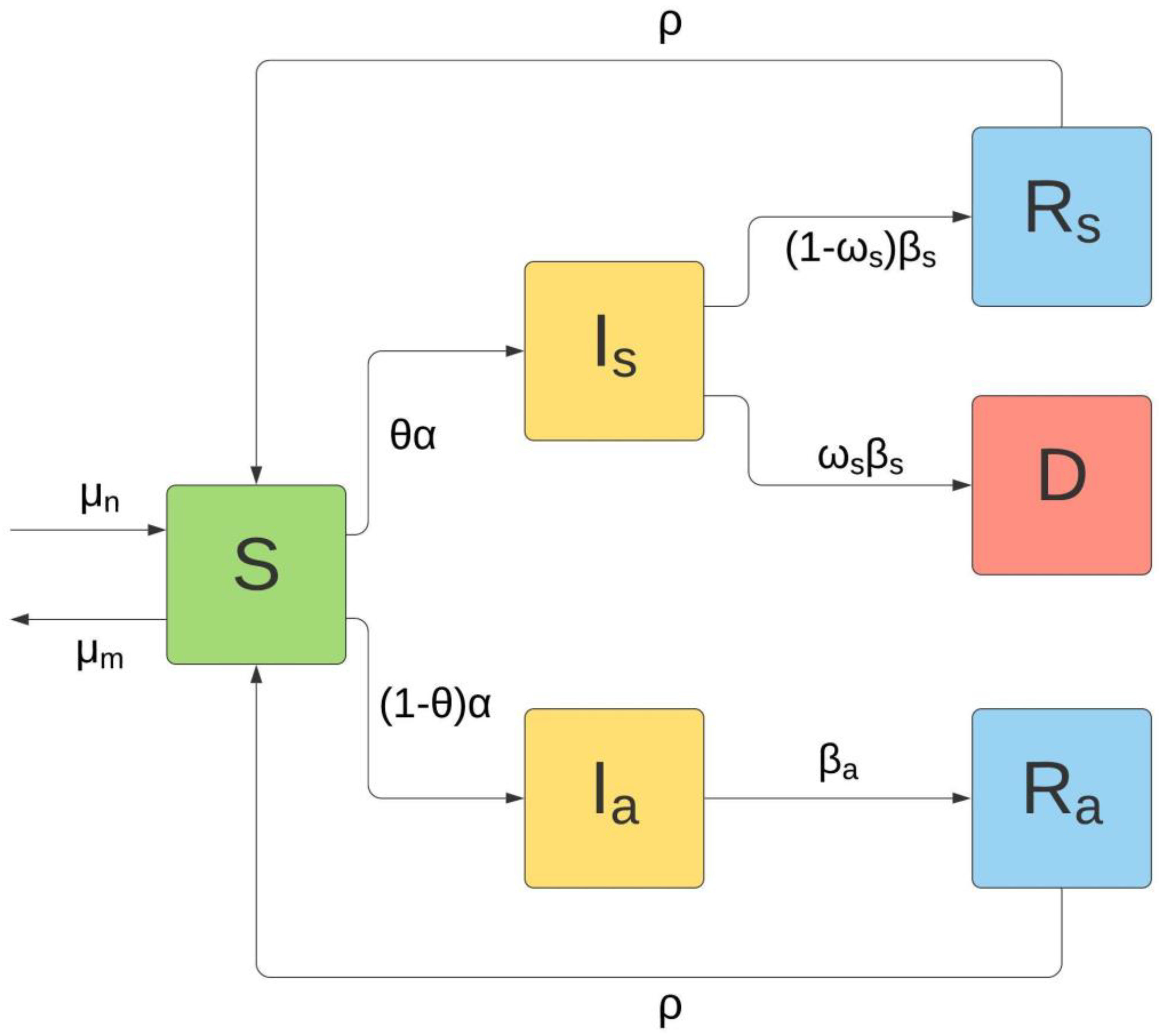
The model, denoted as θ-SI(R)D, is a 6-compartment model, described by as many ordinary differential equations. The six compartments are represented by Susceptible ($S$), Symptomatic Infected ($I_s$), Asymptomatic Infected ($I_a$), Recovered from Asymptomatic fraction ($R_a$), Recovered from Symptomatic fraction ($R_s$), and Deceased ($D$).

The biological assumptions are as follows:

• No entry or exit from the territory (closed territory);
• The contagiousness of the infected is immediate (therefore, the compartment of the Exposed of SEIR models is not considered);
• A loss of immunity is considered (in this version of the model, it is considered at a constant rate);
• Mortality and birth rate affect, as a first approximation, only the Susceptible compartment;
• The Asymptomatic Infected compartment includes both the fraction identified by laboratory diagnostic evaluation and the unidentified one;
• There is no lethality in the Asymptomatic Infected fraction.

The 6-compartment model is shown in Figure 1.

Mathematically, the model is described by the following system of six ordinary differential equations:

$$\{\begin{array}{c}\begin{array}{c}\frac{dS}{dt}={\mu }_{n}S-{\mu }_{m}S-\theta \alpha S{I}_s-\left(1-\theta \right)\alpha S{I}_a+\rho \left(R_a+R_s\right)\\ \frac{d{I}_a}{dt}=\left(1-\theta \right)\alpha S{I}_a-{\beta }_a{I}_a\\ \frac{d{I}_s}{dt}=\theta \alpha S{I}_s-{\beta }_s{I}_s\end{array}\\ \frac{d{R}_a}{dt}={\beta }_a{I}_a-\rho R_a\\ \frac{d{R}_s}{dt}=\left(1-{\omega }_s\right){\beta }_s{I}_s-\rho R_s\\ \frac{dD}{dt}={\omega }_s{\beta }_s{I}_s\end{array}$$

(1)

where $\alpha$ is the disease contact rate, also known as the force of infection; ${\beta }_a, {\beta }_s$ are the transition rates ($I_a$→$R_a$, and $I_s$→$R_s$, respectively); $\rho$ is the rate of loss of immunization; ${\omega }_s$ is the fatality rate in $I_s$ compartment; $\theta$ is the proportion of asymptomatic infected; ${\mu }_n$ is the natality rate; and ${\mu }_m$ is the mortality rate.

The first equation shows the variation over time of the compartment S; this subpopulation increases with the birth rate and with the loss of immunization of the recovered, while it decreases due to general mortality and contact with the infected (both symptomatic and asymptomatic) with a consequent transfer from S to $I_a$ and $I_s$.

The second and third equations show the variation over time of the compartments of the asymptomatic and symptomatic Infected $(I_a$ and $I_s),\mathrm{respectively}$. In both cases, the increase is due to the matching between Susceptible and Infected; the decrease, in the case of asymptomatic subjects, is due to the transition to the Recovered ($R_a$ compartment), while in the case of symptomatic subjects, it is due to the transition both to Recovered ($R_s$ compartment) and to Deceased (D compartment).

The fourth and fifth equations show the variation over time of the Recovered compartments of the asymptomatic and symptomatic fraction of the Infected. In both cases, the increase is due to the recovery or negativization of the Infected; the decrease is due to the return to the Susceptible compartment due to the loss of immunization.

The last equation shows the variation over time of the Deceased; the increase is due to the fraction of symptomatic Infected ($I_s$) that transitions to death (i.e., the fatality rate).

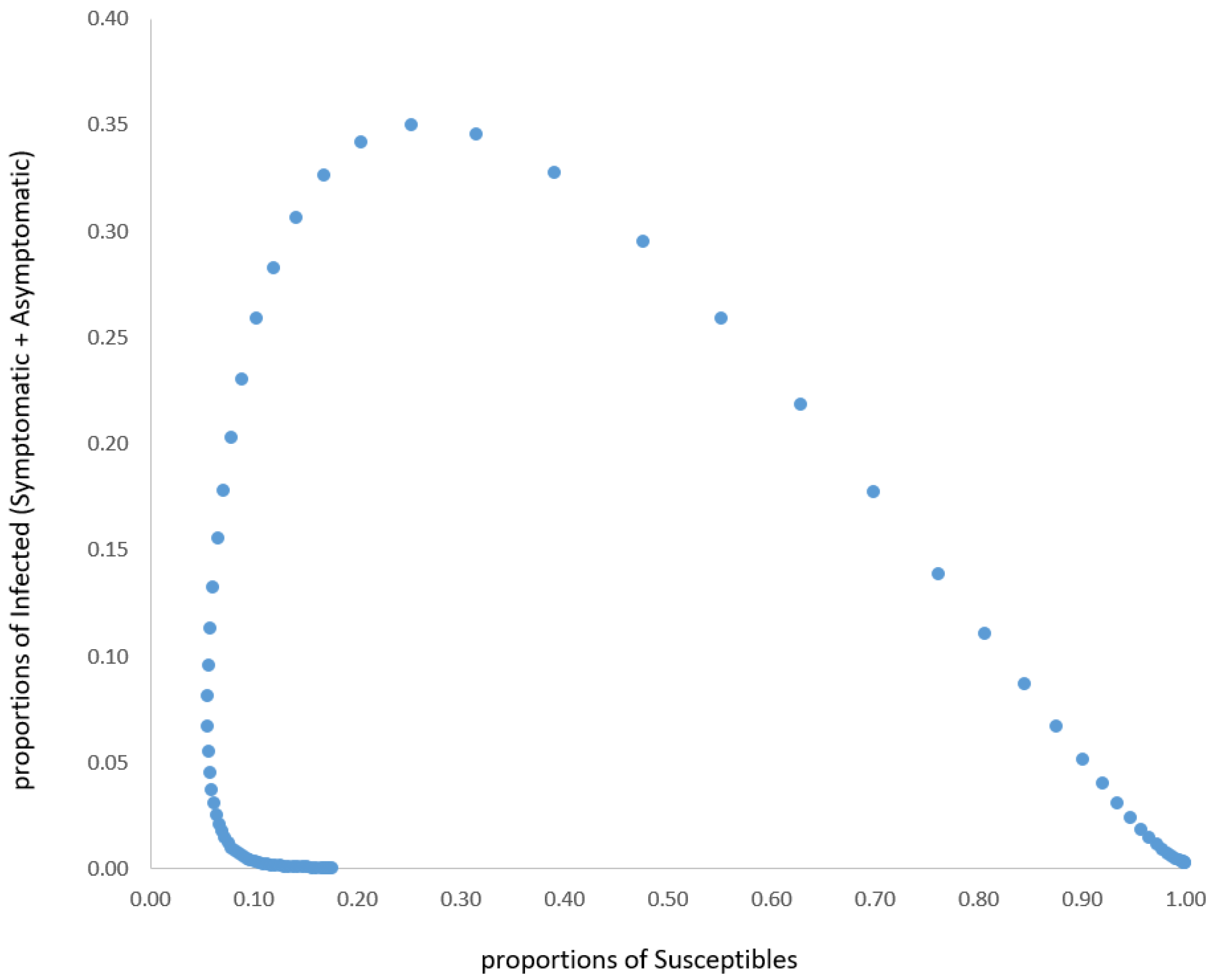
As such a model has no analytical solutions, we performed a simulation.

Concerning the parameters, we assumed (taking them from the biological literature and, especially, from pandemic official data [10,11]) the following values: α = 0.6; ${\beta }_a$ = 0.143; ${\beta }_s$ = 0.055; $\rho$ = 0.003; ${\mu }_n$ = 0.007; ${\mu }_m$ = 0.011; $\theta$ = 0.1; and ${\omega }_s$ = 0.14.

The simulation should be followed by a process of validation of the model, which is obtained with statistical methods allowing to evaluate the fitting of this model with the data observed from real life. Additionally, here there is a very important methodological problem: the data must be ’clean’. For example, this was not possible with the Italian data of COVID-19 for two reasons.

The first is that the data were largely incomplete, especially in the period of the so-called ‘first wave’: for example, all asymptomatic subjects were excluded, due to the health policies in force at that time. The second is that, at least in Italy, there has never been a serious sampling process for exclusively scientific purposes, although this was invoked by two former presidents of the ISTAT (the Italian National Institute of Statistics) with an open letter to the principal Italian newspaper [12]. Therefore, the data are affected by the fact that it has not been collected for the purpose of epidemiological investigation, but only for the purpose of contact tracing and isolation of potentially infected individuals.

In this situation, at least in Italy, Deceased data are theoretically the only “hard” variable in such a process of model validation, because the Italian official statistics do not discriminate between symptomatic and asymptomatic infected. Unfortunately, not even Deceased data is, in fact, a safe variable, since a re-adjustment of previous data happens very frequently. Furthermore, the issue of the distinction, never sufficiently defined, between Deceased “with COVID-19” and Deceased “caused by COVID-19” remains unsolved.

3. Results

Through the simulations, we can consider the numerical trends of the model that seems to converge towards a steady state, i.e., towards a state of equilibrium among the components of the population (Susceptible, Infected, and Recovered) (Figure 2 and Figure 3), but not towards a desirable extinction. This result is confirmed by the analysis of the trajectory in the phase space (Figure 4). Furthermore, it is important to underline that this model does not allow to find analytical solutions, so the results can only be referred to the set of parameters used to conduct the simulations.

However, in this situation of uncertainty, we tried to perform the model validation exclusively by fitting the Deceased data of Italy in the period of the so-called ‘first wave’ (from 24 February 2020 to 13 June 2020). We obtained an $R^2=0.829$, denoting an excellent fitting between the observed and expected Deceased.

Evidently, our model does not take into account, at the moment, the rising of virus variants, which seems to make a modification, at least, of the force of infection parameter necessary, and perhaps of the construction of further compartments as well, one for each variant.

Furthermore, in recent months, the impact of vaccination had to be considered, so the models had to be modified to take them into account (also in this case, we should probably have to consider different compartments, one for each kind of vaccine).

4. Conclusions

Based on the results of our simulations (and, on the other hand, on the results of most of the models in the scientific literature), it is possible to draw the reasonable conclusion that the epidemic naturally tends to a steady state, but not (and it is of extreme relevance) towards the extinction of the epidemic without a vaccination strategy. It is also reasonable to predict that the effect of vaccinations could lead either to a better steady state (i.e., with a steadily lower percentage of Infected and Deceased) or, hopefully, to the pandemic’s disappearance.

Regarding the points of weakness of this study, we wish to underline the following. (i) The model does not include different compartments for different virus strains; (ii) The model does not include the vaccination factor (in our opinion, this factor has to be differentiated, in the model, according to the different vaccine formulations); (iii) Due to data quality, it was not possible to evaluate the goodness of fit of real data for all the six compartments, but only for the Deceased one.

However, we consider our model to be a small, but significant, step towards a full comprehension of the SARS-CoV-2 pandemic. Evidently, other more complex models, built with other compartments and with a better estimation of the biological parameters, will greatly improve the pandemic understanding, which is the real purpose of a mathematical epidemic model.

It was essentially impossible to make a comparison with the other models proposed in the literature, due to the different sources of the data (and, above all, due to the low quality of the data), the different estimation of the parameters, and the different biological assumptions. In such a complex context, also the eventual confirmation of results obtained from another model would not represent an effective validation of our model. Even the comparison with our previous SI(R) model [8] is substantially impossible for the introduction of new compartments and new biological assumptions. However, in both cases, the achievement of a steady state is looming.

In fact, another lesson about mathematical models emerges from this pandemic: we must clarify that an epidemic model is a very simplified representation of reality, which takes into consideration only the relevant factors. Furthermore, it is primarily used to understand the phenomenon rather than to forecast it, as is also underlined by Panovska-Griffiths [13]. In a moment of excessive and clumsy scientific communication (often even by scientists, at least in Italy), it should be the starting point for any reflection based on epidemiological models.