Article

Improving Deep Segmentation of Abdominal Organs MRI by Post-Processing

Depto Engenharia Informática, Faculdade de Ciencias e Tecnologia, University of Coimbra, 3030-290 Coimbra, Portugal
BioMedInformatics 2021, 1(3), 88-105; https://doi.org/10.3390/biomedinformatics1030007
Submission received: 2 August 2021 / Revised: 13 October 2021 / Accepted: 14 October 2021 / Published: 19 October 2021

Abstract

:
Today Deep Learning (DL) is state-of-the-art in medical imaging segmentation tasks, including accurate localization of abdominal organs in MRI images. But segmentation still exhibits inaccuracies, which may be due to texture similarities, proximity or confusion between organs, morphology variations, acquisition conditions or other parameters. Examples include regions classified as the wrong organ, some noisy regions and inaccuracies near borders. To improve robustness, the DL output can be supplemented by more traditional image postprocessing operations that enforce simple semantic invariants. In this paper we define and apply totally automatic post-processing operations applying semantic invariants to correct segmentation mistakes. Organs are assigned relative spatial location restrictions (atlas fencing), 3D organ continuity requirements (envelop continuity), and smoothness constraints. A reclassification is done within organ envelopes to correct classification mistakes, and noise is removed (fencing, enveloping, noise removal, re-classifying and smoothing). Our experimental evaluation quantifies the improvement and compares the resulting quality with prior work on DL-based organ segmentation. Based on the experiments, we conclude post-processing improved the Jaccard index over independent test MRI sequences by a sum of 12 to 25 percentage points over the four segmented organs. This work has an important impact on research and practical application of DL because it describes how to post-process, quantifies the advantages, and can be applied to any DL approach.

1. Introduction

Magnetic Resonance Imaging (MRI) is an imaging technique based on capturing magnetic signal changes in the resonance of hydrogen protons after triggering radio-frequency pulses. Computerized processing of those signals outputs MRI images which can be used for diagnosing medical conditions. The resulting MRI scan is a sequence of slices, where a slice is a 2D image of the body part that is being scanned. A sequence of 2D images generates a clear 3D volume with details of the body part that was scanned. Deep learning-based segmentation networks can learn to segment automatically either the 2D slices or the 3D volumes based on training examples. They are state-of-the-art in segmentation of this and other medical imaging contexts.

1.1. Background on Segmentation of Abdominal Organs in MRI

The segmentation network is itself an evolution of the classification Convolution Neural Network (CNN). While the CNN is an image classifier that inputs an image and outputs a classification for the image, the segmentation network classifies each image pixel, resulting in a complete segmentation of the image. The segmentation network has an encoder, which is a sequence of convolution stages (convolution layers together with regularization and pooling) that extract and compress features automatically from the original image, and a decoder, which is a sequence of deconvolution layers, and a final pixel classification layer. The decoder effectively converts the compressed features back to an image sized segmentation map.
In this work, the targets of segmentation are a set of organs, in particular the liver, the spleen and the two kidneys. Figure 1 shows an example slice extracted from a full MRI abdomen sequence, with ground-truth segmentation shown on the left and segmentation results using CNN architecture named DeepLabV3 [1] on the right. It is possible to see some inaccuracies in the form of some wrongly classified pixels, most errors in the example being related to spilling to neighbor areas, and also a wrong classification of some areas as part of the organ.
In order to prepare the segmentation networks for segmentation, it was necessary to train them with a large number of training sequences and corresponding ground-truths (correct segmentations) for the networks to learn how to segment specific organs. We used the Chaos challenge data [2] as the dataset. The dataset includes 120 DICOM sequences from MRI. In total, there are 1064 slices, 80% used for training and the remaining for test (10%) and validation (10%). This dataset is further augmented to double the size using data augmentation (random translations of up to 10 pixels, random rotations up to 10 degrees, shearing up to 10 pixels and scaling up to 10%). The convolution network learns to segment based on the back-propagation algorithm, which iteratively adjusts convolution and deconvolution filter weights based on gradient descent methods to progress into minimization of the loss metric using a learning rate. The loss metric itself is a function that quantifies the segmentation error, a measure of the difference between the segmentation output and the ground-truth.

1.2. Contributions

Many factors can contribute to inaccuracies in the results of deep learning-based segmentation, and specifically of segmentation of abdominal organs. We already pointed out textures similarities, proximity or confusion between organs, morphology variations, acquisition conditions and other parameters as the major reasons for those errors, resulting in regions classified as the wrong organ, some noisy regions and inaccuracies near borders. Some simple examples of errors include classification of parts of a left kidney as a right kidney and vice-versa, erroneous classification of parts of the spleen as kidney or vice-versa, some other structures classified as one of the organs, some parts of the background classified as a part of an organ and spilling the organ segments into neighboring regions.
In all these examples a human can detect the errors, and the semantics that the human uses to detect the errors can be enforced automatically. Even a very good deep learning segmentation of abdominal organs might score between and 80% and 90% Jaccard index, leaving an additional 10 to 20% space for further improvement by post-processing. A solution for post-processing is to apply constraints based on the additional semantic invariants that are obvious to a human observer but not so obvious to the automated DL procedure. These invariants can, however, be coded as automated post-processing steps. One procedure reminiscent of atlas-based approaches is to obtain the expected 3D location and volume from the training images, with some tolerance added, whereby an organ is expected to be located in a specific region of the body and to have a certain volume (we call this procedure “fencing”). Additionally, this fencing also allows us to remove incorrect assignments and to do reclassification of regions inside the incorrect fence. Another constraint is continuity, whereby the segment of an organ is expected to have continuity inside of its 3D and 2D structures, and to form a solid organ envelope. This allows the algorithm to fill gaps and also connect parts of disconnected regions within an organ’s envelope. Additionally, small, isolated regions outside the 3D envelope can be considered noise and reclassified. Finally, smoothness is expected. Under smoothness, borders of organ volumes and slices should be smooth. In essence, the proposed approach applies a set of image processing operations using several techniques to improve segmentation.
In this work, we first propose the post-processing operations, then we build an experimental setup to quantify the quality improvement. For the experimental setup we first compare the quality of segmentation of three well-known off-the-shelf segmentation networks to choose the best performing one. Before engaging in experimental work, we first tuned training parameters by evaluating the quality of segmentation, as measured by the metric IoU (intersect-over-the-union) on the test set as we varied learning rates (0.01, 0.005, 0.001, 0.0005, 0.0001), different learning algorithms (Adaptive Moment estimation = Adam, Root Mean Square Propagation, and RMSProp, Stochastic Gradient Descent with Momentum = SGDM), different numbers of epochs (70, 100, 300, 500,700), different minibatch numbers (8, 16, 32, 64) and momentum (1, 0.9). The top performing alternative was chosen (0.005 learning rate, SGDM, 500 epochs, 32 minibatch size, momentum 0.9) and used for the experimental runs. After choosing and tuning the network, it was trained with MRI sequences and then used to segment an independent set of test MRI sequences. Finally, we applied the post-processing operations to improve the results and assess the amount of improvement. Our assessment was based on evaluating the quality of segmentation of the liver, spleen, left kidney and right kidney, and the quality after post-processing, to understand how much the post-processing operations were able to improve the quality of the result. Using this experimentation approach, we were able to conclude that post-processing operations improved the Jaccard index of segmentation by 12 to 25 percentage points for total improvement over the four organs in our experimental setup. We also reviewed the quality achieved by related works segmenting abdominal organs, for comparison purposes. Finally, we showed how post-processing transformed a real test sequence. We conclude that the approach improves the robustness of segmentation by correcting errors, an important advantage being that it can be applied to improve the quality of the outputs of any segmentation network.

2. Related Work

Precise segmentation of abdominal organs is a relevant task for several clinical procedures, including visual aids to diagnosis, detailed analysis of abdominal organs for correct positioning of a graft prior, abdominal aortic surgery and many other tasks. Ongoing research tries to improve segmentation results and to overcome many challenges due to the highly flexible anatomical properties of the abdomen and limitations of modalities reflected in image characteristics. Previously, segmentation would be done mostly using multi-atlas techniques, with interesting results when applied to different anatomical parts. For instance, Bereciartua et al. [3] segmented the liver using a 3D liver model guided by a precomputed probability map. Le et al. [4] used histogram-based liver segmentation with a subsequent geodesic active contour refinement step, and Huynh et al. [5] used watershed transformation and active contours. In many of these approaches, organ volumes and statistical information regarding those volumes were often used as part of the segmentation process. In the last few years, deep learning-based approaches have been quickly overtaking traditional ones in the task of segmentation of medical images in general and for MRI segmentation of abdominal organs specifically.
Deep learning approaches not only improve segmentation scores significantly when compared to more traditional techniques, they are also much more capable of learning and adapting automatically. However, many of the image processing concepts used in prior approaches are still relevant in the deep learning era. In the next paragraphs we review previous deep learning approaches applied to segmentation of abdominal organs in both MRI and CT sequences.
Zhou et al. [6] showed that fully convolutional networks (FCN) produce excellent results in segmentation of abdominal organs from computer tomography (CT) scans. Zhou et al. [6] transformed the anatomical structure segmentation on 3D CT volumes into a majority voting of the results of 2D image segmentation on a number of 2D-slices from different image orientations, then an organ localization module was used with two major processing steps: (1) individual organ localization that decides the bounding box of a target organ based on window sliding and pattern matching in Haar-like and LBP feature spaces; (2) group-wise calibration and correction based on general Hough voting of multiple organ locations. Bobo et al. [7] applied the approach to segmentation of the whole abdomen from magnetic resonance imaging sequences (MRI). The authors show that fully convolutional neural networks (FCN) improve abdominal organ segmentation significantly when compared with multi-atlas methods. The FCN they used resulted in a dice similarity coefficient (DSC) of 0.930 for the spleen, 0.730 for the left kidney, 0.780 for the right kidney, 0.913 for the liver and 0.56 for the stomach. Larsson et al. [8] proposed SeepSeg, a method to segment abdominal organs based on three steps: (1) localization of region of interest using a multi-atlas approach; (2) pixelwise binary classification using a convolutional neural network and (3) post-processing by thresholding and removing all positive samples except the largest connected component. In this approach, the authors found a region of interest for each organ, which was done as a pre-processing step for a classification network to classify fewer voxels. The authors achieved IoU (Intersect-over the Union, a.k.a Jaccard coefficient) scores of 0.90, 0.87, 0.76 and 0.84, respectively, for liver, spleen, right and left kidneys. Groza et al. [9] proposed an ensemble of networks and voting for output in the segmentation of MRI scans. There were five different networks used for the final averaged ensemble. The first was the DualTail-Net architecture, which consisted of an encoder part and two independent decoder parts. The other four networks had very similar U-Net-based architectures, and the final result was an averaged ensemble of predictions obtained by the five networks. Conze et al. [10] also worked in the segmentation of MRI scans. They tested several segmentation network architectures, including a deeper version of UNet using VGG19 instead of VGG16, comparing one version training from scratch to one starting from pretrained nonmedical data. The authors also cascaded two networks, combining two v19pUNet networks by inputting posterior probabilities resulting from the first v19pUNet output into the second one. In another alternative, the cascaded pipeline was used as generator within a conditional Generative Adversarial Network (cGAN), a model including a discriminator whose role was to distinguish real ground-truth segmentations from those arising from the generator, to strengthen the ability of the generative part to create segmentation masks that are as realistic as possible. From the various architectures tested by Conze, the most significant improvements came from UNet with VGG19, and also to a smaller degree by the two cascaded UNets. In [11] the authors proposed a convolutional neural network (CNN)-based fully automated MR image-based multi-organ segmentation technique, namely ALAMO (Automated deep Learning-based Abdominal Multi-Organ segmentation). A multi-slice 2D neural network was developed to account for information between adjacent slices. Within the study, the authors investigated multiple approaches, including network normalization, data augmentation, and deeply supervised learning. They also introduced a novel multiview training and inference technique. As part of the work the authors compared two popular networks, PlainUnet and DenseUnet, showing that DenseUnet used fewer parameters and offered more accurate segmentation results. By adding multiple skip connections within the convolutional blocks, the network was forced to reuse its weights, thus dramatically reducing the number of parameters for the same performance. The authors also showed that normalization had insignificant performance gain and combining three different views could boost performance further.
These approaches reviewed focused mostly on architectural variations, multiple views, ensembles and voting to try to improve the quality of segmentation. Not as much focus has been placed on the central idea we explore in this work, which is that relevant improvement can also be obtained by applying post-processing operations that enforce semantic invariants. The use of post-processing operations to improve the quality of segmentation also has the advantage of robustness, since whatever network architecture is chosen, the quality of the resulting images and segmentation depends on acquisition details, morphology and other factors. Details such as low contrast between the tissue near the borders of organs and surrounding tissue, calibration specifics, morphology variations along slices and between different patients, and multiple other factors, can result in better or worse segmentation quality, even when top performing architectures are used. In that context, and to improve the chances of a best-possible result regardless of the network architecture, a set of post-processing steps that apply relevant semantic concepts is a very useful add-on to make the results robust to variability. In this paper we define, apply and experiment with post-processing operations that can correct and improve the final quality of segmentation of the abdominal organs, thus complementing previous works on segmentation of MRI sequences of abdominal organs.

3. The Post-Processing Approach

In this section we define a sequence of post-processing operations to be applied automatically to the output of segmentation of an MRI sequence scanning the abdominal organs. The segmentation convolution neural network outputs a segmentation which is then passed through the following set of operations: (1) organs are first assigned relative 3D spatial location restrictions (fencing), based on the locations in training data; (2) a re-classification is done within organs envelops to correct classification mistakes and remove wrong classifications; (3) in-organ holes filling and 3D organ continuity filling are applied (enveloping), and finally surface smoothness operations are used to smooth the surface.
The ground-truth MRI sequences are an essential element in the post-processing operations, since the expected volumes of the organs (an atlas or each organ) are obtained automatically from those sequences. Each slice is an image-sized labelmap (ground-truth labelmap), i.e., each pixel contains the pixel class label. The labels identify the structure or organ that the pixel belongs to, labeling 0 for background (no class). The output of segmentation is also a labelmap, which we denote as “segmentation labelmap”. The purpose of post-processing is to transform the segmentation labelmaps using invariants inferred from the ground-truth labelmaps. We also define the term organmap as being a labelmap containing only one of the organs, which is obtained from a labelmap by zeroing all labels except the one identifying the specific organ to keep (the organmap can also be transformed into a binary map by assigning 1 to the organ label).
Besides the labelmaps, we generate a (contiguous) regionsmap for the 3D volume. While labelmaps label pixels based on the class they belong to, the regionsmap labels pixels based on the labels based on pixels connectivity in the image. This allows us to distinguish different connected regions of each organ in the segmentation output and enables further automatic reasoning regarding those regions.
The operations we describe next are, in order: “fencing”, “class re-assignments and removal of noise”, “computation and filling of organs envelops” and “slice smoothing and filling”.

3.1. Fencing (Expected Location Constraint)

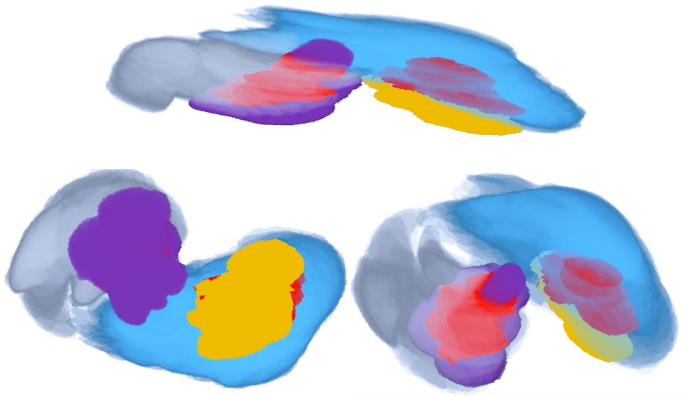
Conceptually, the fence is a 3D volume that defines maximum organ size and/or positions for each organ. The fence is defined for each organ separately. Given the set of training sequences, the fence of one organ is the union of all 3D volumes of that organ in the training sequences. A dilation operation follows [12] (imdilate function in matlab) to add a volume tolerance (δ) over the union of volumes (δ-dilation over the union of organ volumes V; we used δ = 5 pixels).
In order to compute the fence given the MRI training set, the ground-truth sequences are first aligned in the scan sequence dimension using image registration algorithm [13]. The second step involves, for each organ O present in the ground-truth sequences, isolation of O in all sequences and computation of the union of all volumes of O in all sequences, resulting in a volume V that contains all volumes of the instances of that organ in all training sequences.
Algorithm 1 shows the steps involved in pseudo-code. In that code, the loop of step 2 cycles over each organ. In that loop, for each organ, we create an initial empty 3D volume with the size of the largest sequence (step 2a), then for each sequence (step 2.b) we OR its 3D volume with the current organ volume (sout{end}) (step 2.b.i). After processing all training sequences we simply apply an imdilate function [12] (step 2.d).
Algorithm 1: 3D FencingComments
Input: training ground-truth sequences s as 3D array s{},
organ ids in ground-truth idx[]
Output: 3D fence for each organ fence{organ}[]
1. fence={};
2. for i = 1:length(idx)                  % for each organ
   a. fence{end+1}=zeros(maxX, maxY, maxZ);      % create fence space
   b. for i = 1:length(s)                % for each sequence
       i. fence{end}=fence{end} OR s{i}(idx organ) % OR the sequence
   c. end
   d. fence{end}=imdilate(fence{end}, δ);        % add δ-dilation
3. end
Considering the abdominal organs liver, spleen and kidneys, Figure 2 illustrates three different views of the union of organ volumes obtained from the training ground-truths. Blue stands for the liver, yellow and purple stand for kidneys and grey stands for the spleen. The red volumes show intersections of two or more organs, i.e., a spatial volume where more than one organ can appear in the union of all training sequences.

3.2. Class Reassignments and Removal of Noise

After fencing, class reassignments and noise removal are done using a set of steps.
  • Define the largest continuous spatial region of a specific organ, O, as the main volume of that organ.
  • For each region that is classified as another organ, O′, but is completely within the organ fence and which has a volume larger that a predefined threshold (the threshold was set to 500 pixels in our experiments), consider it as organ O (reclassify).
  • For each region that is classified as another organ O’ but is completely within the organ fence and which has a volume smaller than the predefined threshold (the threshold was set to 500 pixels in our experiments), consider it as background (reclassify to background).
  • Regions classified as organ O, but which are smaller than a certain threshold (i.e., “too small regions”) are considered noise and reclassified as background (the threshold was set to 500 pixels in our experiments).
Regarding implementation details, Algorithm 2 shows the main steps involved. The inputs to the algorithm are the segmentation outputs, denoted as 3D arrays in a set of sequences s{[]} and the fences. In that algorithm step 2 processes each sequence separately, and step 2.b iteratively obtains the volumes of pixel classifications as each organ, so that the algorithm can process each organ separately from the segmentation output. Next the fence is applied to zero all pixels outside the fence (step 2.b.ii), keeping only organ pixels that are inside of it. The next step (steps 2.b.iii and 2.b.iv) identifies the largest region as being the specific organ being processed in the current iteration. To do that, an organ regions labelmap (bw) is created from the organ volume using bwlabel [14] (step 2.b.iii). The sizes of regions are next calculated on those bw regionmaps (number of occurrences of each label). The region label with top number of occurrences identifies the largest region, and therefore the organ extent (step 2.b.iv). Finally, step 2.b.v reclassifies regions classified as other organs inside the organ fence and having sizes larger than a threshold (500 pixels) as being part of the organ itself. Since those regions are inside the fence of the organ and are not small, they are wrongly classified as another organ and should, therefore, be reclassified. The remaining regions with volume lower than 500 are reclassified as background (step 2.b.vi). Step 2.b.vii removes regions that were classified as the organ but are actually disconnected from its main volume (have a different label in the bw labelmap) and have sizes lower than a threshold (500 pixels).
Given the imperfections of segmentation near borders (including spurious pixel classifications as part of the region and sometimes thin connections to neighbour regions), we also found out that the best results were obtained by preceding the calculation of the largest region by morphological erosion [15] then calculating and isolating the largest region, subsequently applying dilation [15] with the same structuring element and size to reverse the previous erosion operation. The erosion frequently eliminates noise in the borders and some spurious connections to neighbouring regions.
Algorithm 2: Class re-assignments and removal of noiseComments
Input: segmentation outputs as sets of 3D arrays, each being one sequence s{sequence[]},
organ ids in ground-truth idx[], fences fence{organ}
Output: cleaned segmentation outputs s{sequence[]}
1. sout={};
2. for i = 1: length(s)                       % for each sequence
   a. sout{end+1}=zeroed 3D sequence volume;
   b. for j = i:length(idx)                  % for each organ
      i. O = zeroed 3D organ sequence volume;
      ii. volO=s{i} & fence{idx}            % organ’s fence
      iii. bw=bwlabel(volO)=>regions         % label differently each connected region
      iv. O = bw(bw=max(countEachLabel(bw)))  % max volume region within fence
      v. bw(idx2:volO~=idx && countLabel(bw, idx2)>500)=idx=>volO  % reclassify to organ
      vi. bw(idx2:volO~=idx && countLabel(bw, idx2)<=500)=idx=>volO  % reclassify to bkgnd
      vii. bw(idx2:volO==idx && countLabel(bw, idx2)<=500)=background=>volO %remove noise
      viii. sout{end}= sout{end}|volO         % add the organ volume to the sequence
   c. end
3. end

3.3. Computation and Filling of Organ Envelopes

After filling each slice individually (imfill [12]), the next step joins disconnected regions that are inside the organ’s fence and are classified as the same organ. In this context, a discontinuity is a gap between two regions of an organ in the sequence of MRI slices. The space between the disconnected regions is filled by interpolation between the border pixels of the two extremity slices bordering the gap. Figure 3 illustrates the objective. In the figure, the space between the two regions r1 and r2 is filled by interpolation.
The result after all the previous operations is a 3D envelope of each organ based on the largest volume classified as that organ, and the remaining major volumes reclassified as that organ within the fencing volume of the organ, with the space between the parts filled to create a solid.

3.4. Slice Smoothing and Filling

Slices smoothing is the process of improving each slice by removing small protruding pixels, filling holes and smoothing edges of each organ independently. The steps are shown in Algorithm 3. For this algorithm, slices are processed in sequence. For each organ in each slice, the first part of the algorithm (steps 1.a.i to 1.a.iii) removes small protruding pixels from the main volume. This is done using a 2D erode operator (imerode [12]) to isolate the main volume from spurious pixels, keeping only the largest region, and then applying a dilate operator (imdilate [12]) to restore the organ area to the original size. Step 1.a.iv fills holes inside the organ region using the imfill morphological operator ([12,16]). The final step 1.a.v smooths contours. This works on the binary image of the organ in the slice. The step first blurs the contours using a 3 × 3 2-D average pixel value convolution. From the output of the blurring, all pixels with value smaller than 0.5 are zeroed. The resulting nonzero pixels are the extent of the smoothed organ.
Algorithm 3: Slice smoothing and fillingComments
Input: sequence of 2D slices s[]
Output: sequence of cleaned 2D slices s[]
1. For each slice si in s
   a. for each organ sio isolated from si
      i. apply 2D erode operator imerode [12] to sio (uses a structuring elem with size as parameter, we used square and size 3 empirically)
      ii. Keep the largest region by applying labeling of connected regions and counting the number of pixels of each region:
        1. bw=bwlabel(sio)=>regions  %label differently each connected region
        2. R = bw(bw=max(countEachLabel(bw))) %max region in slice
        3. Delete all but R
      iii. Apply a 2D dilate operator imdilate [12] to sio (structuring elem as well, we used square and size 3 empirically)
      iv. Fill holes inside sio using imfill morphological operator ([12,16])
      v. Smooth contours of sio by blurring and re-thresholding (blur using 2-D average convolution, then keep intensities >0.5)
   b. End
   c. Reconstruct si from the modified sio for all organs as the union of all sio
2. end

3.5. Illustrating Result of Post-Processing Transformations

Figure 4 is an illustration of transformation based on the above-described operations (fencing-enveloping-noise removal-reassignment-smoothing). It shows what happened when a specific test image was segmented using the DeepLabV3, followed by the post-processing operations that corrected the output. In the figure, the liver is orange, the kidneys are yellow and purple, and the spleen is green. Figure 4a shows the ground-truth abdominal organs. Figure 4b shows the segmentation output, where some errors can be seen (e.g., part of the spleen was classified as right kidney, another part as left kidney and only a smaller region is correctly classified as spleen; the right kidney region is infiltrated by a region with a few contiguous slices classified wrongly as liver; there are also some small noisy regions, including some larger noise outside fences, e.g., on top of the spleen). Figure 4c shows the final corrected result after applying all the post-processing transformations. Fencing removed some of the imperfections, such as the incorrect regions classifications as right kidney in the left part of the figure. Enveloping and reclassification transformed those and other incorrect regions standing inside the fence of spleen into spleen and merged the resulting parts. It also transformed the region inside the right kidney that was incorrectly classified as liver into right kidney, and finally smoothing smoothed the slices to obtain the final result shown in Figure 4c. Although still not exactly equal to the original model, the post-processed Figure 4c is much closer to the original Figure 4a than the segmented Figure 4b.

4. Materials and Methods

In this section we first describe the architecture of the segmentation networks used in our experiments, then we describe the dataset and details of the experimental setup.

4.1. Segmentation Networks

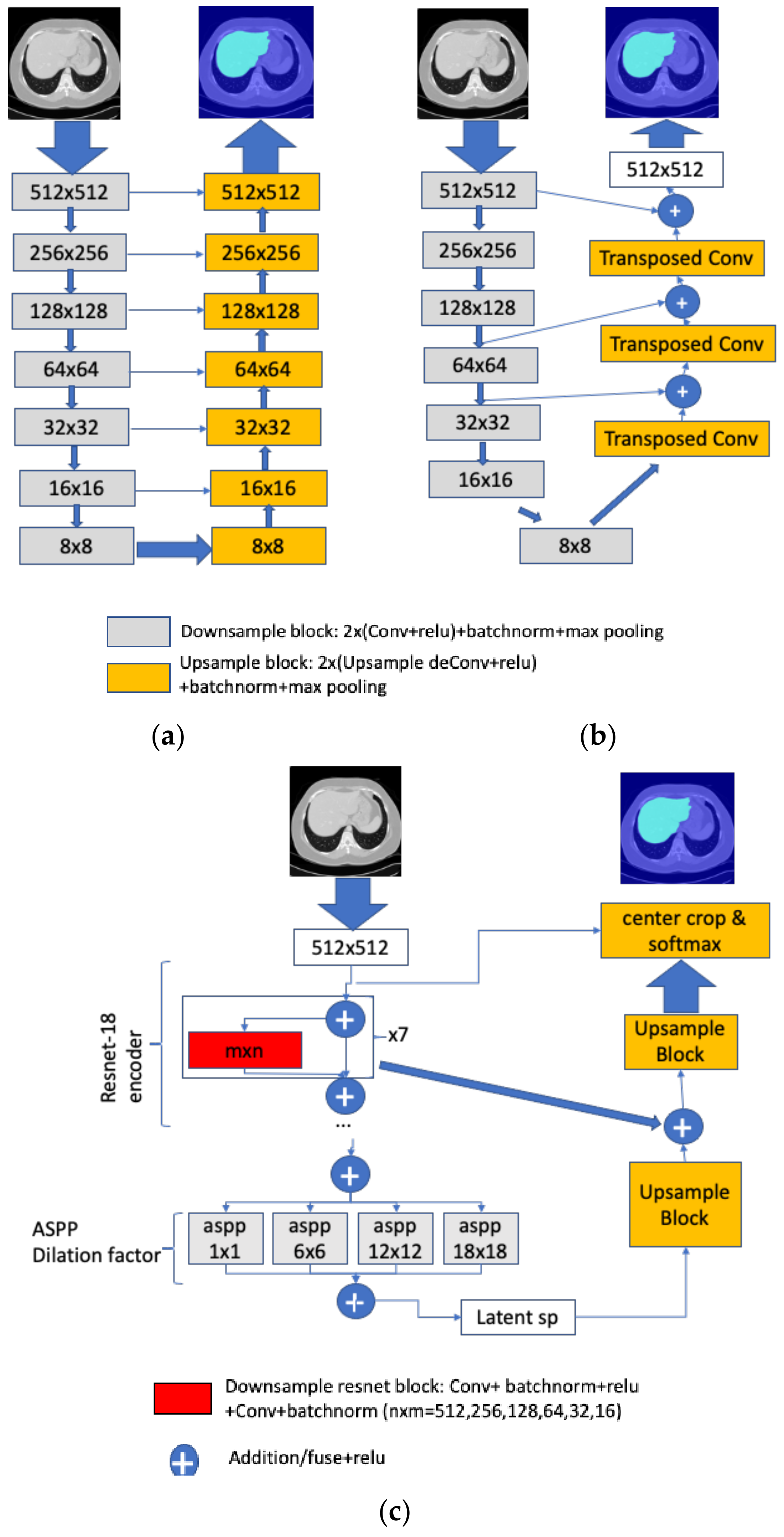
The architecture of the segmentation network is a relevant factor for the quality of segmentation; therefore, a lot of prior research has focused on improving architectures. In this work we follow the strategy of choosing a best-performing network from a set of popular architectures widely used in medical imaging in general. The U-Net [17], DeepLabv3 [1] and FCN [18] are our choices of networks, and our focus is on the following sequence: (1) first compare those base networks with the dataset used for the experiments, including data augmentation and other training optimizations to pick the best-performing architecture for the experimental setup used; (2) try to maximize the quality by testing training options, in particular this led us to experiment with a successful modification of the loss function; (3) experiment with the post-processing functionality using that network. Next, we describe the base network architectures used.
U-Net. U-Net is a 58-layer segmentation network using VGG-16 stages for feature extraction (encoding), followed by an intermediate section connecting encoder to decoder, and a decoding section that is symmetric to the encoding section. Figure 5a summarizes the layers of U-Net. The encoding section consists of contraction blocks applying two 3 × 3 convolution layers followed by a 2 × 2 max pooling layer. The decoding section is symmetric to the encoding section, consisting of the same number of expansion blocks as there are contraction blocks in the encoding section. As with encoding, each expansion block has two 3 × 3 convolution layers followed by a 2 × 2 up-sampling layer. But each expansion block also appends feature maps from the corresponding contraction block. The rationale is that features learnt in the contracting block of the image will be used to reconstruct it at the symmetric stage.
FCN. The structure of FCN is sketched in Figure 5b. FCN also uses VGG-16 (with seven stages, corresponding to 41 layers) as encoder, plus a much smaller sequence of up-sampling layers (decoding stages) for a total network size of 51 layers. FCN also forwards feature maps (the pooled output of coding stage 4 is fused with output of the first up-sampling layer, and the pooled output of coding stage 3 is fused with the output of the second up-sampling layer). Finally, the image input is also fused with the output of the third up-sampling layer, all this followed by the final pixel classification layer.
DeepLabV3. DeepLabV3 is the deepest network tested in this work, with 100 layers and a generic layout of layers shown in Figure 5c. DeepLabV3 uses Resnet-18 as feature extractor, with eight stages totaling 71 layers, the remaining stages being Atrous Spatial Pyramid Pooling (ASPP), plus the final stages. Forwarding connections are also added from encoding stages to the ASPP layers for enhanced segmentation of objects at multiple scales. The outputs of the final DCNN layer are combined with a fully connected Conditional Random Field (CRF) for improved localization of object boundaries using mechanisms from probabilistic graphical models.

4.2. Dataset

The magnetic resonance imaging data used in our experimentation is CHAOS Dataset, a publicly available set of scans in [2]. Table 1 lists the main dataset configurations. The data consists of 120 MRI sequences capturing abdominal organs (liver, kidneys and spleen) obtained using the T1-DUAL fat suppression protocol. Table 1 summarizes the dataset configurations. The sequences were acquired by a 1.5T Philips MRI, which produces 12-bit DICOM images with a resolution of 256 × 256. The ISDs varies between 5.5–9 mm (average 7.84 mm), x-y spacing is between 1.36–1.89 mm (average 1.61 mm) and the number of slices is between 26 and 50 (average 36). In total there are 1594 slices (532 slice per sequence) used for training and testing, with the testing sequences being chosen randomly to include 20% of all sequences in 5-fold cross-validation runs. Given the relatively limited size of the dataset, data augmentation was added after we verified that it would contribute to improved scores by increasing diversity and the size of the dataset.

4.3. Training and Sequence of Experiments

Data augmentation was defined based on random translations of up to 10 pixels, random rotations up to 10 degrees, shearing up to 10 pixels and scaling up to 10%. The networks were pretrained on object recognition tasks (Imagenet dataset). Network training was configured using SGDM as the learning algorithm, with an initial learning rate = 0.005 and piecewise learning rate with a drop period of 20 and a learn rate drop factor of 0.9 (the learn rate would decrease to 90% every 20 epochs). The default loss function used was cross-entropy (crossE), but we also experimented with post-processing on the segmentation output of the network trained with IoU loss. We include IoU loss because we found out that it improved the quality of segmentation of individual organs. Class balancing was applied in the pixel classification layer, training iterations were 500 epochs after we verified that convergence to a stable loss is achieved before that with minibatch size = 32, and momentum = 0.9. The training and testing were done on a machine with a GPU NVIDEA G Force GTX1070. The experiments were divided into two phases. The first phase involved choosing the best performing segmentation network. Using the chosen network we then proceeded to segment all MRI test sequences and then applied automatic post-processing to all sequences. The last step involved evaluating the quality of the results. We focused our analysis using global metrics and per-class IoU (a.k.a. Jaccard index JI), since this is a reliable and common metric for evaluation of segmentation performance.

4.4. Development Environment and Libraries Used

The coding for this work was done on Matlab R2019b and required the image processing toolbox, the deep learning toolbox, the computer vision toolbox and the deep learning toolbox model for the Resnet-18 network. The DeepLabv3 segmentation network was built using the deeplabv3plusLayers function. The FCN architecture was built using the fcnLayers function and the UNet used function unetLayers. The networks were trained using the trainNetworks function with training options defined using the trainingOptions object. The MRI images were handled by imageDatastore objects, and the ground-truths were handled by pixelLabelDataStore objects. The code for post-processing was all written from scratch in Matlab using multidimensional arrays to keep the training and test data and Matlab library functions to implement the necessary image processing operations. Matlab functions used as helpers to implement the steps included bwlabel, imbinarize, bwareafilt, morphological operations such as imfill, imerode, imdilate, and convolution operations using conv2. Links for code Supplementary Materials are given in the end of the work.

5. Experimental Results and Interpretation

In this section we evaluate the proposed post-processing approach. Our experiments were based on first choosing the best-performing network, then presenting the post-processing results in the form of evaluation of the amount of improvement derived from applying it. Finally, we review performance results from related works on both MRI and CT of abdominal organs to put our results in perspective in relation to the performances reported in those works.

5.1. Choosing the Best-Performing Network

Table 2 shows the results of the first part of our experiments, finding the best-performing base network. As described in the experimental setup, these results were obtained with data augmentation. IoU (JI) and Dice of the three segmentation network architectures is reported. The best-performing network was deepLabV3 (2 percentage points (pp) better than FCN, FCN being 3 pp better than UNET). For that reason, we proceeded with the next experiments using deepLabV3.

5.2. Post-Processing Results

For the next experiment we took the segmented sequences after applying deeplabV3-based segmentation to the original test sequences and ran them through the sequence of post-processing operations. The experiment was divided into two main tests to reflect the use of two different loss functions, i.e., cross entropy (crossE, the default loss function) and IoU. We included the two loss functions because IoU loss improved the quality of segmentation further. That way, we were able to compare the amount of improvement with the base crossE loss to that with already improved segmentation scores using IoU.
Table 3, Table 4, Table 5 and Table 6 show our results concerning the effects measured as IoU and Dice of applying the post-processing improvements in sequence. Table 3 and Table 4 report the results using IoU as the loss function, and Table 5 and Table 6 shows the results using crossE, the default loss function. Each column in the tables identifies the organ and the last column is the sum of percentage points (pp) increase in IoU or Dice over all organs. The first row shows the IoU/Dice of the base segmentation results, then each other row shows the IoU/Dice achieved after each post-processing operation.
The results in the tables essentially show that the post-processing steps were quite useful. Fencing improved the quality of segmentation by 2 pp in Table 3 (IoU loss) and by 8 pp in Table 5 (crossE loss). The next operation, re-classification and noise reduction, had the most significant contribution in both cases (6 pp and 9 pp for IoU and crossE loss respectively), and the final operation (enveloping, filling and slice filling and smoothing) contributed with 5 and 8 pp increases, respectively. The contributions were larger in the experiment with crossE because the base segmentation had more errors in that case. In general, these results prove that post-processing improved the results significantly. Importantly, we applied post-processing in a specific experiment setting and with a specific dataset and network, but it can be generalized to any approach and dataset since the defined post-processing steps are not dependent on either the network, the experimental settings or datasets tested.

5.3. Brief Comparison with Related Approaches

In this section we first compare the final scores obtained after post-processing in our experimental work with some techniques based on the architectural features tested on the same dataset. Then, we review some of the best scores obtained for segmentation of abdominal organs by other authors using a variety of techniques that include improved network architectures and ensembles, many of those works segmented CT scans, others segmented MRI scans. We converted scores to IoU (Jaccard index) when necessary, since many of those works report scores using the dice metric.
Table 7 compares several architectural variations from the work [10] that include the U-Net, a modified U-Net with VGG-19 instead of VGG-16 (V19UNet), a pretrained version (V19pUNet) and finally a cascade of two V19pUNet (V19pUnet1-1). The results show that our post-processing approach is better than any of these.
Table 8 shows the quality of segmentation achieved by related MRI (first three cases) and CT segmentation approaches as reported by the authors in their own papers. As can be seen from the table, there are many related approaches, and the reported scores vary significantly and also depend on the dataset used. From Table 8, refs. [19,20] achieve high scores in MRI segmentation of some of the organs (only the liver in [20]). Hu et al. [21,22] obtained the best results for CT, usually above 90%. The scores we obtained after post-processing (Table 3 and Table 5) are higher than [7] and comparable to some of the best scores reported in related works segmenting MRI sequences (e.g., [19]). Most importantly, the scores on those advanced architectures would also benefit from applying our post-processing approach, since it can be applied to any segmentation technique.

6. Post-Processing Extended Example

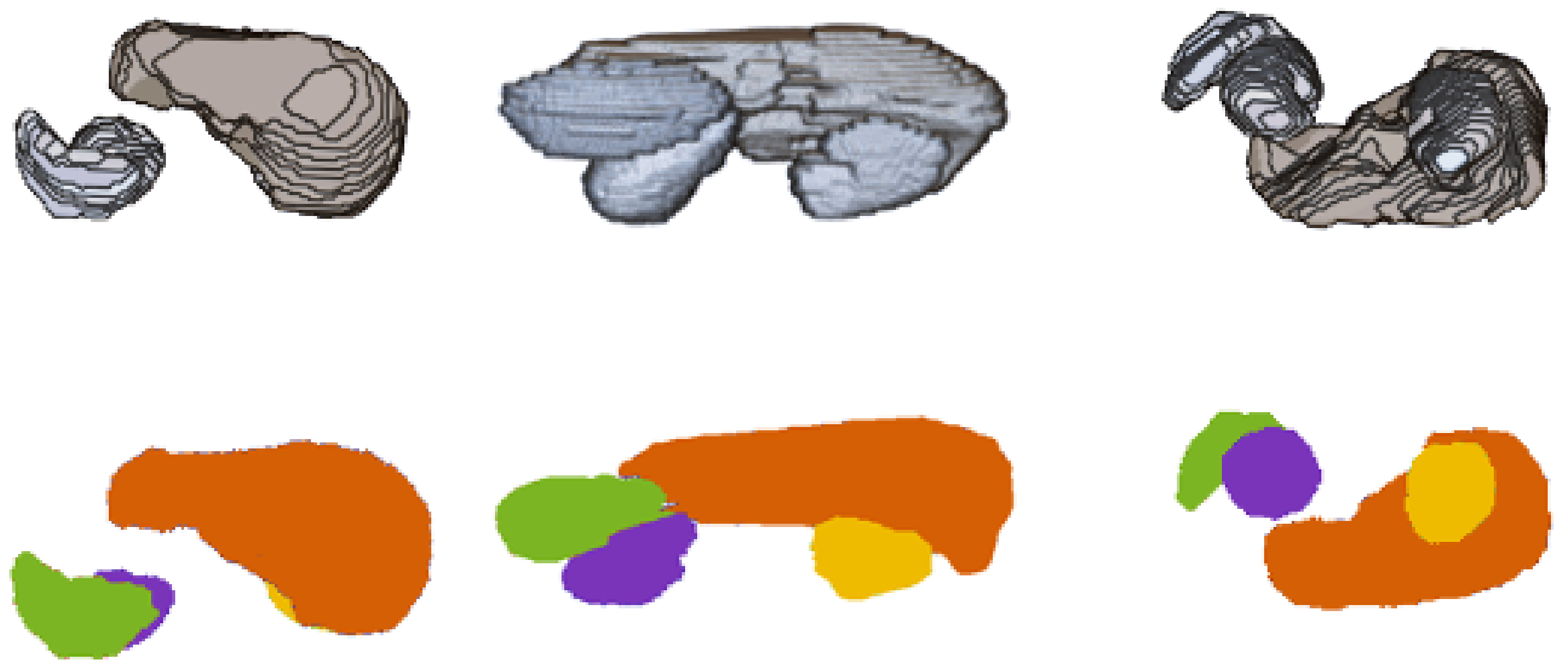
Figure 6 shows a 3D depiction of the sequence of slices of abdominal organs from a real test sequence. The 3D depiction is shown as a 3D model that includes all four organs (liver, spleen, right and left kidney), and also as a 3D coloured regions model (spleen is green, liver is orange, right kidney is yellow and left kidney is purple).
Figure 7 shows the output of segmentation using DeepLabV3 with the default cross entropy loss function. Once again, we show the 3D model plus the 3D coloured regions. We can see from both models, and especially from the 3D coloured model, that there are several inaccuracies in the output, including regions classified incorrectly as another organ.
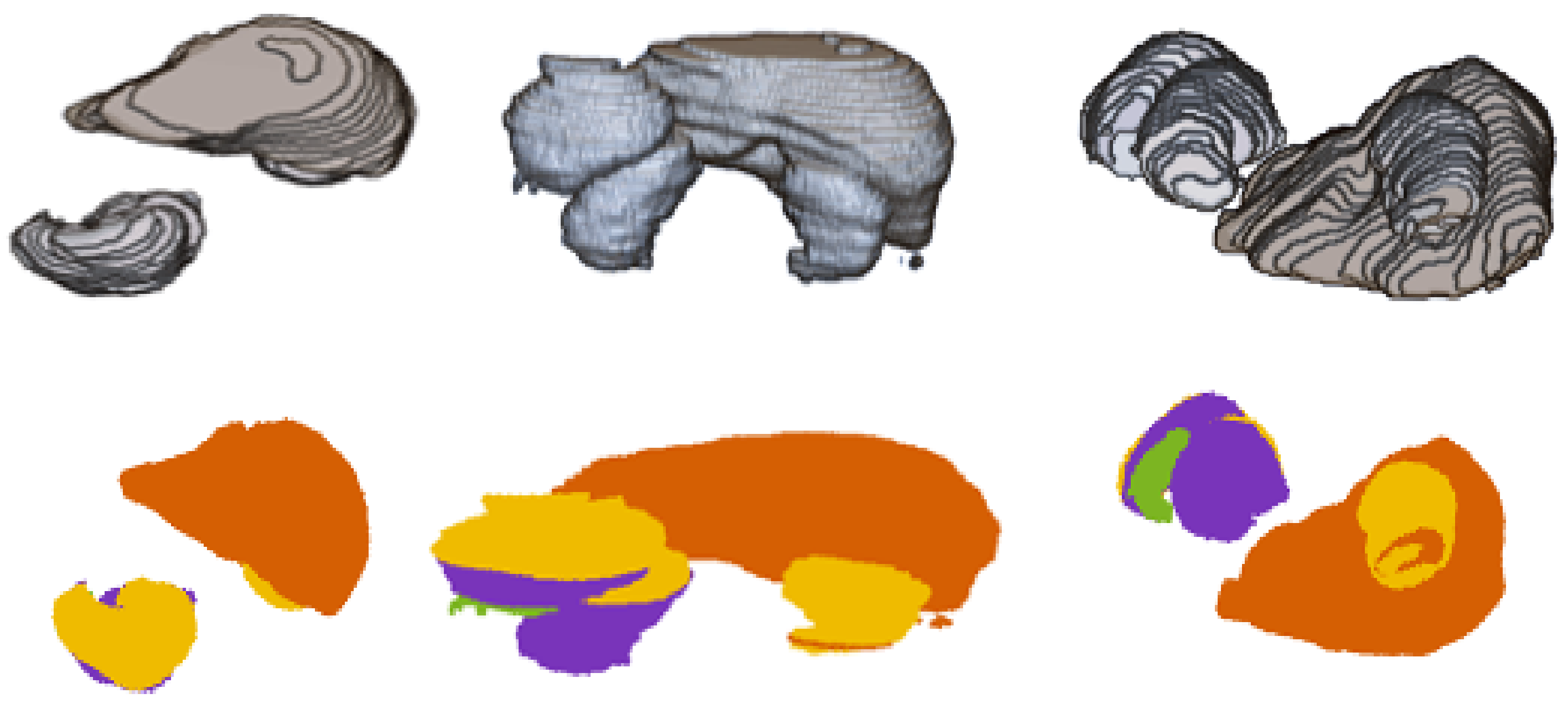
Figure 8 shows the 3D coloured model of the results after post-processing. We can see that incorrect region classifications were corrected, especially in the spleen and left kidney regions, and in the right kidney region as well. Some noise was also removed.

7. Conclusions and Future Work

Deep learning-based segmentation is an established procedure for segmentation of MRI and CT sequences. In spite of the amazing quality of the results, there are still imperfections, and researchers search for approaches to improve the quality of the results. Many works have explored advances in segmentation network architectures and the use of ensembles and voting. We propose and evaluate a complementary approach of image post-processing for enforcement of semantic invariants (fencing, enveloping, noise removal, reassignment and smoothing) to improve the results. The approach is defined in detail, and in the experimental section we tested the degree of improvement achieved from the post-processing steps. We used a publicly available dataset to show that the approach improved segmentation scores by a sum of 12 to 25 percentage points over the four organs tested.
Our focus in this work has been on improving the quality of segmentation output by means of post-processing, which can be applied regardless of the architecture of the segmentation CNN. Our future work on this issue will explore two major improvements. On one hand, we intend to find an approach to integrate post-processing into the network architecture itself as additional layers. The advantage will be to integrate this post-processing in the back-propagation learning procedure. On the other hand, we also wish to investigate several relevant evolutions to current state-of-the-art segmentation using deep learning. Concerning the use of U-Net for segmentation of MRI, those relevant innovations include Attention Gates (AGs) [26], Squeeze-and-Excitation (SE) blocks [27] and Squeeze-and-excitation networks [28], which improve generalization performance in multicentric studies. Our future work also involves testing the approach with CT scans and together with advanced techniques that include ensembles of networks with voting.

Supplementary Materials

The following are available online: https://github.com/pedronunofurtado/postprocess, base code functions used in this work for testing postprocessing; https://github.com/pedronunofurtado/codingLOSS, code used for testing networks with loss functions.

Funding

This research received no external funding.

Institutional Review Board Statement

Not applicable.

Informed Consent Statement

Not applicable.

Data Availability Statement

The dataset used is public and all relevant details are provided. Additional information is provided on demand.

Acknowledgments

We used a publicly available MRI dataset for our experiments. The dataset can be found in [2,29,30]. We acknowledge the organizers for allowing researchers to use these data.

Conflicts of Interest

The authors declare no conflict of interest.

References

  1. Chen, L.; Papandreou, G.; Kokkinos, I.; Murphy, K.; Yuille, A. Deeplab: Semantic image segmentation with deep convolutional nets, atrous convolution, and fully connected crfs. IEEE Trans. Pattern Anal. Mach. Intell. 2017, 40, 834–848. [Google Scholar] [CrossRef] [PubMed]
  2. Kavur, A.; Sinem, N.; Barıs, M.; Conze, P.; Groza, V.; Pham, D.; Chatterjee, S.; Ernst, P.; Ozkan, S.; Baydar, B.; et al. CHAOS Challenge—Combined (CT-MR) Healthy Abdominal Organ Segmentation. arXiv 2020, arXiv:2001.06535. [Google Scholar]
  3. Bereciartua, A.; Picon, A.; Galdran, A.; Iriondo, P. Automatic 3D model-based method for liver segmentation in MRI based on active contours and total variation minimization. Biomed. Signal Process. Control 2015, 20, 71–77. [Google Scholar] [CrossRef]
  4. Le, T.-N.; Bao, P.T.; Huynh, H.T. Fully automatic scheme for measuring liver volume in 3D MR images. Bio-Med. Mater. Eng. 2015, 26, S1361–S1369. [Google Scholar] [CrossRef] [PubMed] [Green Version]
  5. Huynh, H.T.; Le, T.-N.; Bao, P.T.; Oto, A.; Suzuki, K. Fully automated MR liver volumetry using watershed segmentation coupled with active contouring. Int. J. Comput. Assist. Radiol. Surg. 2016, 12, 235–243. [Google Scholar] [CrossRef] [PubMed]
  6. Zhou, X.; Takayama, R.; Wang, S.; Zhou, X.; Hara, T.; Fujita, H. Automated segmentation of 3D anatomical structures on CT images by using a deep convolutional network based on end-to-end learning approach. In Medical Imaging 2017: Image Processing; International Society for Optics and Photonics: Bellingham, WA, USA, 2017; Volume 10133, p. 1013324. [Google Scholar] [CrossRef]
  7. Bobo, M.; Bao, S.; Huo, Y.; Yao, Y.; Virostko, J.; Plassard, A.; Landman, B. Fully convolutional neural networks improve abdominal organ segmentation. In Medical Imaging 2018: Image Processing; International Society for Optics and Photonics: Bellingham, WA, USA, 2018; Volume 10574, p. 105742V. [Google Scholar]
  8. Larsson, M.; Zhang, Y.; Kahl, F. Robust abdominal organ segmentation using regional convolutional neural networks. Appl. Soft Comput. 2018, 70, 465–471. [Google Scholar] [CrossRef] [Green Version]
  9. Groza, V.; Brosch, T.; Eschweiler, D.; Schulz, H.; Renisch, S.; Nickisch, H. Comparison of deep learning-based techniques for organ segmentation in abdominal CT images. In Proceedings of the 1st Conference on Medical Imaging with Deep Learning (MIDL 2018), Amsterdam, The Netherlands, 4–6 July 2018. [Google Scholar]
  10. Conze, P.; Kavur, A.; Gall, E.; Gezer, N.; Meur, Y.; Selver, M.; Rousseau, F. Abdominal multi-organ segmentation with cascaded convolutional and adversarial deep networks. arXiv 2020, arXiv:2001.09521. [Google Scholar]
  11. Chen, Y.; Ruan, D.; Xiao, J.; Wang, L.; Sun, B.; Saouaf, R.; Yang, W.; Li, D.; Fan, Z. Fully Automated Multi-Organ Segmentation in Abdominal Magnetic Resonance Imaging with Deep Neural Networks. arXiv 2019, arXiv:1912.11000. [Google Scholar]
  12. Gonzalez, R.C.; Woods, R.E.; Eddins, S.L. Digital Image Processing Using MATLAB; Gatesmark Publishing: Knoxville, TN, USA, 2009. [Google Scholar]
  13. Viergever, M.; Maintz, J.; Klein, S.; Murphy, K.; Staring, M.; Pluim, J. A Survey of Medical Image Registration—Under Review. Med. Image Anal. 2016, 33, 140–144. [Google Scholar] [CrossRef] [PubMed] [Green Version]
  14. Haralick, R.; Shapiro, L. Computer and Robot Vision; Addison-Wesley: Boston, MA, USA, 1992; Volume I, pp. 28–48. [Google Scholar]
  15. Boomgard, V.; van Balen, R. Methods for Fast Morphological Image Transforms Using Bitmapped Images. CVGIP Graph. Models Image Process. 1992, 54, 254–258. [Google Scholar]
  16. Soille, P. Morphological Image Analysis: Principles and Applications; Springer: Berlin/Heidelberg, Germany, 1999; pp. 173–174. [Google Scholar]
  17. Ronneberger, O.; Fischer, P.; Brox, T. U-net: Convolutional networks for biomedical image segmentation. In Proceedings of the International Conference on Medical Image Computing and Computer-Assisted Intervention, Munich, Germany, 5–9 October 2015; Springer: Cham, Switzerland, 2015; pp. 234–241. [Google Scholar]
  18. Long, J.; Shelhamer, E.; Darrell, T. Fully convolutional networks for semantic segmentation. In Proceedings of the IEEE Conference on Computer Vision and Pattern Recognition, Boston, MA, USA, 7–12 June 2015; pp. 3431–3440. [Google Scholar] [CrossRef] [Green Version]
  19. Fu, Y.; Mazur, T.R.; Wu, X.; Liu, S.; Chang, X.; Lu, Y.; Li, H.H.; Kim, H.; Roach, M.; Henke, L.; et al. A novel MRI segmentation method using CNN-based correction network for MRI-guided adaptive radiotherapy. Med. Phys. 2018, 45, 5129–5137. [Google Scholar] [CrossRef] [PubMed]
  20. Chlebus, G.; Meine, H.; Thoduka, S.; Abolmaali, N.; Van Ginneken, B.; Hahn, H.K.; Schenk, A. Reducing inter-observer varia-bility and interaction time of MR liver volumetry by combining automatic CNN-based liver segmentation and manual corrections. PLoS ONE 2019, 14, e0217228. [Google Scholar] [CrossRef] [PubMed]
  21. Hu, P.; Wu, F.; Peng, J.; Bao, Y.; Chen, F.; Kong, D. Automatic abdominal multi-organ segmentation using deep convolutional neural network and time-implicit level sets. Int. J. Comp. Assist. Radiol. Surg. 2016, 12, 399–411. [Google Scholar] [CrossRef] [PubMed]
  22. Wang, Y.; Zhou, Y.; Shen, W.; Park, S.; Fishman, E.; Yuille, A. Abdominal multi-organ segmentation with organ-attention networks and statistical fusion. Med. Image Anal. 2019, 55, 88–102. [Google Scholar] [CrossRef] [PubMed] [Green Version]
  23. Kim, J.; Lee, J.-G. Deep-learning-based fast and fully automated segmentation on abdominal multiple organs from CT. In Proceedings of the International Forum on Medical Imaging in Asia, Singapore, 7–9 January 2019; SPIE: Bellingham, WA, USA, 2019; Volume 11050, p. 110500K. [Google Scholar]
  24. Gibson, E.; Giganti, F.; Hu, Y.; Bonmati, E.; Bandula, S.; Gurusamy, K.; Davidson, B.R.; Pereira, S.P.; Clarkson, M.J.; Barratt, D.C. Towards Image-Guided Pancreas and Biliary Endoscopy: Automatic Multi-organ Segmentation on Abdominal CT with Dense Dilated Networks. In Proceedings of the Medical Image Computing and Computer Assisted Intervention—MICCAI 2017, Quebec City, QC, Canada, 11–13 September 2017; pp. 728–736. [Google Scholar]
  25. Roth, R.; Shen, C.; Oda, H.; Sugino, T.; Oda, M.; Hayashi, H.; Misawa, K.; Mori, K. A multi-scale pyramid of 3D fully convo-lutional networks for abdominal multi-organ segmentation. In Proceedings of the International Conference on Medical Image Computing and Computer-Assisted Intervention, Granada, Spain, 16–20 September 2018; pp. 417–425. [Google Scholar]
  26. Schlemper, J.; Oktay, O.; Schaap, M.; Heinrich, M.; Kainz, B.; Glocker, B.; Rueckert, D. Attention gated networks: Learning to leverage salient regions in medical images. Med. Image Anal. 2019, 53, 197–207. [Google Scholar] [CrossRef] [PubMed]
  27. Rundo, L.; Han, C.; Nagano, Y.; Zhang, J.; Hataya, R.; Militello, C.; Tangherloni, A.; Nobile, M.S.; Ferretti, C.; Besozzi, D.; et al. USE-Net: Incorporating Squeeze-and-Excitation blocks into U-Net for prostate zonal segmentation of multi-institutional MRI datasets. Neurocomputing 2019, 365, 31–43. [Google Scholar] [CrossRef] [Green Version]
  28. Hu, J.; Shen, L.; Albanie, S.; Sun, G.; Wu, E. Squeeze-and-Excitation Networks. IEEE Trans. Pattern Anal. Mach. Intell. 2020, 42, 2011–2023. [Google Scholar] [CrossRef] [PubMed] [Green Version]
  29. Kavur, A.E.; Gezer, N.S.; Barış, M.; Aslan, S.; Conze, P.-H.; Groza, V.; Pham, D.D.; Chatterjee, S.; Ernst, P.; Özkan, S.; et al. CHAOS Challenge—Combined (CT-MR) Healthy Abdominal Organ Segmentation. Med. Image Anal. 2021, 69, 101950. [Google Scholar] [CrossRef] [PubMed]
  30. Kavur, A.E.; Gezer, N.S.; Barış, M.; Şahin, Y.; Özkan, S.; Baydar, B.; Yüksel, U.; Kılıkçıer, Ç.; Olut, Ş.; Akar, G.B.; et al. Comparison of semi-automatic and deep learning-based automatic methods for liver segmentation in living liver transplant donors. Diagn. Interv. Radiol. 2020, 26, 11–21. [Google Scholar] [CrossRef] [PubMed]
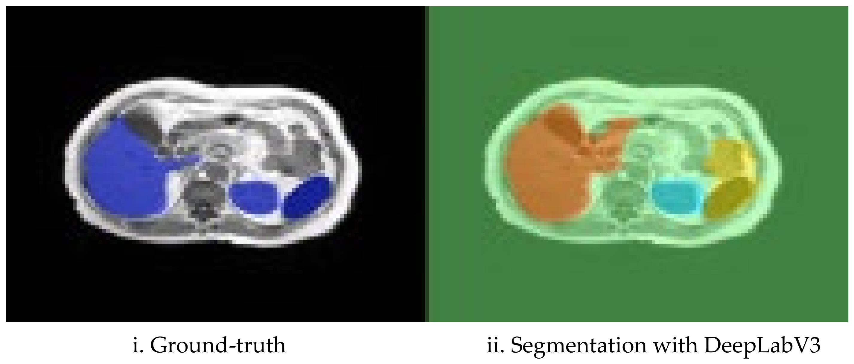
Figure 1. Example MRI sequence segmentation. The ground-truth in the left shows the organ extents of the liver, kidney and spleen that are exposed in this specific slide (blue means organ). On the right we show the corresponding pixel classifications by the segmentation network, where the colours are coded as: light blue = kidney, gold = spleen, red = liver. It is possible to see that the liver segment spills well off the organ, a region above the spleen is classified as spleen and, finally, the borders of all three organs are overcome by the segments.
Biomedinformatics 01 00007 g001
Figure 2. Illustration of semitransparent dilated union of organ volumes. The figure shows the union of locations of organs in 3D, taken from the training dataset in our experiments. The union is shown from three perspectives, which are front, bottom and top. In the figure, the liver in blue, the two kidneys are gold and purple, respectively, and the spleen is grey. Regions shared by more than one organ are red. The fence is obtained using a dilation (imdilate operator [12]) of each individual organ.
Biomedinformatics 01 00007 g002
Figure 3. Illustration of space filling. Given a main volume of an organ (region r1) and another smaller region (region r2) classified as the same organ inside its fence, the algorithm interpolates between each pixel of the extremity of r2 and r1. (a) Two regions, same organ. (b) Illustration of space filling operation. (c) Resulting organ.
Biomedinformatics 01 00007 g003
Figure 4. Illustrating before and after transformations. (a) Original. (b) Segmented. (c) Post-processed.
Biomedinformatics 01 00007 g004
Figure 5. Architectures of segmentation networks used. (a) U-Net segmentation network. (b) FCN segmentation network. (c) DeepLabV3 segmentation network.
Biomedinformatics 01 00007 g005
Figure 6. Original test sequence with organs as 3D and coloured 3D models.
Biomedinformatics 01 00007 g006
Figure 7. Segmented test sequence with organs as 3D and coloured 3D models.
Biomedinformatics 01 00007 g007
Figure 8. Post-processed segmented organs.
Biomedinformatics 01 00007 g008
Table 1. Summary of dataset configuration.
ParameterValue
Machine1.5T Philips MRI
Acquisition protocolT1-DUAL fat suppression
Image resolution12-bit DICOM images, resolution 256 × 256
ISDs5.5–9 mm (average 7.84 mm)
x-y spacing1.36–1.89 mm (average 1.61 mm)
Number of sequences120
Number of slices1594
Number of slices per sequence26 to 50 (average 36)
Test data20% sequences, 5-fold cross-validation runs
Table 2. IoU of segmentation networks with base crossE loss.
IoUDice
ClassDeepLabV3FCNUNETDeepLabV3FCNUNET
Background99%99%98%99.5%99.5%99%
Liver86%86%74%93%93%85%
Spleen82%74%73%90%85%84%
rKidney77%78%75%87%87.6%86%
lKidney81%77%78%89.5%87%87.6%
Avg IoU85%83%80%92%91%89%
Table 3. Improvement (metric = IoU) when IoU used as loss function.
StepLiver
(IoU)
Spleen
(IoU)
R Kidney
(IoU)
L Kidney
(IoU)
Pp Increase
(Sum)
Base segmentation0.860.870.860.84-
Fencing0.860.870.870.852
Re-assignments and noise redux0.880.890.870.876
Enveloping, filling and slice filling and smoothing0.900.900.880.896
Table 4. Improvement (metric = Dice) when IoU used as loss function.
StepLiver
(Dice)
Spleen
(Dice)
R Kidney
(Dice)
L Kidney
(Dice)
Pp Increase
(Sum)
Base segmentation0.9250.930.9250.91-
Fencing0.9250.930.930.921.5
Reassignments and noise redux0.9360.940.930.933.6
Enveloping, filling and slice filling and smoothing0.950.950.9360.944
Table 5. Improvement (metric = IoU) using cross entropy loss function.
StepLiver
(IoU)
Spleen
(IoU)
R Kidney
(IoU)
L Kidney
(IoU)
Pp Increase (Sum)
Base segmentation0.860.820.770.81-
Fencing0.860.820.830.838
Reassignments & noise redux0.880.850.840.869
Enveloping, filling and slice filling and smoothing0.900.870.870.889
Table 6. Improvement (metric = Dice) using cross entropy loss function.
StepLiver
(Dice)
Spleen
(Dice)
R Kidney
(Dice)
L Kidney
(Dice)
Pp Increase (Sum)
Base segmentation0.9250.90.870.895-
Fencing0.9250.90.910.915
Reassignments & noise redux0.9360.920.9130.9255.3
Enveloping, filling and slice filling and smoothing0.950.930.930.945.2
Table 7. Comparing to IoU of related approaches (CHAOS dataset).
MRI JI = IoULiverSpleenR KidneyL Kidney
[10] teamPK
U-Net0.730.760.790.83
V19UNet0.760.790.840.85
V19pUNet0.850.830.850.86
V19pUnet1-10.860.830.860.87
deeplabV3 post-processed0.900.900.880.89
Table 8. IoU as reported in some related approaches (MRI and CT).
MRI JI = IoULiverSpleenR KidneyL Kidney
[7]0.840.870.640.57
[20]0.90 (LiverNet)---
[21]0.91-0.870.87
CT JI = IoULiverSpleenR KidneyL Kidney
[23]0.9380.945
[24]0.85-
[6]0.880.77
[19]0.920.89
[20]0.960.940.960.94
[25]0.9-0.840.80
[9]
F-net0.860.790.790.80
BRIEF0.740.600.600.60
U-Net0.890.800.770.78
[8]0.900.870.760.84
Publisher’s Note: MDPI stays neutral with regard to jurisdictional claims in published maps and institutional affiliations.