Evaluation of Accuracy and Usability of Low-Cost GNSS Receivers Under Tree Canopy: Impact of Vegetation and Seasonal Changes

Abstract

This research addresses the increasing demand for low-cost GNSS solutions in natural resources management and geodesy by comparing a dual-frequency RTK receiver and a single-frequency autonomous receiver under identical conditions. The novelty lies in the simultaneous testing of u-blox ZED-F9P and u-blox MAX-M10S receivers connected to a common antenna, eliminating different signal reception effects. The study also evaluates the horizontal accuracy and area determination accuracy and the influence of seasonal foliage. Experiments were conducted on three polygons with varying vegetation canopies during leaf-on and leaf-off periods. The ZED-F9P receiver demonstrated high accuracy and stability when using RTK corrections. Under canopy conditions, the average horizontal errors were 0.17–0.18 m during leaf-on and improved by 58% to approximately 0.07 m during leaf-off season. The average area determination errors remained below 2%, confirming its suitability for precise mapping. In contrast, the MAX-M10S receiver showed substantial variability under vegetation. Its average horizontal errors reached 1.5–3.0 m during leaf-on season, with the maximum errors exceeding 5 m. Its seasonal improvement ranged from 41 to 54%, while its area errors reached up to 14.7%. The study confirms that while vegetation cover and seasonal foliage are limiting factors for both types of devices, low-cost RTK receivers represent a viable alternative to expensive professional instruments, even in more challenging conditions.

1. Introduction

The use of Global Navigation Satellite Systems (GNSSs) has long been an integral part of geodesy. However, in recent years, driven by technological advancements and, in particular, the decreasing cost of equipment, GNSSs have found applications in almost all fields that benefit from more accurate positioning. Their use significantly simplifies and accelerates fieldwork, partially replacing time-consuming traditional geodetic methods, which, unlike GNSSs, depend on existing terrestrial geodetic control networks. Geodetic measurements with high accuracy requirements currently represent only a relatively small portion of the portfolio of tasks for which GNSS measurements are employed. It is therefore possible to speak of a democratization in the provision and use of spatial data [1,2], including GNSS technology, where reliable data are no longer required solely by a narrow group of specialists. Management of natural resources, including agriculture and forestry, represents a typical domain in which data with centimeter-level accuracy are applied. At the same time, however, there are tasks for which sub-meter accuracy, or even accuracy at the level of several meters, is sufficient. These tasks primarily include navigation and orientation in the field, mapping, and the determination of areas and distances [3,4]. Therefore, due to the wide range of possible applications of GNSS receivers, interest in more affordable low-cost solutions has been increasing. Under suitable conditions, these solutions are capable of providing results comparable to professional-grade devices, while incurring substantially lower costs [5,6]. In general, the quality of received observations is lower for low-cost receivers [7], but with the proper adaptation of processing algorithms and software (e.g., [8,9]), they can provide stable centimeter-level accuracy. The availability of such equipment could facilitate the broader adoption of GNSS technologies, making it possible to address tasks for which the use of GNSSs was previously inefficient due to the high cost of receivers.

GNSS receivers have traditionally been classified into three categories: survey-grade receivers, providing centimeter- to millimeter-level accuracy but at a high cost, often exceeding ten thousand euros; mapping-grade receivers, offering accuracy of up to approximately 1 m at a price of several thousand euros; and recreational receivers, which are often integrated into mobile devices, with positioning accuracy at the level of several meters [10,11] and a price from tens to hundreds of euros. In recent years, this traditional classification has been challenged by low-cost solutions that, in certain cases, can achieve performance parameters close to those of geodetic-grade instruments, while maintaining a significantly lower acquisition cost [5]. Their price starts at several tens of euros, while advanced multi-frequency receivers equipped with an integrated data logger and support for the RTK method are available at prices on the order of several hundred euros. Regarding their classification, low-cost receivers are often divided into “high precision” and “standard precision” categories. High-precision devices leverage corrections to achieve centimeter-level accuracy, and usually provide raw GNSS measurements, whereas standard-precision devices rely on autonomous positioning. The accuracy of GNSS measurements is significantly influenced by the type of receiver used, the availability of correction data, and the characteristics of the environment in which the measurements are carried out. Typical examples of environments that adversely affect GNSS observations include locations under tree canopy cover and dense urban developments (urban canyons) [12]. Dense forest canopies, seasonal foliage, and complex terrain in forested areas cause signal attenuation, multipath effects, and limited sky visibility, which lead to a reduction in positioning accuracy [13,14]. The influence of vegetation is generally known, but it is very hard to enumerate because it is close to impossible to replicate the same conditions even on two points in the same forest stand [15]. For the above-mentioned reasons, geodetic applications of GNSSs under vegetation canopy are still limited. For high-accuracy tasks under such conditions, GNSSs are primarily employed for densifying control point networks in locations with favorable signal reception conditions, while detailed measurements are predominantly carried out using electronic total stations [16]. In natural resource management, including forestry, there are numerous tasks for which the highest accuracy requirements are not imposed. This allows for the use of a broader range of GNSS receivers, including low-cost solutions [17]. Their typical applications include ground mapping of disturbed areas, monitoring the movement of forest machinery, geofencing, localization of individual trees and research plots, and other operational mapping tasks [18,19,20,21].

An antenna is a crucial component of GNSS system, which determines the quantity and quality of signals received and often represents a limiting factor for achieving high accuracy [7]. Although the research on the accuracy and applicability of low-cost GNSS receivers under various conditions has been gradually increasing, comparisons of two receivers connected to a common antenna remain relatively rare [22]. This approach ensures the direct comparability of measurements, without the specific influence of different antennas.

Another aspect that has received less attention is the effect of seasonal vegetation changes, specifically the differences between leaf-on and leaf-off periods, on the accuracy of low-cost receivers. While early research into GPS performance under forest canopies suggested that foliage was only a marginal source of error compared to tree trunks and branches [23], more recent studies have identified foliage as a crucial limiting factor for achieving optimal positioning results [24]. At the same time, most of the available studies have primarily evaluated the accuracy at the level of individual points, whereas the impact of positional errors on the determination of the area of polygonal objects, which represents a key parameter in many applications, has been analyzed considerably less frequently.

Despite the growing number of studies evaluating the performance of low-cost GNSS receivers in challenging environments, several aspects remain insufficiently addressed. Numerous studies have investigated the positioning performance of low-cost receivers or GNSS-enabled mobile devices under vegetation canopy conditions, often focusing on specific receiver types or processing approaches [6,7,15,25]. However, there is still limited experimental evidence on how different categories of low-cost receivers—such as dual-frequency RTK-capable devices and newer single-frequency autonomous receivers—perform under identical signal reception conditions in forest environments. Experimental setups ensuring such conditions are relatively rare, especially those using a common antenna connected through a signal splitter to minimize the differences caused by antenna characteristics [7,22]. In addition, the influence of seasonal canopy variability has often been discussed in the literature (e.g., [23,24]), but repeated measurements conducted during both leaf-on and leaf-off periods remain less common. Finally, most studies have focused primarily on point-based positioning accuracy [15,21,26], whereas the propagation of positional errors into errors in the determination of polygon areas has received considerably less attention, despite its practical relevance for forestry applications. In this context, the aim of this study is to evaluate the applicability of two low-cost GNSS receivers—a dual-frequency RTK receiver (u-blox ZED-F9P) and a single-frequency autonomous receiver (u-blox MAX-M10S)—in environments with varying degrees of tree canopy cover. For this purpose, we applied the above-mentioned approach of using two receivers connected to a common GNSS antenna. The influence of seasonal vegetation changes on the positioning accuracy is also analyzed. Furthermore, the study focuses on the following: recording and processing the measurement data collected during two vegetation periods; evaluating the accuracy of the tested receivers based on the horizontal errors from the reference coordinates; comparing the areas of polygonal objects with the reference values and quantifying the area differences; and identifying the advantages and limitations of low-cost receivers in terms of their practical applicability under optimal and sub-optimal conditions.

2. Materials and Methods

2.1. Study Area

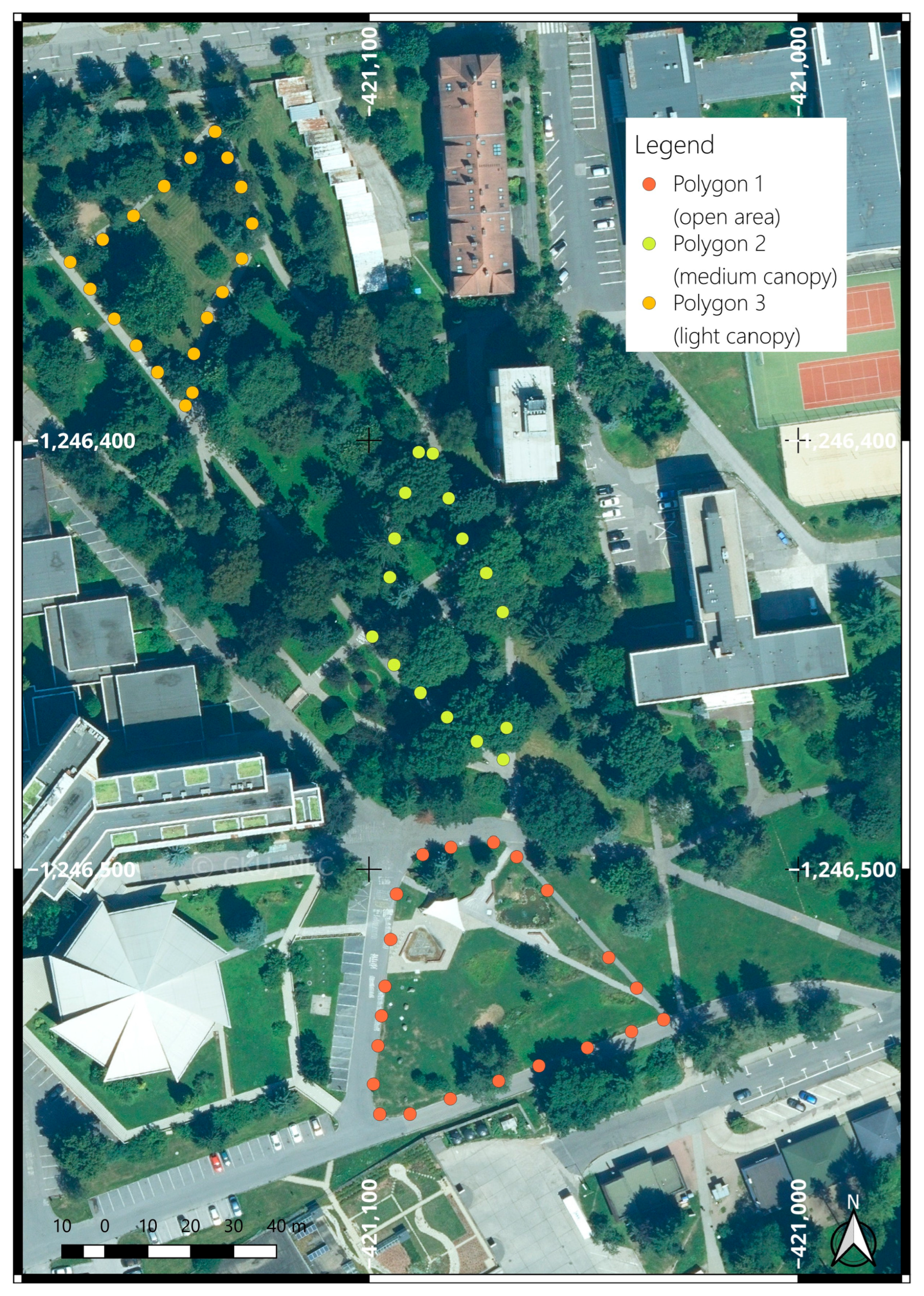
The study area was a park located near the Technical University in Zvolen, where three test polygons were established (Figure 1). Polygon No. 1 consisted of 21 reference points, all but one of which were free from direct tree canopy obstruction. Polygon No. 2 consisted of 17 reference points, almost all of which were completely obstructed by the surrounding trees. Within the experiment, this polygon represented conditions with the highest level of vegetation-induced obstruction, with numerous trees located in its immediate vicinity. Polygon No. 3 contained 19 test points, with a lower degree of vegetation obstruction compared to polygon No. 2. The surroundings of the measured polygons were dominated by deciduous tree species with diverse species composition.

The reference coordinates of the points were determined using a geodetic triple-frequency GNSS receiver, a Stonex S999 (Stonex, Paderno Dugnano, Italy), during the leaf-off period. The coordinates of points located under tree canopy cover were additionally verified by measurements carried out with a Topcon GPT9000 (Topcon, Tokyo, Japan) total station. The test points were stabilized in the field using geodetic nails and marked with reflective paint.

2.2. Data Collection

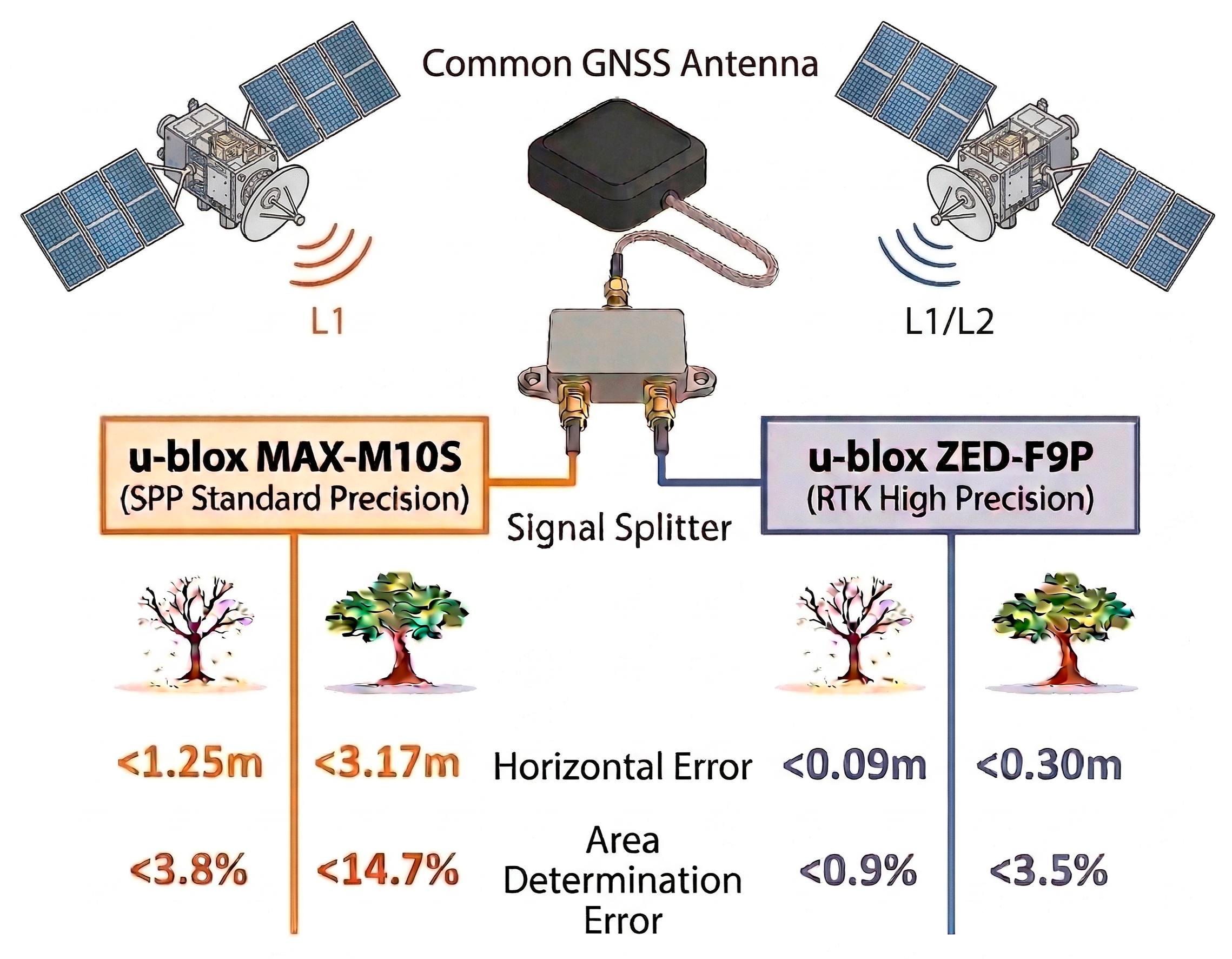
The measurement of the selected polygons at the study site was carried out using a measurement setup whose core consisted of two GNSS receivers—a u-blox ZED-F9P and a u-blox MAX-M10S. Both receivers represent modern low-cost GNSS devices; however, they differ in their supported frequencies and the ability to leverage GNSS corrections. This was the reason for their comparison under identical field conditions. The basic technical parameters of both receivers used in the experiment are presented in

Table 1. Technical parameters of the u-blox ZED-F9P and u-blox MAX-M10S GNSS receivers [28,29,30,31].

Specifications	SparkFun GNSS Receiver Breakout—MAX-M10S	u-blox C099-F9P
Module	MAX-M10S	ZED-F9P-01B-01
Module dimensions	9.7 × 10.1 × 2.5 mm	17.0 × 22.0 × 2.4 mm
Application board dimensions	44.2 × 30.5 mm	85 × 65 mm
Supported frequencies	L1	L1, L2
Supported systems and frequencies	GPS (L1C/A), GLONASS (L1OF), BeiDou (B1I/C), Galileo (E1-B/C)	GPS (L1C/A, L2C), GLONASS (L1OF, L2OF), BeiDou (B1I, B2I), Galileo, (E1B/C, E5b)
Autonomous horizontal accuracy	±1.5 m	±1.5 m
RTK accuracy	Not supported	0.01 m
NTRIP client	Not supported	Supported (via additional device)
Raw data logging	Not supported	Supported (UBX format, export to RINEX possible)
Supported protocols	NMEA, UBX	NMEA, UBX, RTCM
Year of module release	2022	2018
Price	50 €	230 €

.

Both GNSS receivers were connected to a shared dual-frequency u-blox ANN-MB-00-00 antenna via a signal splitter. The technical specifications for this antenna are detailed in

Table 2. Technical parameters of the u-blox ANN-MB-00-00 GNSS antenna [32].

Specifications	u-blox Dualband (L1/L2/E5b/B2I) GNSS Antenna
Model	u-blox ANN-MB-00-00
Type	Active GNSS antenna
Frequency bands	Dual-frequency: L1, L2/E5b/B2I
Supported constellations	GPS, GLONASS, Galileo, BeiDou
Frequency range	1559–1606 MHz and 1197–1249 MHz
Size	60 × 82 × 22.5
Price	50 €

. In addition to a cable with an SMA connector, the unit features two mounting holes for secure installation and an integrated magnet for attachment to metallic surfaces.

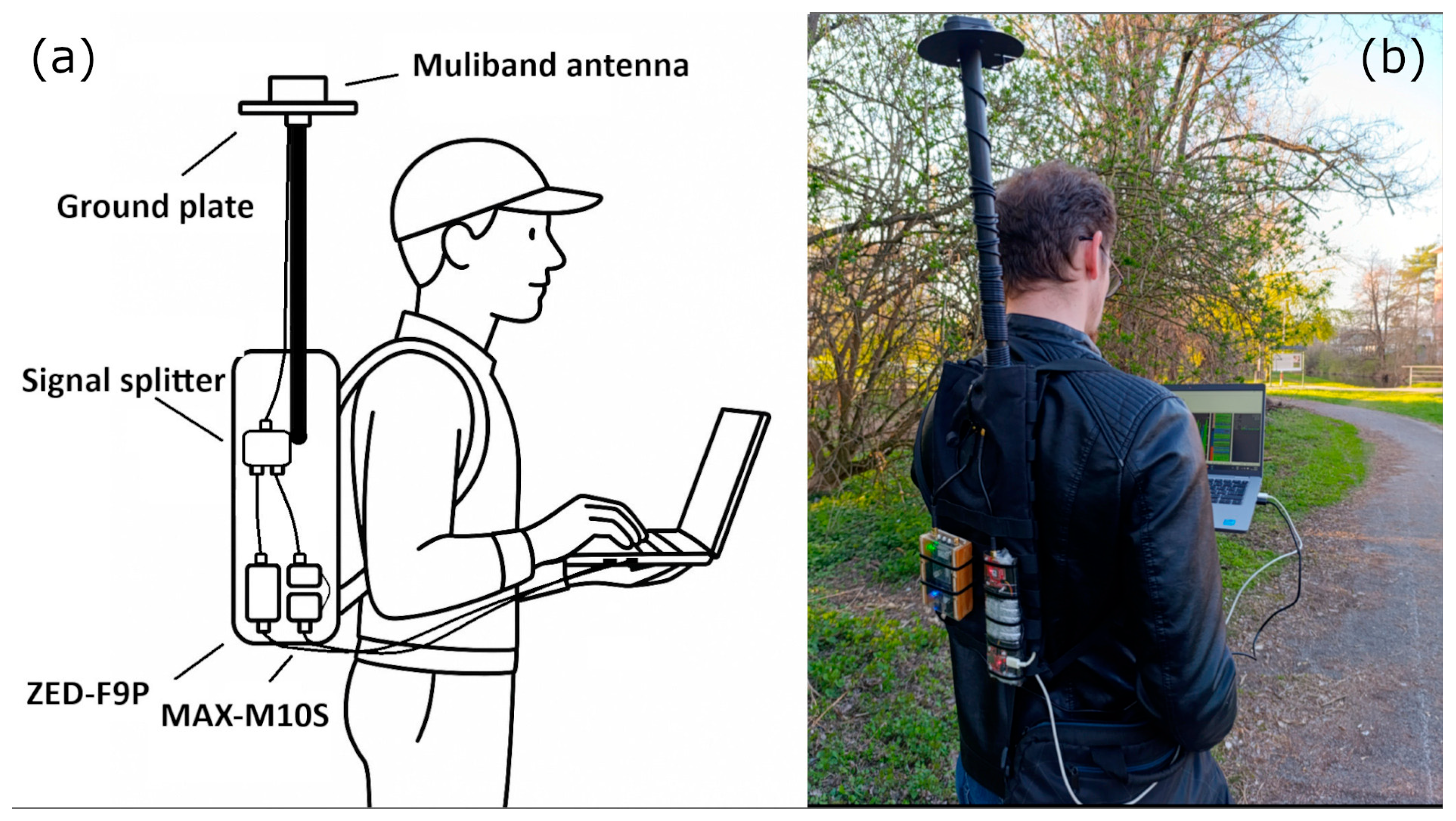
To simulate the practical use of GNSS receivers under real field conditions, both receivers, together with a signal splitter and antenna, were mounted on a backpack worn by the operator. The GNSS antenna was positioned above the operator’s head on a vertical support pole equipped with a ground plane, which contributed to mitigating the multipath effects and signal obstruction caused by the operator’s body (Figure 2). The total cost of the measurement setup was approximately 420€.

The receivers were connected to a laptop via USB cables, which was used for data logging and real-time monitoring of the measured data. Both devices recorded the positioning solution at a frequency of 1 Hz. The measurements were performed simultaneously, and the use of a common antenna ensured comparable satellite signal reception conditions. The signal was distributed to both receivers using a passive two-way GNSS splitter (ArduSimple GNSS Antenna Signal Splitter) operating in a 1.1–1.7 GHz frequency band. According to the manufacturer’s specifications, the splitter introduces a maximum power loss of 3.5 dB and a maximum signal-to-noise ratio degradation of 0.5 dB.

The data collection methodology applied in the case of the u-blox ZED-F9P corresponded to the principle of real-time kinematic (RTK) GNSS surveying, whereas in the case of the u-blox MAX-M10S, it corresponded to autonomous single-point positioning (SPP). At each measured point, the operator stopped for approximately 5 s, during which the receivers recorded five position estimates for the given point. In this way, a cluster of data was created around each point, enabling the subsequent identification of individual points and the averaging of multiple observations in order to improve the accuracy of the determined position. This methodology was adopted because none of the software tools used for data logging provided the option to store the position of an individual point at a specific time instant. The measurements taken with the u-blox ZED-F9P receiver were recorded using u-center 25.06 (u-blox AG, Thalwil, Switzerland) software in the raw data format of the UBX protocol, as well as in the standard NMEA protocol. The measurements obtained with the u-blox MAX-M10S receiver were recorded using the Tera Term Pro terminal in the NMEA 0183 format.

The individual measurement campaigns were conducted during two periods—during the vegetation (leaf-on) period, when the trees were in full foliage, and during the non-vegetation (leaf-off) period, when the foliage had fallen. To verify the repeatability of the achieved results and to increase their statistical robustness, five measurements were carried out on each polygon within each of these periods. During the leaf-on period, the measurements were conducted on 11, 18, 21, 24, and 25 October 2024. During the leaf-off period, measurements were performed on 3 February (morning), 3 February (afternoon), 4 February, 5 February, and 10 February 2025.

The correction data were provided by the TUZVO_ARB_SK reference station. The station was established within the Borová hora Arboretum for research purposes in the field of GNSS technologies. Its distance (baseline) from the study area where the measurements were conducted is 2.7 km.

The technical core of the station consists of a triple-frequency GNSS receiver, a simpleRTK 3B Pro, based on the Septentrio mosaic-X5 GNSS module, and a calibrated triple-frequency antenna. The detailed technical parameters are provided in

Table 3. Technical parameters of the simpleRTK 3B Pro GNSS receiver [33].

Specifications	SimpleRTK3B Pro
Module	Septentrio mosaic-X5
Module dimensions	31 × 31 × 4 mm
Application board dimensions	62 × 85 mm
Supported frequencies	L1, L2, L5
Supported systems	GPS (L1C/A, L2C, L5), Galileo (E1, E5a, E5b), GLONASS (L1OF, L2OF), BeiDou (B1I, B2I, B3I)
Autonomous horizontal accuracy	<1.5 m
RTK accuracy	0.01 m
NTRIP client	Supported (via additional device)
Raw data logging	Supported (RINEX, binary formats)
Supported protocols	NMEA, RTCM, SBF, RINEX

.

The station provides correction data in RTCM (MSN7) format for real-time measurements via the free RTK2GO service. At the same time, it generates and archives daily RINEX files with a 60 s interval, which are used for the post-processing and long-term monitoring of GNSS data. The u-blox ZED-F9P receiver received real-time correction data from this station through an NTRIP client, with the required internet connection provided by a mobile device.

A dataset, consisting of raw data (NMEA format for u-Blox MAX-M10S; UBX/NMEA format for uBloxZED-F9P) and reference data in Geopackage format are available in the Supplementary Material (Dataset S1).

2.3. Data Processing

For the purpose of data processing, reference coordinates in different coordinate systems were used for the individual receivers, depending on the positioning method applied. In the case of the u-blox ZED-F9P receiver, which was used for relative positioning, the reference coordinates were defined in the ETRS89 coordinate system in the ETRF2000 realization (epoch 2008.5), corresponding to the national coordinate reference standard used in Slovakia. This coordinate frame is used also by the TUZVO_ARB_SK station and for the reference coordinates of the points.

For the u-blox MAX-M10S receiver, intended for autonomous positioning, the coordinates were recorded in the WGS84 coordinate system, and for transformation of reference coordinates we used the ITRF2020 coordinate frame. The transformation between the ITRF2020 and ETRF2000 coordinates was conducted using the ETRF/ITRF Coordinate Transformation Tool [34].

The export of data from both receivers into CSV format was carried out within the u-center 25.06 (u-blox AG, Switzerland) environment. The exported file contained the latitude and longitude, ellipsoidal height, and a list of satellites in view and their total number. These CSV files were subsequently imported into QGIS 3.40.14 (QGIS Development Team, Switzerland) as delimited text layers, where further processing and evaluation were performed.

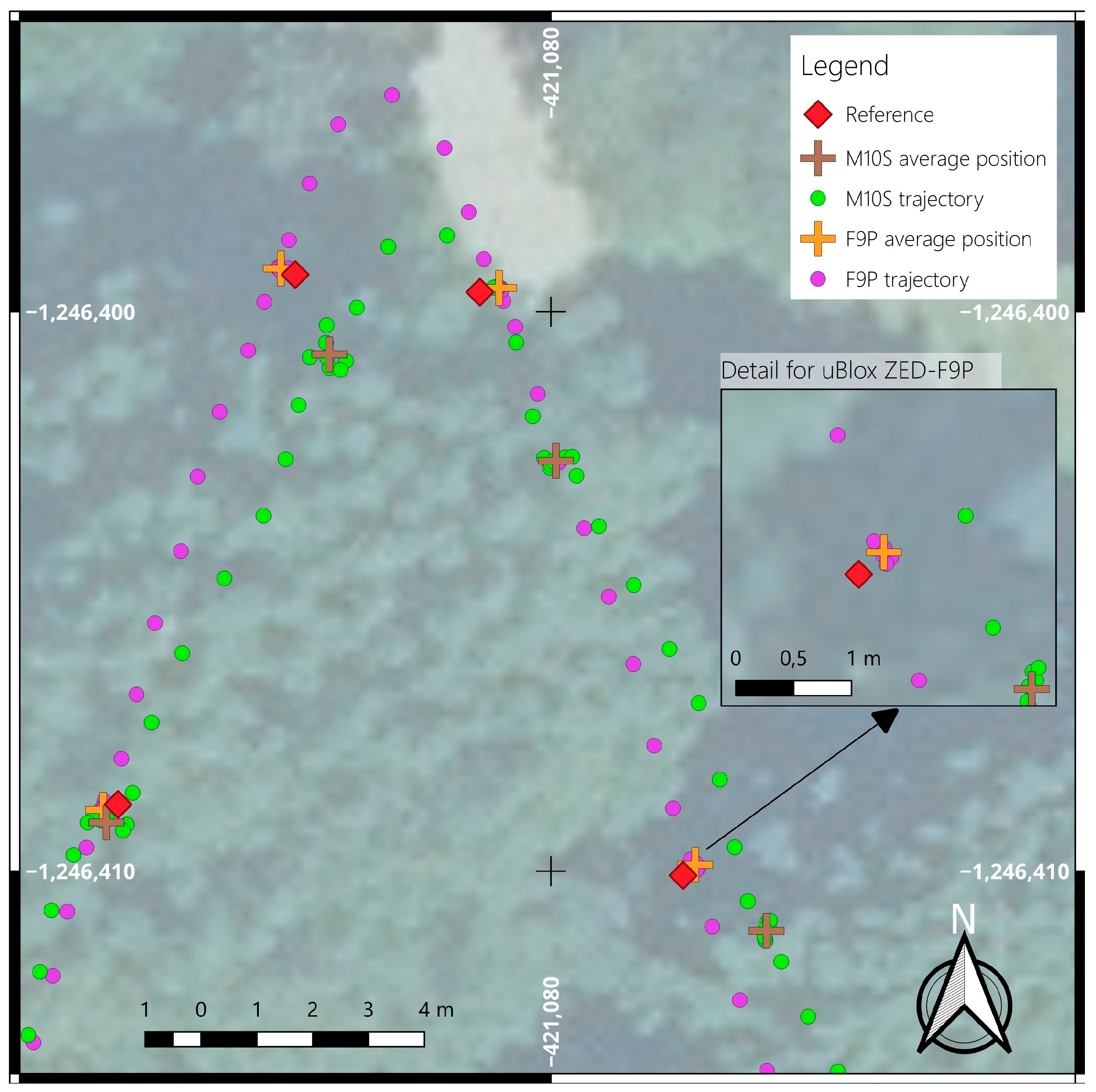
In the next stage of data processing, clusters of positions representing the 5 s stop at each point were selected, and their mean coordinates were calculated using the Mean Coordinates tool (Figure 3). These averaged coordinates were used as the final point position for the computation of horizontal errors relative to the reference coordinates. This procedure was applied to each individual measurement record, defined by the combination of the measurement date and the receiver used.

2.3.1. Calculation of Horizontal Errors

After creating layers containing the mean coordinates of the measured points, the horizontal error was calculated for each point relative to its corresponding reference point with the same identifier. The calculation was performed as the Euclidean distance between pairs of homologous points using the Distance Matrix tool implemented in QGIS.

The Euclidean distance between the measured point $i$ with coordinates $\left(x_i^m; y_i^m\right)$ and the reference point $i$ with coordinates $(x_i^r; y_i^r)$ was computed using the following Formula (1):

$$d_i= \sqrt{{(x_i^m-x_i^r)}^2+{(y_i^m-y_i^r)}^2}$$

(1)

where $d_i$ represents the horizontal error of point $i$, $x_i^m;y_i^m$ is the coordinate of the measured point and $x_i^r;{\mathrm{a}\mathrm{n}\mathrm{d} y}_i^r$ is the coordinate of the corresponding reference point.

As a final step, the results of the coordinate differences were exported to MS Excel, where the mean distance and standard deviation were calculated for each record. The maximum and minimum values were also determined. These results were subsequently consolidated into summary tables and figures.

A statistical analysis, conducted using Statistica 14 software (TIBCO Software Inc., San Ramon, CA, USA), included a factorial ANOVA focused on effects of receiver, season, conditions, and their combinations on the horizontal errors. The pairwise differences were evaluated using a post hoc Tukey HSD test. Regarding the quantitative/qualitative characteristic of acquired data, the correlation between the horizontal errors and the number of visible satellites, signal-to-noise density, and positional dilution of precision was determined.

2.3.2. Calculation of Area Differences

To assess the possibility of area determination, lines were generated from the coordinates of the reference points and the averaged measured points using the Point to Path tool. These lines were subsequently converted into polygon features using the Line to Polygon module, resulting in reference and measured polygons.

The areas of the reference polygons were determined as follows: polygon No. 1 had an area of 2610.8 m², polygon No. 2 an area of 1256.4 m², and polygon No. 3 an area of 1253.8 m². The areas of the generated polygons were then compared to quantify the differences between the reference values and the data obtained from the individual measurements.

3. Results

3.1. Results of Measurements Using u-blox ZED-F9P

The horizontal errors of the u-blox ZED-F9P receiver during the vegetation period are summarized in

Table 4. Averages and standard deviations of horizontal errors (in meters) for the u-blox ZED-F9P during the leaf-on period.

Measurement Num.	Pol.1 (Open Area)	Pol.2 (Medium Canopy)	Pol.3 (Light Canopy)
1 (11 October 2024)	0.078 ± 0.031	0.304 ± 0.054	0.210 ± 0.063
2 (18 October 2024)	0.118 ± 0.030	0.140 ± 0.074	0.159 ± 0.031
3 (21 October 2024)	0.108 ± 0.033	0.153 ± 0.038	0.210 ± 0.062
4 (24 October 2024)	0.150 ± 0.054	0.185 ± 0.066	0.185 ± 0.038
5 (25 October 2024)	0.090 ± 0.032	0.114 ± 0.045	0.096 ± 0.033
Overall	0.109 ± 0.036	0.179 ± 0.055	0.172 ± 0.045

. The lowest horizontal errors were observed in the open area (polygon No. 1), where the positioning accuracy remained relatively stable throughout the monitoring period. The overall minimum recorded horizontal error was 0.015 m, whereas the maximum horizontal error reached 0.288 m.

Under a medium canopy (polygon No. 2), the errors were noticeably higher and showed greater variability compared to the open area, indicating the influence of vegetation on signal quality. The minimum recorded error for this polygon was 0.012 m, while the maximum value reached 0.430 m.

The measurements performed under conditions with a light vegetation canopy (polygon No. 3) resulted in horizontal errors that were generally higher than those in the open area but slightly lower than those observed under medium-canopy conditions. The lowest recorded error was 0.047 m, whereas the maximum horizontal error reached 0.423 m.

Overall, the results obtained during the leaf-on period indicated that the minimum errors across all polygons remained below 0.05 m, while the maximum horizontal errors reached 0.43 m.

The horizontal errors of the u-blox ZED-F9P receiver during the leaf-off period are presented in

Table 5. Averages and standard deviations of horizontal errors (in meters) for the u-blox ZED-F9P during the leaf-off period.

Measurement Num.	Pol.1 (Open Area)	Pol.2 (Medium Canopy)	Pol.3 (Light Canopy)
1 (3 February 2025 AM)	0.075 ± 0.035	0.071 ± 0.043	0.079 ± 0.039
2 (3 February 2025 PM)	0.072 ± 0.040	0.084 ± 0.045	0.091 ± 0.021
3 (4 February 2025)	0.096 ± 0.060	0.099 ± 0.044	0.069 ± 0.039
4 (5 February 2025)	0.051 ± 0.034	0.055 ± 0.040	0.042 ± 0.039
5 (10 February 2025)	0.065 ± 0.037	0.060 ± 0.025	0.075 ± 0.039
Overall	0.072 ± 0.041	0.074 ± 0.039	0.071 ± 0.035

. For polygon No. 1, the mean horizontal errors remained relatively low and stable throughout the individual measurements. The minimum observed horizontal error was 0.008 m, whereas the maximum horizontal error reached 0.282 m. For polygon No. 2, the horizontal errors were comparable to those observed in polygon No. 1, although slightly higher variability was recorded for some measurements. The minimum observed horizontal error for this polygon was 0.009 m, while the maximum horizontal error reached 0.181 m. Polygon No. 3 showed horizontal errors similar to those of the other polygons, with relatively stable results across the monitored period. The minimum observed horizontal error was 0.008 m, whereas the maximum horizontal error reached 0.188 m. Overall, the minimum horizontal error across all polygons was 0.009 m, whereas the maximum horizontal error reached 0.29 m. Surprisingly, the post hoc Tukey HSD test (Table S1, available in the Supplementary Material) did not identify any significant pairwise differences for this receiver.

Determination of Areas Using the u-blox ZED-F9P Receiver

The relative differences in the polygon areas identified during both monitored periods are presented in

Table 6. Relative differences in polygon areas (%) between measured and reference polygons during both periods using the u-blox ZED-F9P.

Measurement Num.	Leaf-On			Leaf-Off
	Pol.1	Pol.2	Pol.3	Pol.1	Pol.2	Pol.3
1	0.4	3.5	2.7	0.4	0.2	0.2
2	0.6	0.8	1.5	0.3	0.6	0.9
3	0.6	1.7	2.2	0.3	0.8	0.3
4	0.9	1.8	1.9	0.0	0.0	0.0
5	0.4	1.1	1.0	0.1	0.4	0.5
Overall	0.6	1.8	1.8	0.2	0.4	0.4

. The table summarizes the percentage differences between the individual repeated measurements, as well as their mean values, allowing for a clear comparison of result stability between the leaf-on and leaf-off periods.

During the leaf-on period, higher area differences were recorded across all monitored polygons. The maximum absolute differences reached 24.3 m² for the open-area polygon (No. 1), 45.7 m² for the medium-canopy polygon (No. 2), and 34.6 m² for the light-canopy polygon (No. 3), corresponding to relative differences of approximately 0.9%, 3.5%, and 2.7%, respectively. The mean percentage differences during this period were approximately 0.6% for polygon No. 1 and 1.8% for polygons No. 2 and No. 3.

After leaf fall, the area differences decreased. The maximum difference for polygon No. 1 was 10.0 m² (0.4%), 9.7 m² (0.8%) for polygon No. 2, and 11.5 m² (0.9%) for polygon No. 3.

In terms of the direction of the differences, the calculated areas were consistently higher than the reference values across all test locations. All the identified differences were positive, resulting in higher calculated area values for the individual repeated measurements. This trend was particularly pronounced for polygons No. 2 and No. 3, where the highest percentage differences were recorded.

After leaf fall, the calculated areas remained higher than the reference values; however, the differences were substantially smaller. The observed differences were markedly lower compared to the leaf-on period and remained at the level of tenths of a percent. Despite the persistently positive direction of the differences, no pronounced deviations were recorded between the individual repeated measurements during this period.

3.2. Results of Measurements Using u-blox MAX-M10S

For the measurements conducted using the u-blox MAX-M10S receiver, significant deviations and errors were identified for both monitored periods, clearly exceeding the typical range of the observed results. Specific cases are listed in

Table 7. Summary of measurements exhibiting excessive errors from the u-blox MAX-M10S receiver.

Period	Date	Polygon No.	Error Characteristics
Leaf-on	25 October 2024	1	Unusually large horizontal errors.
	24 October 2024	3	Failure of trajectory closure.
	11 October 2024	2	Unusually large horizontal errors.
Leaf-off	4 February 2025	2	Missing parts of the trajectory, including two test points.

, together with a brief description of their characteristics. Even a detailed analysis of the parameters recorded in the NMEA messages (number of visible satellites, C/N0, PDOP) did not identify a sound reason for these discrepancies. These cases were included in the calculations and subsequently influenced the final results, thereby affecting the interpretation of measurement accuracy on the respective days, as well as the overall average summary results. However, if possible, we also report the results excluding these extremes.

During the leaf-on period (

Table 8. Averages and standard deviations of horizontal errors (in meters) for the u-blox MAX-M10S during the leaf-on period.

Measurement Num.	Pol.1 (Open Area)	Pol.2 (Medium Canopy)	Pol.3 (Light Canopy)
1 (11 October 2024)	1.190 ± 0.386	2.430 ± 1.493	0.902 ± 0.433
2 (18 October 2024)	0.536 ± 0.055	0.660 ± 0.248	1.451 ± 0.340
3 (21 October 2024)	1.984 ± 0.483	0.998 ± 0.499	0.908 ± 0.338
4 (24 October 2024)	1.090 ± 0.402	2.847 ± 0.939	3.055 ± 0.909
5 (25 October 2024)	3.171 ± 0.996	2.168 ± 0.610	1.730 ± 0.974
Overall	1.594 ± 0.465	1.821 ± 0.758	1.609 ± 0.599

), the horizontal errors of the u-blox MAX-M10S receiver in the open-area polygon (No. 1) showed substantial variability among the individual measurement sessions. The minimum horizontal error was 0.366 m, whereas the maximum horizontal error reached 5.312 m. Particular attention should be given to the mean horizontal error of 3.171 m observed for the fifth measurement on 25 October 2024, which represents the highest recorded error across all measurement datasets, including those acquired under tree canopy conditions. No clear explanation for this deviation was identified. When this value was excluded from the evaluation, the average horizontal error for the measurements conducted in open-area conditions decreased to approximately 1.2 m.

For polygon No. 2, with a medium vegetation canopy, the horizontal errors were generally higher and more variable than in the open area. The minimum horizontal error recorded for this polygon was 0.227 m, whereas the maximum horizontal error reached 5.496 m.

The light-canopy polygon No. 3 exhibited horizontal errors comparable to those observed under medium-canopy conditions. The minimum horizontal error recorded was 0.103 m, whereas the maximum horizontal error reached 4.819 m.

Overall, the minimum recorded errors across all polygons remained below 0.5 m, whereas the maximum errors exceeded 5 m.

During the leaf-off period (

Table 9. Averages and standard deviations of horizontal errors (in meters) for the u-blox MAX-M10S during the leaf-off period.

Measurement Num.	Pol.1 (Open Area)	Pol.2 (Medium Canopy)	Pol.3 (Light Canopy)
1 (3 February 2025 AM)	0.952 ± 0.305	0.768 ± 0.287	0.836 ± 0.422
2 (3 February 2025 PM)	0.469 ± 0.360	0.712 ± 0.504	0.836 ± 0.422
3 (4 February 2025)	0.934 ± 0.227	0.792 ± 0.308	0.902 ± 0.297
4 (5 February 2025)	1.025 ± 0.227	0.994 ± 0.676	1.255 ± 0.370
5 (10 February 2025)	1.247 ± 0.413	0.871 ± 0.535	0.903 ± 0.414
Overall	0.925 ± 0.306	0.827 ± 0.462	0.946 ± 0.385

), the average horizontal errors of the u-blox MAX-M10S receiver in open-area conditions remained relatively stable across the individual measurement sessions. The minimum horizontal error reached 0.007 m, whereas the maximum horizontal error reached 2.018 m.

For polygon No. 2, the horizontal errors were comparable to those observed in the open-area conditions, although higher variability was observed for some measurements. The minimum horizontal error recorded for this polygon was 0.022 m, while the maximum horizontal error reached 2.692 m. The measurements conducted in polygon No. 3 exhibited horizontal errors similar to those observed in the other polygons. The minimum horizontal error was 0.125 m, whereas the maximum horizontal error reached 1.880 m. The minimum recorded values across all polygons did not exceed 0.13 m, while the maximum horizontal errors reached up to 2.7 m.

A post hoc Tukey HSD test (Supplementary Table S1) showed significant differences between seasons (leaf on, leaf off). However, none of the significant differences were pronounced for differing measurement conditions (open area, medium and light canopy) within the seasons.

Determination of Areas Using the u-Blox MAX-M10S Receiver

The identified relative differences between the reference and measured polygon areas during both periods are summarized in

Table 10. Relative differences in polygon areas (%) between measured and reference polygons during both periods using the u-blox MAX-M10S.

Measurement Num.	Leaf-On			Leaf-Off
	Pol.1	Pol.2	Pol.3	Pol.1	Pol.2	Pol.3
1	1.4	14.7	4.1	1.5	2.8	1.6
2	0.0	1.5	1.8	1.7	1.7	3.8
3	3.5	1.5	1.5	−2.2	−0.9	−2.3
4	2.1	6.2	−2.4	1.3	−0.5	1.3
5	−4.0	−10.8	1.2	−0.5	−3.1	−0.8
Overall	0.6	2.6	1.2	0.4	0.0	0.7

. The table presents the percentage differences for individual measurements, as well as their average values, enabling a clear comparison of results between the leaf-on and leaf-off periods.

For polygon No. 1, the largest area difference reached −100.3 m² (4.0%). For polygon No. 2, the recorded differences reached up to 216.6 m² (14.7%). For polygon No. 3, the highest absolute difference amounted to 53.3 m² (4.1%).

Table 10 further presents the differences between the reference and measured polygon areas during the leaf-off period. For polygon No. 1, the largest absolute area difference was −58.1 m², corresponding to an underestimation of 2.2%. In the case of polygon No. 2, the maximum absolute difference reached −40.2 m² (3.1%). For polygon No. 3, the largest absolute difference was 48.2 m², indicating that the measured polygon area was 3.8% larger than the reference value.,

With respect to the direction of the relative differences, both the overestimation and underestimation of polygon areas relative to the reference values were observed for both periods. Thus, the overall mean values are not considered representative. The direction of the differences was not consistent, as positive and negative values alternated across the repeated measurements. This pattern was preserved in both the leaf-on and leaf-off periods and is different from the ZED-F9P results, where all the differences were positive.

3.3. Overall Summary and Comparison of Horizontal Errors

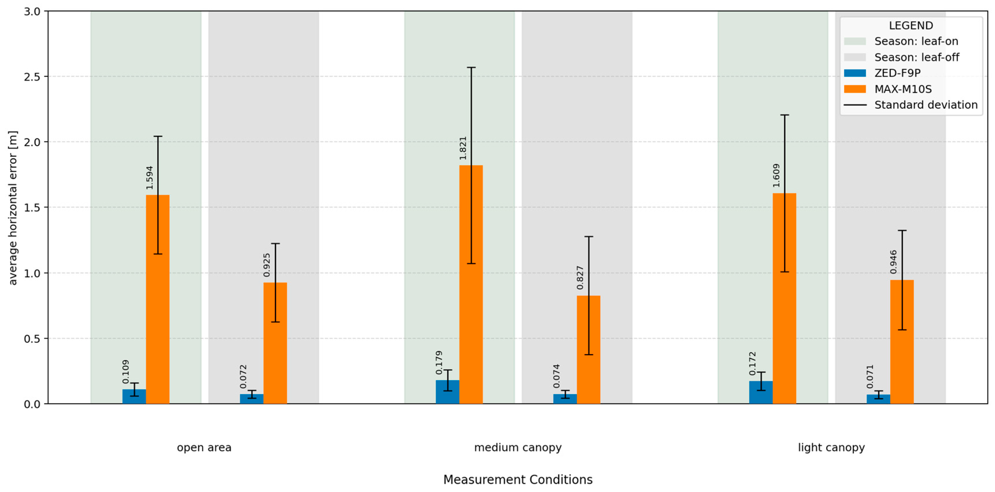
Figure 4 presents a summary overview of the average horizontal errors of both tested GNSS receivers across the individual polygons during the leaf-on and leaf-off periods. The displayed values represent the means obtained from repeated measurements, complemented by standard deviations that express the variability in the individual measurements.

In all evaluated cases, the u-blox ZED-F9P receiver achieved a lower average horizontal error than the u-blox MAX-M10S, regardless of canopy conditions or vegetation period. The mean values for the u-blox ZED-F9P ranged approximately between 0.07 m and 0.18 m, whereas the u-blox MAX-M10S exhibited an average error of approximately 0.8 m to 1.8 m. This difference was consistent across all three polygons.

In addition to its performance at the test points, the ZED F9P provided a more stable positional solution and continuous device trajectory. On the other hand, the trajectories acquired by the MAX-M10S receiver suffered from discontinuities or position jumps in several cases. This could present a practical issue in applications where the trajectory stability is of higher priority.

A comparison of the leaf-on and leaf-off periods revealed a decrease in the average horizontal error for both receivers following leaf fall. This reduction was evident across all canopy conditions, with the difference between the two vegetation periods being more pronounced for the u-blox MAX-M10S. A concurrent decrease in the standard error was also observed during the leaf-off period, indicating lower variability in the measurement results. The graphical comparison presented in Figure 4 provides a clear overview of the differences in positioning accuracy between the receivers, the influence of vegetation conditions on the measurement results, and the stability of measurements across the individual polygons.

3.4. Factors Influencing Horizontal Accuracy

Table 11. Results of three-way factorial ANOVA for effects of receiver, season and conditions on horizontal error. Significant effects are marked with italics.

Effect	Sum of Squares	Degrees of Freedom	Mean Square	F	p
Receiver	388.4848	1	388.4848	1114.719	0.000000
Season	52.0300	1	52.0300	149.295	0.000000
Conditions	0.5027	2	0.2514	0.721	0.486375
Receiver × Season	33.6948	1	33.6948	96.684	0.000000
Receiver × Conditions	0.1011	2	0.0505	0.145	0.865055
Season × Conditions	1.9976	2	0.9988	2.866	0.057343
Receiver × Season × Conditions	1.3548	2	0.6774	1.944	0.143645
Intercept	554.3533	1	554.3533	1590.663	0.000000
Error	392.4162	1126	0.3485

summarizes the results of the analysis regarding the factors influencing the horizontal error. The three-way factorial ANOVA considered the receiver type, season, measurement conditions, and their interactions. The analysis revealed that the main effects of receiver and season, along with their two-way interaction, were the only statistically significant effects. The importance of receiver selection was anticipated, as the F9P and M10S represent different grades of low-cost receivers utilizing distinct positioning methods. The season also severely impacted the accuracy; specifically, the presence of canopy foliage played a major role, with the results acquired during the leaf-off season being significantly better. The significant interaction between receiver and season indicates that the F9P coped with the foliage much better than the M10S. Surprisingly, the main effect of measurement conditions (open area vs. under canopy) was not significant. This is presumably related to the results acquired during the leaf-off season, where the differences between the open-area and under-canopy conditions were negligible, thereby diluting the overall effect. This presumption is further supported by the interaction between the season and conditions, which approached statistical significance (p = 0.057).

The analysis of quantitative/qualitative characteristics of acquired GNSS signals is limited by the NMEA 0183 format as this is the only format used by the M10S receiver. It provides only information on number of satellites, signal-to-noise density (C/N0) and positional dilution of precision (PDOP), with further restrictions debated in parts related to particular characteristics. The NMEA format reports two satellite counts: visible and used. However, because the “used” satellite count is capped at 12, both receivers consistently reported a value of 12 across all test scenarios. 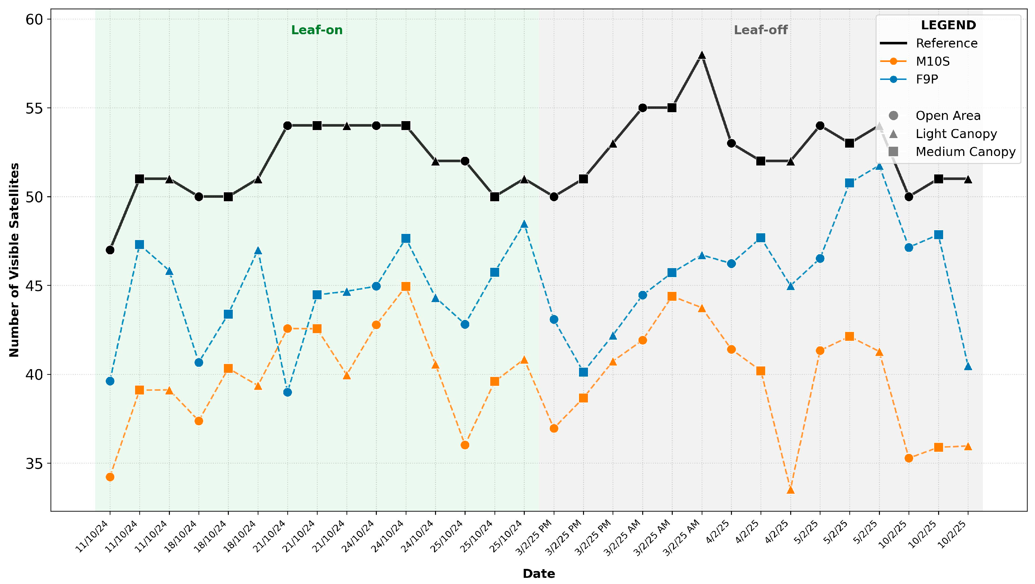Figure 5 illustrates the number of visible satellites for both receivers compared to the theoretical count generated by Trimble GNSS Planning [35] (no elevation cut-off angle was applied). In all but one of the 30 measurements, the ZED-F9P receiver detected more visible satellites than the MAX-M10S. On average, the ZED-F9P tracked five more satellites (45 vs. 40). Compared to the theoretical reference count, the F9P fell short by an average of seven satellites, while the M10S fell short by 12. The seasonal variations had a negligible impact on these numbers. The M10S averaged 40 visible satellites across both seasons, whereas the F9P averaged 44 during the leaf-on period and 46 during leaf-off period. For context, the theoretical reference averages differed by only one satellite between seasons (52 for leaf on vs. 53 for leaf off). Similarly, the specific measurement conditions showed no clear trend; unexpectedly, the lowest satellite counts were recorded on several dates under open-sky conditions. The positional dilution of precision (PDOP) closely correlates with satellite availability. The M10S and F9P receivers averaged excellent PDOP values of 0.95 and 0.97, respectively—both fully sufficient for a successful positioning solution. Overall, while both receivers benefited from a high number of visible satellites and good geometry, the NMEA format was not able to provide usable information regarding the specific satellites used in the positional solution.

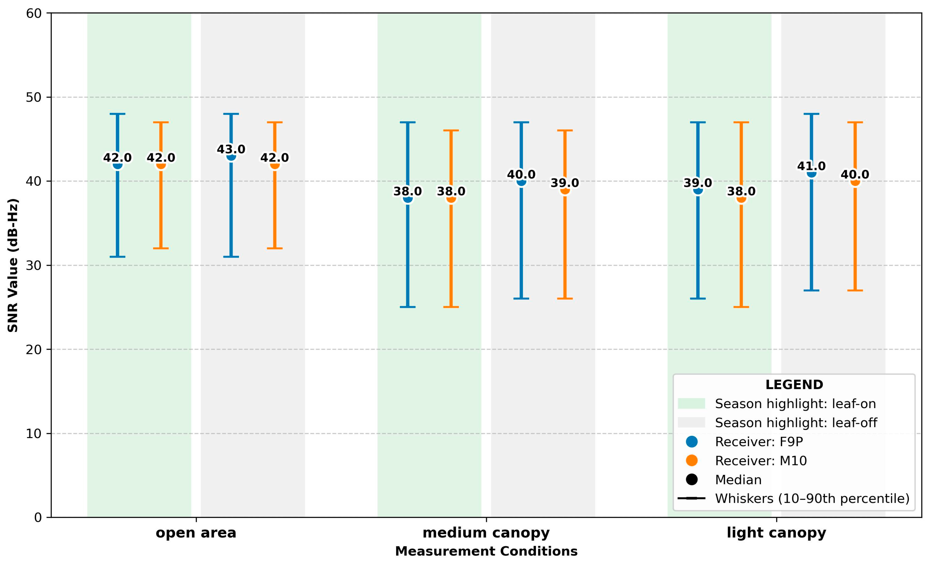
Another limitation of using NMEA 0183 is that the format only provides the signal-to-noise density (CN/0) for the GPS L1 signal, and it is in integer values. The analysis reveals that while both the F9P and M10S receivers performed optimally and with minimal variance in the open-area conditions (maintaining median values around 42–43 dB-Hz regardless of the season), the introduction of vegetation canopy significantly degraded the signal quality and increased the variability (Figure 6). The density of the vegetation played a crucial role; both the light- and medium-canopy environments showed distinct signal attenuation, which was notably exacerbated during the leaf-on season. For instance, transitioning from leaf-off to leaf-on conditions under canopy conditions dropped the median C/N0 by approximately 2 dB-Hz. Furthermore, a clear performance distinction emerged in the obstructed environments, where the F9P receiver consistently outperformed the M10S, maintaining higher median C/N0 values and demonstrating slightly better resilience to the signal interference caused by vegetation. However, the differences were at the rate of only 1dB-Hz. This can be partially accounted for by the use of common antenna.

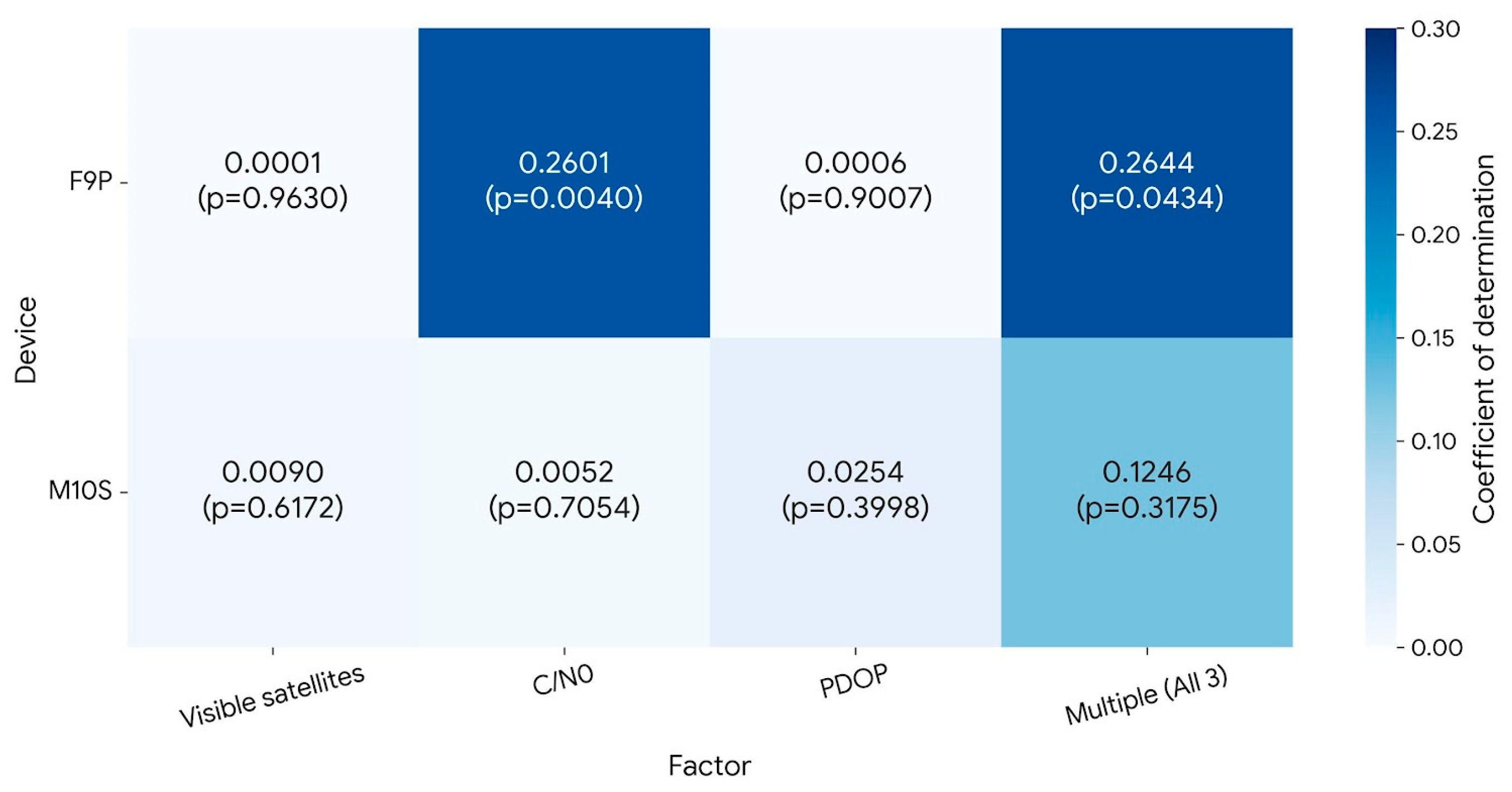
The statistical analysis of the correlation between the mentioned characteristics and the horizontal errors revealed the distinct sensitivities of the evaluated receivers (Figure 7). For the F9P, the signal-to-noise density (C/N0) was the only statistically significant individual predictor of spatial accuracy (p < 0.01), explaining approximately 26.0% of the error variance (R² = 0.2601). A multiple linear regression model incorporating the C/N0, PDOP, and the number of satellites yielded only a marginal increase to a Multiple R² of 0.2643, indicating that the additional parameters provided no meaningful explanatory value beyond signal attenuation for this device. Conversely, the M10S receiver exhibited no strong individual correlations, with the PDOP yielding the highest independent coefficient of determination at merely 2.5% (R² = 0.0254, p > 0.05). However, the multi-factor model for the M10S revealed a notable additive effect, successfully explaining 12.4% of the error variance when all three parameters were evaluated concurrently. These results suggest that while the F9P’s error variations are primarily driven by direct signal strength, the positioning error of the M10S is influenced by a more complex, albeit moderate, interaction of satellite geometry, availability, and signal quality. Generally, the monitored factors describe only a marginal part of the positional error variance.

4. Discussion

The presence of tree vegetation, particularly during the full leaf-on period, represents a significant negative factor affecting positioning accuracy. Although this effect has been documented since the early availability of GNSS for civilian applications [10,23,36], the tested low-cost receivers—the u-blox ZED-F9P and u-blox MAX-M10S—responded differently to these conditions, despite sharing a common antenna. This highlights the differing capabilities of the individual devices in coping with limited satellite signal reception.

Before interpreting the findings, several methodological aspects should be considered. In the mobile measurement setup, the GNSS antenna was positioned on the operator’s back, which may not have always ensured perfect centering above the measured point, and could therefore represent a minor source of positioning uncertainty. However, all measurements were performed by the same operator, ensuring consistency in the antenna placement procedure throughout the data acquisition sessions. Furthermore, the experiments were conducted using a low-cost u-blox ANN-MB-00 patch antenna, which provides lower multipath suppression compared to survey-grade geodetic antennas [37], consistent with the low-cost configuration of the experiment. It is possible to get more advanced, calibrated low-cost antennas for a price of few hundred euros, but this means a significant increase in the price of the whole setup. The passive signal splitter used to connect both receivers to the antenna introduced a maximum power loss of approximately 3.5 dB, while the manufacturer specifies a maximum GNSS signal-to-noise ratio (SNR) degradation of about 0.5 dB. Such attenuation is generally not expected to significantly affect positioning accuracy, but it may have slightly reduced the signal robustness under the already degraded reception conditions. It should also be noted that the measurements represent a concurrent evaluation of the tested receivers in their typical operating configurations rather than a strict comparison of positioning algorithms under identical positioning modes. Regarding other adverse effects on the GNSS performance, the testing took place in autumn 2024 and early spring 2025, coinciding with the peak of the solar activity cycle. Although the ionospheric interference was presumably elevated during this period, we lack the long-term observational data necessary to quantify this effect. The adopted methodology—the simultaneous testing of two receivers connected to a common antenna and averaging clusters of positional estimates over a 5 s interval at each point—proved to be suitable and reliable for obtaining the representative coordinates. From a practical perspective, positioning the antenna on the operator’s back offers the advantage of hands-free operation, allowing for additional tasks to be performed concurrently with the measurements. Nevertheless, the mentioned limitation remains the difficulty in fully exploiting the achievable positioning accuracy, primarily due to the already mentioned ambiguity in precise antenna centering above the measured point.

4.1. Horizontal Positioning Accuracy

The dual-frequency u-blox ZED-F9P receiver, utilizing RTK differential corrections, demonstrated high solution stability and low horizontal errors under vegetation canopy conditions. Even during the full leaf-on period, the average errors recorded for the polygons located under canopy cover were lower than 0.20 m. This level of accuracy exceeds the results reported by Abdi et al. [6], who achieved an absolute deviation of 0.43 m in a forest environment using the same type of receiver and antenna. The observed difference is likely related to the varying complexity of the tested environments. The stability of the RTK solution is reflected in the receiver’s ability to maintain a fixed positioning solution during most measurements in both periods. This finding contrasts with the results reported by Ogundipe et al. [38], who documented difficulties in maintaining a fixed RTK solution under conditions of vegetation-induced signal obstruction. The RTK stability in our study was likely enhanced by the high satellite availability, averaging approximately 31 satellites per polygon. This substantially exceeds the values reported in the mentioned study, where the number of satellites ranged between 6 and 17. The increased satellite availability can be attributed not only to the measurement conditions themselves, but primarily to the inclusion of signals from the BeiDou satellite system, which were not utilized in the referenced study.

With respect to the changes in the horizontal errors following leaf fall, a 34% reduction in the mean deviation was observed for the open area (polygon 1). This unexpected improvement in accuracy was likely partially influenced by the surrounding vegetation, even though the measurement points had been established with consideration given to minimizing obstructions at higher satellite elevation angles. For the polygons affected by vegetation canopy, the improvement reached approximately 60% compared to full leaf-on conditions. A similar trend of enhanced accuracy outside the vegetation period was already reported in an earlier study by Žihlavník et al. [36], who observed a 47% improvement in the positioning accuracy when testing a geodetic-grade dual-frequency receiver. The average errors achieved during the leaf-off period across all polygons were approximately 0.07 m. This suggests that the remaining biomass (tree trunks and branches) had only a minimal influence on the positioning performance, and that the deterioration observed during the vegetation period was primarily attributable to the foliage. The maximum error of the u-blox ZED-F9P receiver did not exceed 0.5 m in either period, thereby meeting the requirements for the preparation of forestry maps in Slovakia [39].

The single-frequency u-blox MAX-M10S receiver operating without differential corrections demonstrated pronounced sensitivity to vegetation-induced signal obstruction, as reflected by the increased horizontal error and measurement errors. During the leaf-on period, the average horizontal error in open-area conditions slightly exceeded 1.5 m, thereby exceeding the manufacturer’s specified error margins for measurements under ideal conditions. In areas affected by vegetation canopy, the mean errors were higher; however, for polygon No. 3 the difference amounted to only 1 cm, which cannot be considered a significant difference. During this period, the maximum errors exceeded 4 m for all polygons. The average number of satellites in view across the polygons was 28. In contrast to the u-blox ZED-F9P, a higher frequency of extreme values and overall greater variability in the results were observed in this case. In several instances, short interruptions in position determination were also recorded.

Leaf fall resulted in a pronounced reduction in the average horizontal errors across all evaluated cases. In open-area conditions, the difference between the two periods reached 41%, which can again be attributed to the influence of surrounding vegetation. The most substantial improvement was observed for the polygon with the densest canopy cover, where the difference reached 54%, while for polygon No. 3, an improvement of 41% was recorded. Similarly to the previous receiver, the mean errors during the leaf-off period remained at a comparable level across all evaluated conditions (0.8–0.9 m). Notably, the lowest average error was observed for the polygon with the highest degree of canopy obstruction. This suggests that, under leaf-off conditions, the resulting positioning accuracy is influenced more by intrinsic receiver limitations and other environmental or operational factors than by the vegetation itself.

The average error achieved by the u-blox MAX-M10S, which remained approximately within 2 m even under degraded signal reception conditions, represents a better performance than that reported by Garrido-Carretero et al. [40]. In their testing of single-frequency GNSS devices, these authors reported average horizontal errors ranging from 4.75 m to 5.38 m. However, the maximum error from the reference trajectory was substantially higher in certain segments, reaching values between 9.38 m and 16.80 m.

In summary, the dual-frequency RTK receiver maintained sub-decimeter horizontal accuracy under both vegetation conditions, whereas the single-frequency standalone receiver showed meter-level errors and higher variability.

4.2. Accuracy of Area Determination

In natural resource management, one of the key tasks is the determination of area extent. In forestry, this typically involves assessing the size of areas designated for harvesting and post-harvest evaluation, territories affected by disturbances, and sites intended for reforestation. When maintaining the same level of positional accuracy of the applied method or instrument, the relative error of area determination decreases as the size of the area increases [26]. In our experiment, the assessed areas were relatively small, ranging from 0.13 to 0.26 ha. For such limited extents, the influence of the positional accuracy of the employed device becomes particularly critical and, in certain cases, may even prevent the determination of a reliable area value. Despite this, the maximum relative errors exceeded 10% only for two measurements during the leaf-on period with the u-blox MAX-M10S receiver under the most severe canopy conditions. In all other cases, the errors exceeded 5% only once, while the leaf-off period visibly reduced the variability in the results. Similarly to the evaluation of horizontal positioning accuracy, the results obtained with the u-blox ZED-F9P receiver were markedly superior. A 3% threshold was exceeded in only one instance, specifically for the measurements conducted under the most severe canopy conditions in the leaf-on period. For the measurements conducted in the open area, as well as under canopy conditions during the leaf-off period, the area differences determined by this receiver did not exceed 1%. From the perspective of practical application in forest environments, the conclusions reported by Ucar et al. [26] are particularly relevant. According to their findings, the method based on walking the perimeter of an area and recording points at predefined intervals represents an appropriate approach for data acquisition, even when using recreational single-frequency receivers without correction support. The areas examined in their study were substantially larger (approximately 9000 m² and above). Simulations based on error distribution indicate that for smaller extents (e.g., 1 ha), the relative deviation may reach up to 10%, whereas for larger areas (above 25 ha), it decreases to below 2%. In relation to the results obtained in our study, this may suggest that, when an appropriate methodology is applied, a receiver comparable to the u-blox MAX-M10S may achieve a level of accuracy sufficient for selected, less demanding applications. Area differences of up to 10% were also reported by Tomaštík et al. [18], where five mobile devices and a single-frequency mapping-grade receiver without correction support were used for area determination in forest environments during the leaf-on period. The assessed areas ranged from 2.1 to 5.8 ha.

A considerable proportion of tasks concerning tree vegetation management are carried out in environments where at least partial sky visibility is available (e.g., harvested or disturbed areas, urban greenery). Under such conditions, an improvement in the horizontal positioning accuracy can be expected, leading to a corresponding refinement of the determined area values. In the case of the dual-frequency u-blox ZED-F9P receiver operating with correction support, decimeter-level—and potentially even centimeter-level—accuracy can be considered achievable, making the resulting area estimates suitable even for applications with high accuracy requirements.

4.3. Influence of Vegetation Canopy on GNSS Signal Quality

The results of this study also address the impact of vegetation canopy on the signal characteristics and overall performance of low-cost GNSS receivers, which is consistent with recent findings in the literature. Under open-sky conditions, modern low-cost multi-frequency receivers typically exhibit a high carrier-to-noise density (C/N0) and favorable satellite geometry (low PDOP), enabling positioning performance that may approach that of survey-grade equipment [41]. However, the transition to forested environments introduces substantial signal degradation caused by the physical obstruction of tree trunks, branches, and foliage. These obstacles reduce signal strength, increase multipath propagation, and may lead to cycle slips, ultimately degrading the positioning accuracy [42,43]. In the present study, however, the satellite geometry itself did not appear to be a limiting factor. Both receivers operated under very favorable geometric conditions, with PDOP values close to one and a high number of visible satellites, which explains the weak relationship between the PDOP and horizontal positioning error observed in the regression analysis. Similar observations were reported by Cățeanu and Moroianu [16], who found that acceptable PDOP values may still occur under forest canopy when sufficient satellite availability is maintained. In contrast, the signal quality proved to be more influential on the positioning performance. The regression analysis indicated that the C/N0 was the only statistically significant predictor of horizontal error for the ZED-F9P receiver, suggesting that signal attenuation caused by the vegetation canopy represents a dominant source of positioning error. This interpretation is supported by previous studies demonstrating that reduced C/N0 values under canopy conditions are closely associated with deteriorated positioning accuracy [8]. Furthermore, structural characteristics of forests, such as tree height, canopy elevation, and stand density, have been shown to significantly affect GNSS positioning performance in forest environments [6]. Another adverse effect, particularly relevant to GNSS measurements under a vegetation canopy, is the multipath propagation of GNSS signals. The signals are reflected from the ground, tree trunks, branches, and leaves, thus degrading precise distance measurements. In this regard, Brach et al. [24] concluded that an increase in the tree stand volume increases carrier wave reflection; however, this effect can be partially mitigated by the proper selection of a receiver and antenna. In our study, it was impossible to evaluate the multipath effect on the MAX-M10S receiver, as it does not provide the raw data needed for multipath calculations. Readers interested in the multipath performance of the ZED-F9P are referred to the previously mentioned study [8], which took place under very similar conditions, albeit using a fast static method. Despite these environmental challenges, the increasing availability of multi-constellation GNSS signals and improved processing strategies can partially mitigate signal degradation, allowing low-cost receivers to remain a viable solution for forestry applications where sub-meter positioning accuracy is sufficient.

4.4. Practical Application Potential

While the inherent differences between the two device categories were expected, the study aimed to quantify their specific performance limits under varying canopy conditions. The single-frequency u-blox MAX-M10S receiver, which does not support differential corrections, constitutes a standard-precision solution, typically achieving positioning accuracy at the meter level. In contrast, the u-blox ZED-F9P receiver represents a high-precision solution, where centimeter-level accuracy can be achieved under ideal conditions when correction data are applied. These fundamental differences, together with the specific results obtained in our study, form the basis for identifying the respective practical application potentials of the tested devices.

In the context of tasks with lower accuracy requirements, the u-blox MAX-M10S represents a promising solution, particularly due to its compact dimensions, low power consumption, and its ability to achieve an average accuracy within 2 m even under conditions of degraded signal reception. Given the level of accuracy achieved, it does not appear to be a suitable tool, for example, for the production of forestry maps in Slovakia, where methods with positional accuracy within 0.5 m are required [39]. Conversely, for preliminary data acquisition and refinement under tree canopy conditions, its application may be beneficial, as it achieves a higher accuracy than GNSS receivers integrated into mobile devices, which are commonly used for such tasks [18,25]. In such cases, the use of an external GNSS antenna also represents an advantage, as the relatively simple GNSS antennas integrated into mobile devices are commonly identified as one of the primary limitations preventing the achievement of higher positioning accuracy [44]. The use of an external antenna increases flexibility in receiver deployment (e.g., implementation with a lever arm or clip for pedestrian use, or roof mounting on vehicles). However, from a practical perspective, attention must be paid to issues associated with external cabling, which may significantly restrict movement, particularly under dense vegetation conditions. In general, this receiver may also be suitable for long-term position-monitoring applications where sub-meter accuracy is not required. This is consistent, for example, with the findings of Garrido-Carretero et al. [40], who reported that single-frequency GNSS receivers without correction support may be applicable to tasks such as wildlife movement monitoring. Similarly, tracking the movement of timber or other commodities represents a potential application, which is increasingly demanded in current practice.

The results obtained with the u-blox ZED-F9P receiver confirm its potential for practical applications in tasks requiring reliable and accurate positioning, even under conditions of partial vegetation-induced signal obstruction. Under ideal conditions, the capability of this receiver to achieve centimeter-level accuracy has been verified by several authors [45,46,47], not only using the RTK method but also through PPP (Precise Point Positioning), as well as combined PPP-RTK approaches. Under tree canopy conditions, positioning accuracy decreases. For example, Abdi et al. [6] reported a pronounced degradation in accuracy when the canopy cover exceeds 30% and the tree height is greater than 14 m. In general, however, it is almost impossible to generalize the results obtained in forest environments in absolute terms, as conditions may vary substantially even between two points located within an apparently homogeneous stand. Under dense canopy conditions, Cho et al. [48] reported accuracy at the level of several decimeters, even when using a geodetic-grade receiver with the RTK method. Such values are adequate for the vast majority of forestry applications; however, they differ substantially from the accuracy levels achieved in open-sky conditions. In addition to the achieved accuracy, one of the advantages of low-cost receivers lies in their straightforward integration with communication modules, which enhances their compatibility with mobile devices and enables real-time data visualization. In our case, the u-blox ZED-F9P receiver was implemented on the C099-F9P evaluation board, which, owing to the integrated ODIN-W260 module, allows for wireless pairing with a smartphone or tablet via Bluetooth technology, thereby increasing the mobility and flexibility of field measurements. The user can control the receiver, monitor the RTK correction status, and record the positional data directly within a mobile application, without the need for a wired connection or a portable computer. An increasing number of mobile applications support operation with external GNSS receivers, and some even provide a built-in NTRIP client for handling correction data. Owing to this modularity and availability, low-cost multi-frequency receivers with correction support have increasingly been applied in various tasks conducted in challenging terrain conditions and in operational mapping activities [5,49,50,51]. The reduced cost has also enabled new GNSS measurement applications that were previously impractical or inefficient due to financial constraints. An example is the long-term monitoring of slope deformations, where such solutions provide high accuracy at an affordable cost [52,53]. Within our research, we designed and operate a permanent monitoring station in a forest environment. Its purpose is twofold: to conduct long-term investigations of positioning accuracy under changing conditions and, conversely, to assess the potential for monitoring vegetation status based on variations in the characteristics of the received signals.

In addition to horizontal accuracy, power consumption is another crucial aspect for practical applications. The power consumption of the C099-F9P evaluation board (consisting of the ZED-F9P GNSS receiver and an ODIN wireless module) averaged 0.85 W. In contrast, the MAX-M10S receiver with an attached datalogger consumed only 0.035 W. This significantly lower power consumption—over 20 times less than the F9P—makes the M10S ideal for long-term position tracking applications where sub-meter accuracy is not the highest priority. Future research should address the verification of the applicability of triple-frequency low-cost receivers, which are already commercially available. In theory, these solutions should provide increased robustness of positioning results, particularly under conditions that are not ideal for GNSS operation.

5. Conclusions

Currently, the range of available GNSS solutions has expanded considerably with respect to cost, achievable accuracy, and user-friendliness. This scalability has enabled the application of GNSS measurements to tasks for which this technology was not traditionally employed, and in conventional applications allows for higher accuracy to be achieved at a lower cost. The experiment was based on testing a “standard-precision” and a “high-precision” receiver connected via a signal splitter to a common antenna. The results confirm that low-cost GNSS receivers have their place, even for measurements conducted under tree canopy conditions, although vegetation—particularly during the leaf-on period—substantially affects GNSS positioning accuracy. The tested low-cost receivers responded differently to these conditions. The dual-frequency u-blox ZED-F9P demonstrated high positioning stability, with horizontal errors at the level of centimeters to low decimeters, enabling its use in tasks with higher accuracy requirements, even under partial vegetation-induced signal obstruction. The single-frequency u-blox MAX-M10S exhibited greater variability and lower reliability under conditions of reduced sky visibility and is therefore more suitable for indicative and less accuracy-demanding applications. In particular, the results obtained during the leaf-off period, when the average error did not exceed 1 m, may be considered favorable in comparison with other GNSS solutions that do not support correction data.

The differences between open-sky and canopy-covered areas were most pronounced during the leaf-on period, whereas in the leaf-off period the average errors decreased or even reached comparable levels under all conditions. This suggests that the foliage had a greater impact on positioning accuracy than the other tree biomass components (e.g., stems and branches) under the given conditions. However, this relationship may vary under different stand characteristics, such as a higher canopy cover or more structured forest environments. Therefore, one of the main limitations of the study lies in the fact that the investigated site does not represent a more complex forest environment with dense and natural canopy cover. Consequently, the results cannot be generalized without limitations. Another limitation, particularly in relation to the potentially achievable centimeter-level accuracy, is the placement of the antenna on the operator’s back. While this configuration is advantageous in terms of practical use, mobility, and minimizing interference with other field activities, it introduces ambiguity in centering the antenna precisely over a specific point. The chosen methodology, based on the collection and subsequent averaging of position estimate clusters (5 s per point—five position estimates), was dictated by the limitations of the software used for data logging. While it proved viable for testing purposes, from a practical standpoint, it is advisable to avoid the need for additional post-processing of collected data. Therefore, when working with mobile devices, for example, it is preferable to use applications that allow for saving a specific point’s location or its direct averaging based on a selected measurement interval.

Overall, the study results provide a practical basis for selecting a suitable low-cost GNSS solution and emphasize the need to account for vegetation conditions as early as the measurement planning phase.