Article

Forest Density Detection Using a Set of Remotely Sensed Vegetation Indices, Texture Parameters, and Spatial Clustering Metrics


Department of Aerospace Science and Technology, National Kapodistrian University of Athens, 15784 Athens, Greece
*
Author to whom correspondence should be addressed.
Geomatics 2026, 6(2), 33; https://doi.org/10.3390/geomatics6020033
Submission received: 10 February 2026 / Revised: 24 March 2026 / Accepted: 25 March 2026 / Published: 27 March 2026

Abstract

Monitoring forest density is essential for understanding ecosystem health, wildfire risk, and post-disturbance recovery. This study proposes a robust methodology to extract forest density classes exclusively using Sentinel-2 multispectral imagery combined with vegetation indices (VIs), textural parameters, and spatial clustering metrics. The approach was applied to the northern part of Euboea Island, Greece, as a pilot area severely affected by a wildfire in August 2021. Four cloud-free Sentinel-2 images (2017–2024) were selected to capture pre- and post-fire conditions. A set of nine VIs—representing vegetation vigor, chlorophyll content, soil exposure, and canopy moisture—were calculated and statistically assessed for independence. To enhance classification accuracy, texture measures (homogeneity, correlation, and entropy) and spatial autocorrelation metrics (Moran’s I, Getis-Ord Gi) were derived for selected VIs. Supervised classification was performed using the Maximum Likelihood algorithm, yielding overall accuracies up to 89.4% and kappa coefficients above 0.85 when combining VIs with texture and spatial metrics. Results revealed a dramatic 49.3% reduction in forest cover immediately after the wildfire, with partial recovery (to 77.9% of pre-fire levels) three years later, mainly as a low-density forest. Approximately 12.1% of forest cover failed to regenerate, indicating potential long-term ecosystem degradation. The proposed approach provides a computationally efficient, high-accuracy alternative to data-fusion methods involving (Light Detection and Ranging) LiDAR or (Synthetic Aperture Radar) SAR datasets, making it suitable for operational forest monitoring and fire-risk management.

1. Introduction

It is well known that forests cover a significant portion of Earth’s land surface (approximately 30% worldwide) and play a vital role in regulating climate, maintaining biodiversity, and supporting ecosystems. However, these landscapes are continually affected by a variety of disturbances, both natural and human-induced. Events such as wildfires, storms, deforestation, and illegal logging have substantial impacts on the structure, function, and overall health of forests. Climate change has further amplified the frequency and intensity of these disturbances, resulting in more extreme weather events, pest outbreaks, and disease prevalence [1,2,3]. The effects are far-reaching, threatening the balance of forest ecosystems, reducing carbon storage capacity, and endangering species that rely on these habitats. As the global population grows and climate change intensifies, understanding the dynamics of forest disturbances and their consequences becomes increasingly crucial. This evolving situation calls for innovative monitoring approaches, with satellite technology emerging as a critical tool for detecting, tracking, and managing forest disturbances on a global scale. Satellite observations provide near-real-time data on forest changes, offering valuable information for effective forest management and conservation and enabling the production of high-resolution global maps of forest cover change over recent decades (e.g., Refs. [4,5]). Such satellite-based monitoring systems are essential for delivering timely information, allowing stakeholders to respond effectively and implement evidence-based conservation strategies.
Land-use and land-cover (LULC) changes are a major global issue, and numerous studies have addressed this topic at local, regional, and global scales (e.g., Refs. [6,7,8,9]). With large wildfires increasing worldwide [10,11,12,13], it is particularly important to study not only the spatial changes in forested areas but also their density (forest density). Such information can significantly contribute to improved forest management, disease prevention, and, most critically, wildfire mitigation (e.g., Refs. [14,15,16]), as spatial patterns of forest fragmentation and regeneration strongly influence fire behavior and ecosystem resilience.
Traditionally, large-scale vegetation studies have relied on multispectral satellite imagery, which provides an adequate spatial and temporal resolution and captures measurements in suitable spectral regions. Among these, the Landsat satellite series—ranging from Landsat-1 to Landsat-9—offers the most widely used and longest time series, spanning more than 50 years of continuous observations beginning in the early 1970s. More recently, the emergence of higher-resolution satellites, such as Sentinel-2, combined with the increasing availability of Synthetic Aperture Radar (SAR) data and spaceborne (Light Detection and Ranging) LiDAR missions has ushered in a new era of vegetation monitoring [17,18,19,20,21].
Forest density can be derived from LiDAR data (e.g., Ref. [22]) collected from drones or satellites, but a key limitation is the relatively small spatial coverage of such datasets. Mapping large areas requires extensive mosaicking and geometric corrections, particularly in the case of drone-based LiDAR surveys. In comparison, satellite radiometers such as Sentinel-2 offer superior advantages for large-area applications due to their wide coverage, high revisit frequency, and spectral sensitivity to plant physiological traits. Their multispectral data, which typically include red-edge and shortwave infrared bands, are sensitive to chlorophyll content, water stress, and photosynthetic activity—parameters that LiDAR cannot directly measure (e.g., Ref. [23]). Spaceborne LiDARs such as GEDI (Global Ecosystem Dynamics Investigation instrument) and ATLAS (Advanced Topographic Laser Altimeter System) onboard the International Space Station and satellite ICESat-2, respectively, in contrast, provide sparse transect measurements with limited and irregular revisit times. They are primarily used for direct measurements of the vertical forest structure and canopy height, making them an ideal complementary source for structural calibration and biomass estimation [24].
Satellites with SAR instruments play a crucial role in vegetation studies. SAR imagery is sensitive to canopy structure, biomass, and surface or canopy moisture, providing structural and hydrological insights that complement optical indices [25]. Longer-wavelength SAR systems (e.g., L-band or P-band) can partially penetrate forest canopies, thereby improving biomass estimation and forest degradation detection. Importantly, SAR enables all-weather monitoring because its active microwave signals can penetrate clouds [26]. Optical radiometers and SAR sensors are therefore highly complementary, and their combined use through data-fusion approaches is becoming increasingly popular for biomass mapping, crop monitoring, and land-cover change detection [24,27]. However, these approaches can be complex and require the careful selection of datasets (e.g., acquisition dates, scanning modes), precise geometric co-registration, and extensive pre-processing, particularly for SAR data.
Another widely used approach for estimating forest density is the forest canopy density (FCD) model [28,29,30]. This semi-empirical method estimates canopy closure by integrating several indices, including the vegetation density (VD), shadow index (SI), bare soil index (BI), and thermal information. Although simple and rapid, the FCD model has several limitations compared to the supervised classification of multispectral imagery. It relies on fixed thresholds for input indices, is highly sensitive to topographic effects and shadows, and lacks training-based adaptation. Consequently, while the FCD model can provide a quick approximation of forest density, it is less flexible, less class-specific, and more prone to spectral confusion and topographic artifacts than a carefully designed supervised classification approach.
Considering the spatial homogeneity of the vegetated areas as the FCD, the primary objective of this study is to accurately classify different forest vegetation density levels within a pilot region exclusively using high-resolution Sentinel-2 imagery. The methodology relies solely on multispectral data, complemented by a set of texture parameters and spatial metrics to enhance classification accuracy. This approach can be broadly applicable to similar studies and offers a less complex alternative to data-fusion techniques that integrate LiDAR or SAR imagery.
Section 2 describes the study area, data sources, and methodological framework. Section 3 presents the results, while Section 4 and Section 5 provide the discussion and conclusions, respectively.

2. Data and Methods

2.1. Study Domain

The study area is located in the northern part of Euboea Island, Greece (Figure 1). This region was selected because it is sparsely populated—approximately 30,000 inhabitants as of 2021, according to the Hellenic Statistical Authority—and the inhabitants are primarily employed in agriculture and tourism. The area is largely covered by forests that are not included in any internationally recognized network of protected areas (e.g., NATURA 2000). Figure 1 shows the forested areas of the study domain (highlighted in green), as defined by the official forest maps of the Greek Ministry of Environment and Energy’s national cadastral service (https://www.gov.gr/en/org/ktimanet, accessed on 24 March 2026). For the purposes of this study, forest cover includes all areas classified as permanent forests [Label “FF” (Forest–Forest), indicating areas classified as “forest” both at least three decades ago and in the most recent official record], as well as areas that had different land uses in previous decades but are now designated as forested (Label “OF” (Other Use–Forest), indicating areas classified as “Other Use” about three decades ago but reclassified as “forest” in the most recent official record). Combined, these two categories constitute the forested area of the study domain. Based on these criteria, total forest cover accounts for 62.6% of the study area (422 km2 of forest out of a total of 674 km2). Between 3 and 11 August 2021, a major wildfire burned most of these forested areas.
It should be noted that the study domain is part of an island environment (Euboea Island, Greece) and is subject to significant human activities, primarily related to tourism. These pressures, combined with the severe loss of natural vegetation caused by the 2021 wildfire, represent major risk factors that continue to stress the unprotected natural environment. If these pressures persist, they may gradually lead to long-term land degradation within the study domain.

2.2. Datasets

Sentinel-2 multispectral image data (Level-2A products) were used for this study. These products are both geometrically and atmospherically corrected, and their pixel values are expressed as surface reflectance (bottom-of-atmosphere).
The study utilized the bands of the Sentinel-2 Multispectral Imager (MSI), which have spectral centers at 492.7 nm (Band 2), 559.8 nm (Band 3), 664.6 nm (Band 4), 704.1 nm (Band 5), 832.8 nm (Band 8), 864.7 nm (Band 8A), and 1613.7 nm (Band 11). Bands 5, 6, and 11 are provided at a spatial resolution of 20 m, whereas the remaining bands are at 10 m. To enable pixel-based analyses, all bands were resampled to the same spatial resolution of 10 m using the nearest-neighbor resampling method.
In this study, Sentinel-2 bands with 20 m spatial resolution were resampled to 10 m in order to harmonize all spectral bands to a common higher-resolution grid. This approach preserves the spatial detail of the native 10 m bands and avoids degrading their information content, which would occur if they were resampled to 20 m. Although the resampling of the 20 m bands does not introduce new spectral information, it enables consistent pixel-level analysis while the relatively small resolution difference (20 m to 10 m) minimizes interpolation effects [31,32,33,34].
Four Sentinel-2 image scenes were selected for this study through Copernicus Data Space Ecosystem service (https://dataspace.copernicus.eu/, accessed on 24 March 2026), all acquired during the summer period, except for one image from September 2021. The September scene was chosen because it was the only cloud-free image available immediately after the large wildfire of August 2021 and was temporally closest to the other scenes. Specifically, the first scene was acquired on 30 June 2017, the second just prior to the wildfire on 3 August 2021, the third shortly after the wildfire on 21 September 2021, and the most recent scene during the summer of 2024 (17 August 2024).
The selected scenes provide a temporal framework that allows for the detection of spatial changes in forest density, with particular emphasis on wildfire impacts. The time intervals between scenes also ensure that permanent forest cover and its density can be accurately characterized across multiple years.

2.3. Training Samples for Image Classification

The selection of training samples (reference dataset) is a critical step in any image classification procedure, as it has a direct impact on the final accuracy of the classification results. Given that the main objective of this study is to accurately differentiate vegetation density levels within forested areas, selecting representative training samples (Regions of Interest or “ROIs”) was particularly challenging. This difficulty arises because neighboring spectral regions often exhibit similar radiance values at the pixel level, making it hard to distinguish between classes representing different forest density levels. All procedures, calculations, and the supervised classification were implemented using QGIS (Quantum Geographical Information System) (https://qgis.org/, accessed on 24 March 2026) and ENVI Version 6.1 (Environment of Visualizing Images) software (https://www.nv5geospatialsoftware.com/, accessed on 24 March 2026). The QGIS was used for the collection of training samples and the final mapping while all the other procedures and calculations were applied through ENVI.
To address this challenge, high-resolution imagery from the Google Earth application was used as a reference for selecting appropriate training samples. This approach was considered reliable to provide reference data for land-cover classification and disturbance mapping, because the visual interpretation of high-resolution imagery allows for the identification of clear land-cover transitions and burn severity patterns, enabling the selection of representative and independent validation samples when ground-based measurements are unavailable or impractical. More specifically, to ensure the temporal consistency of the selected Regions of Interest (ROIs), we used the historical imagery functionality of Google Earth to visually verify that the areas selected as training samples remained unchanged throughout the study period. In addition, all image data were selected from the summer season and further screened based on meteorological conditions (absence of clouds, low atmospheric humidity, and no precipitation in the preceding days) in order to minimize variability in spectral indices associated with seasonal and interannual weather effects.
Table 1 presents all defined classes along with indicative examples of the polygons used as ROIs for each class.
It is also mentioned that inside the forested areas, there are gaps with bare rocky and bare soil surfaces. So, relative classes were also created for representative classification results.
Moreover, all of the training samples were selected to belong to the following: (a) the forested areas, as defined according to the official forest maps provided by the Greek Ministry of the Environment (Figure 1), (b) permanent surfaces with no changes during the whole studied period (use of historical imagery tool in Google Earth), and (c) areas in the most recent Google Earth mosaic (May 2025).
Considering that the study tackles the detection of forest density and its spatiotemporal variances, appropriate remotely based vegetation indices (VI) are needed. According to an in-depth search in the international bibliography, a set of nine indices were finally chosen (Table 2). Two of them are related to healthy vegetation (Normalized Difference Vegetation Index and Optimized Soil Adjusted Vegetation Index, hereinafter “NDVI” and “OSAVI”, respectively). Another group of indices related to the chlorophyll content in higher plants (trees) was also used (Leaf Chlorophyll Index “LCI”, Forest Canopy Index “FCI2”, and Modified Chlorophyll Absorption Ratio Index “MCARI”). Three different indices about the amount of moisture in vegetation and/or soil surface were also calculated (Normalized Difference Water Index “NDWI”, Water Ratio Index “WRI”, and Normalized Difference Infrared Index “NDII”). Additionally, the Bare Soil Index (BSI) was also considered to be a significant input parameter and was included in the analysis to optimize the discrimination of the bare soil.
In addition to their relevance in representing key vegetation and soil properties (Table 2), the selected VIs were evaluated for statistical correlation on a pixel-by-pixel basis. It is important to use, as far as possible, statistically independent parameters in an image classification procedure, as this improves the overall classification accuracy. The rationale is based on the principle that classification algorithms operate in an n-dimensional feature space (where n is the number of input parameters) and seek to effectively separate pixel values into the user-defined classes (Table 1).
Although some of the selected indices showed relatively high intercorrelations, they were retained in the analysis because of their unique contribution to capturing specific physical properties of vegetation. However, a majority of the indices exhibited low pairwise correlations (Table 3), particularly across different index groups. This finding indicates that most of the selected indices are statistically independent, which—combined with the representative selection of training samples—supports achieving a high overall accuracy in supervised classification.
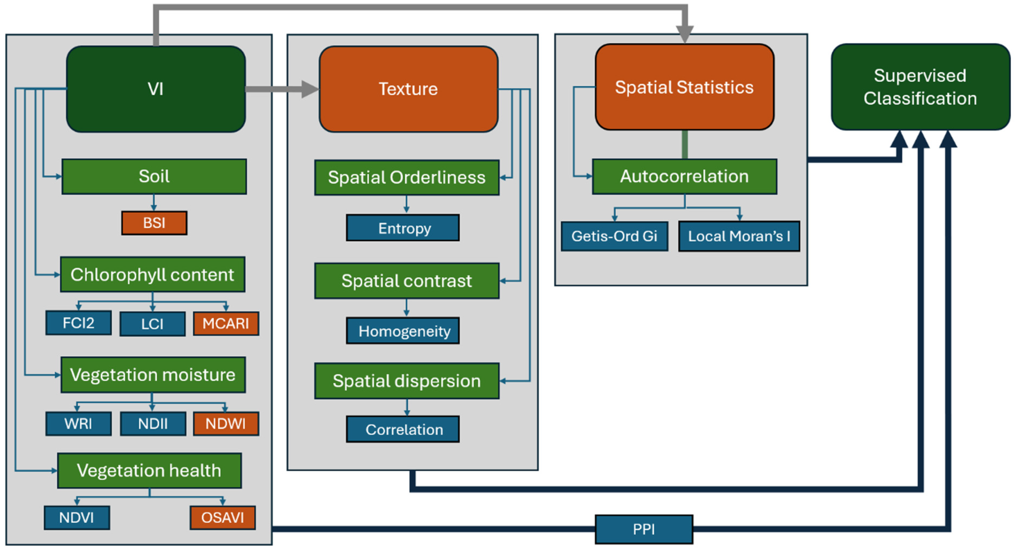
To improve the accuracy of the supervised classification for forest density detection, a set of texture parameters and spatial clustering statistics was calculated in addition to the VIs (Table 2). Specifically, for each VI selected as representative of its respective sub-category (orange-colored indices in Figure 2), three texture parameters were computed. Furthermore, two spatial statistical measures were derived from the same selected indices to capture spatial autocorrelation and clustering patterns.
Finally, the contribution of the Pixel Purity Index (PPI) to classification accuracy was examined [46,47]. The PPI helps identify spectrally pure pixels—such as vegetation, soil, water, or man-made surfaces—using a spectral unmixing approach [48,49,50]. This information provides a useful reference for improving class separability during the classification process.
Specifically, three texture parameters—homogeneity, correlation, and entropy—were calculated for the OSAVI, BSI, MCARI, and NDWI (Figure 2) [51,52]. These four VIs were selected as the most representative of their respective groups because they capture distinct spectral characteristics of vegetation (Table 2) and are largely statistically independent based on their pairwise correlation coefficients (Table 3). Homogeneity was chosen to represent the spatial uniformity of surface features, entropy to describe spatial order or disorder, and correlation to quantify the spatial statistical relationship of neighboring pixels [53]. In addition, two spatial autocorrelation metrics—Local Moran’s I and Getis-Ord Gi—were calculated for the same VIs to assess spatial clustering patterns [54]. Spatial autocorrelation metrics such as Local Moran’s I and Getis-Ord Gi enhance supervised classification by incorporating spatial context. The Local Moran’s I parameter identifies clusters and outliers of similar pixel values, while Getis-Ord Gi detects statistically significant “hot” and “cold” spots. Together, they reduce classification noise and improve class separability, yielding more spatially coherent maps [55,56].
For classification, the Maximum Likelihood algorithm was applied using multiple combinations of input layers derived from the selected parameters. This algorithm was chosen because it is a widely used, robust classification method that generally provides accuracy comparable to more advanced machine-learning approaches such as Support Vector Machines (SVMs) but is computationally faster (e.g., Refs. [57,58]).
Towards this, several studies have shown that, when training samples are sufficient and spectral separability between classes is adequate, the differences in overall accuracy between traditional algorithms such as Maximum Likelihood and machine-learning ones such as SVMs and RF classifiers are often small and may not be practically significant. Moreover, in some cases, the performance differences among classifiers become negligible when the training sample size is large or when classes exhibit distinct spectral signatures [59,60,61,62,63]. Considering the substantially lower computational cost and the satisfactory ROI separability (training samples), the ML classifier was selected as the most efficient and practical approach for the present analysis.
The evaluation of the ML classifier accuracy was tested by calculating two well-known and widely used statistical parameters: the kappa coefficient and the overall accuracy [64,65,66]. Overall accuracy represents the proportion of correctly classified samples relative to the total number of reference (training) samples, providing a general measure of classification performance. The kappa coefficient is a statistical metric that measures the agreement between the classified image and the reference data (training samples), while accounting for agreement occurring by chance, thus providing a more robust evaluation of classification reliability.
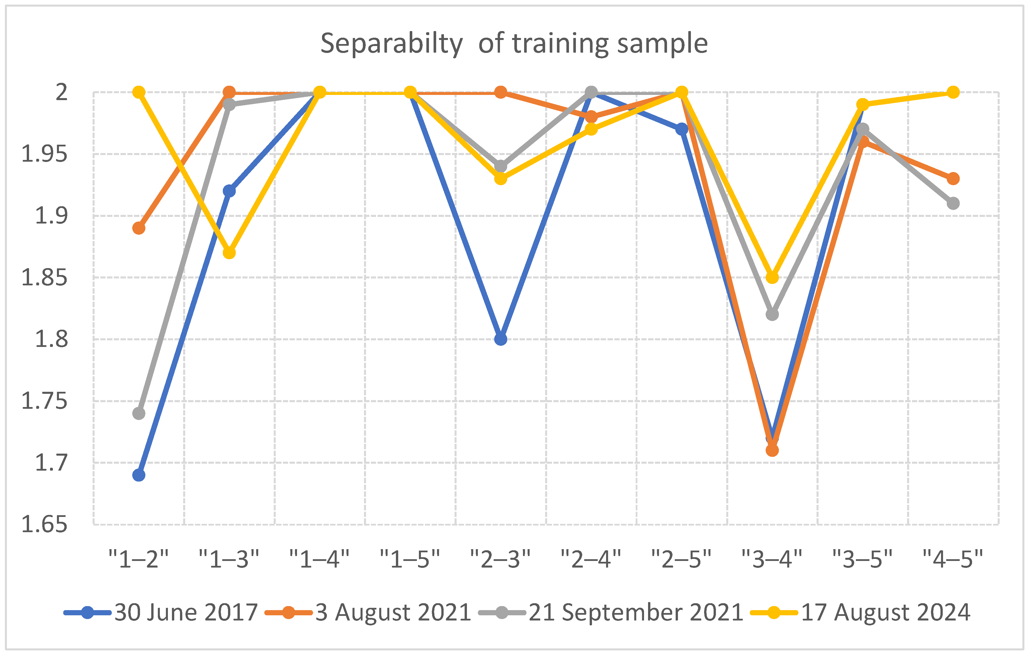
Before applying the Maximum Likelihood classification algorithm with the final set of input layers, the spectral separability of the selected training samples (ROIs) was evaluated. This step serves as an indicator of both the quality of class selection and the degree of spectral independence, which together influence the classification accuracy. Figure 3 presents the separability scores for all class pairs, calculated using the Jeffries–Matusita (JM) metric—a widely used statistical measure in remote sensing image classification [60,61].
The JM distance ranges from 0 to 2.0, where a score of 2.0 indicates perfect separability, and values below 1.7 indicate relatively low separability. As shown in Figure 3, all pairs of the selected classes (corresponding to the training samples) are clearly separable, with JM values above 1.7. For most pairs, scores range between 1.9 and 2.0 across all analyzed images. The lowest separability values were observed between high-density (class 1) and medium-density (class 2) forests, as well as between low-density forest (class 3) and the bare ground (class 4). This result is expected, as these pairs share similar spectral characteristics. Nevertheless, the values remain within acceptable limits, supporting the overall reliability of the classification approach used in this study (Figure 2).

3. Results

Several classification scenarios were established by varying the number and types of input layers, following the general methodological framework shown in Figure 2. For each scenario, the Maximum Likelihood classification algorithm was applied, and post-classification accuracy statistics were computed. Table 4 reports the overall accuracy (expressed as a percentage) and the kappa coefficient (ranging from 0.0 to 1.0) as evaluation metrics for the Maximum Likelihood classification results.
To gain deeper insight into classification accuracy, class-level statistics were derived using a confusion matrix (also known as a contingency matrix). This statistical tool evaluates how many pixels from the reference classes (training samples) were correctly classified and how many were misclassified into other classes by the classification algorithm.
Table 5 presents, for all four multispectral image scenes, the mean percentage of correctly classified pixels for each class, as well as the distribution of misclassified pixels across the other classes.
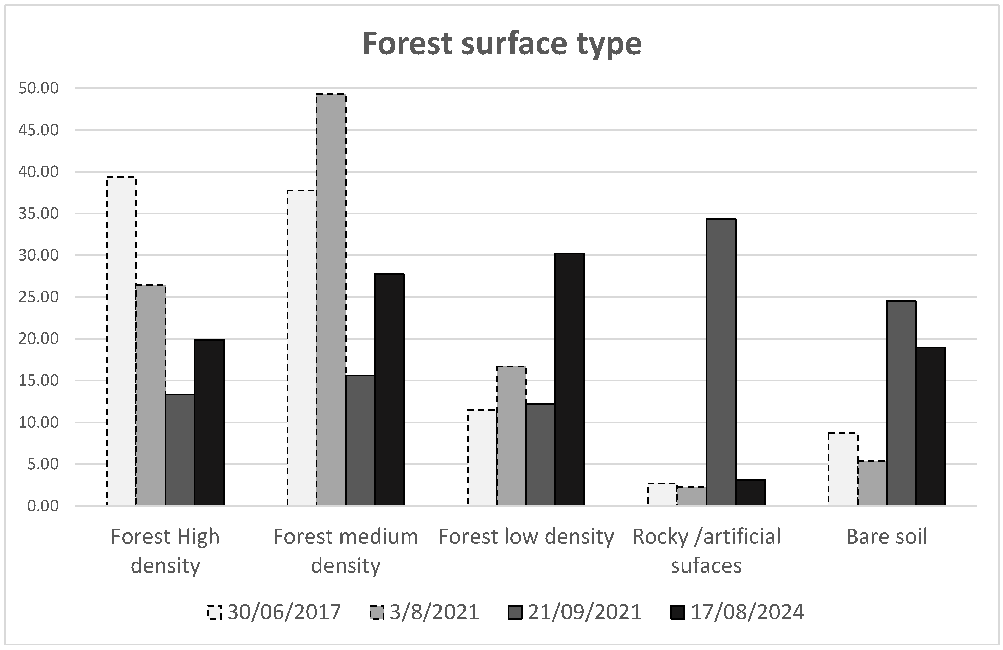
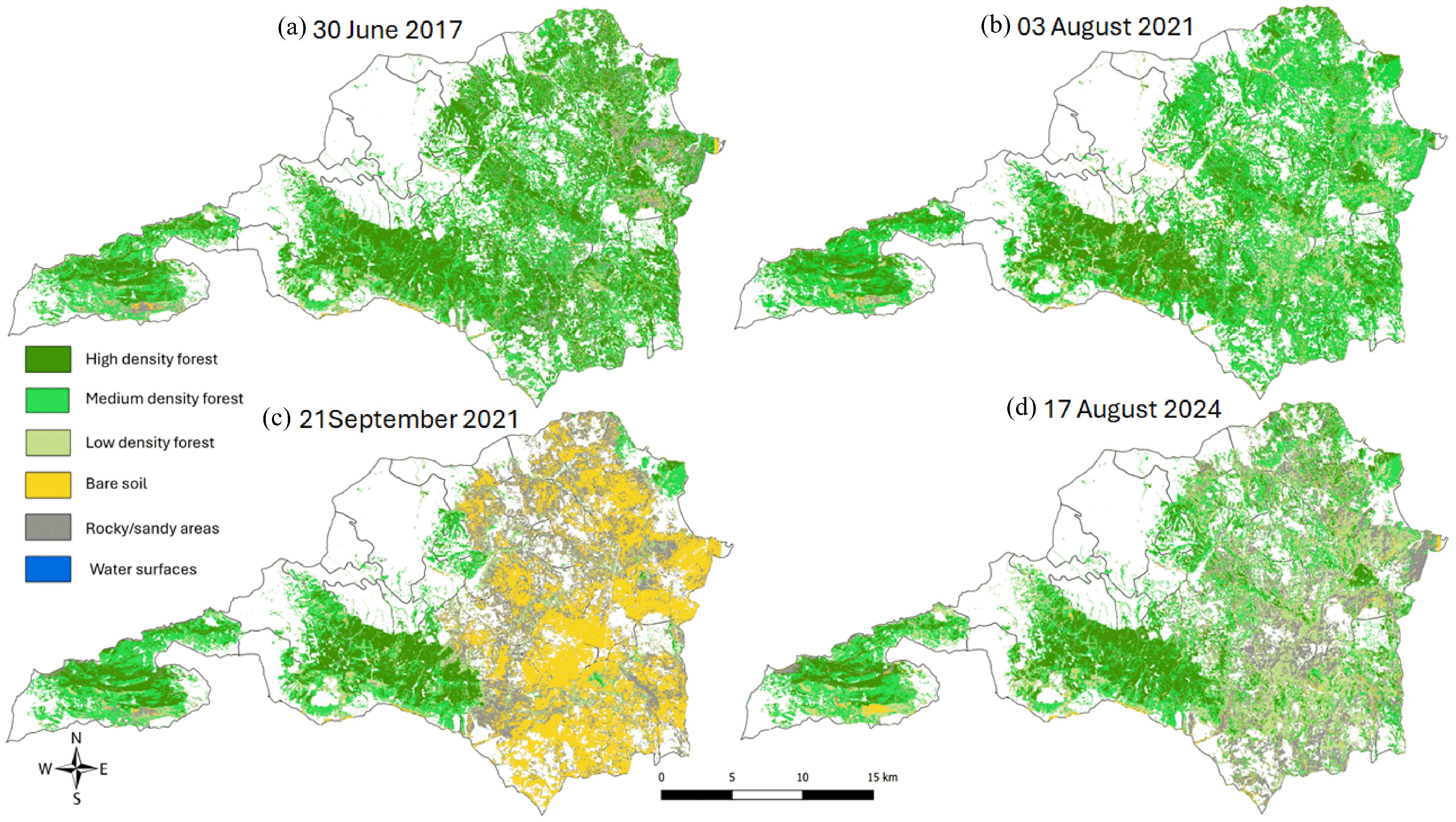
Given the reliability of the classification products, as indicated by the accuracy statistics in Table 4, quantitative assessments of class changes over time were conducted (Figure 4). In Figure 5, the spatial changes in all of the examined classes are presented to depict their distribution in time and space.

4. Discussion

As shown in Table 5, the most spectrally pure and independent classes, based on the selected training samples, are “high-density forest” and “rocky and artificial surfaces.” For these two classes, more than 92% of their pixels remained correctly classified, with very low dispersion into other classes. In contrast, the other classes showed lower spectral purity, with greater dispersion of their pixels into neighboring classes. Notably, 12.05% of pixels labeled as “low-density forest” were classified as “high-density forest” and 16.19% as “medium-density forest.” Similarly, 28.5% of “medium-density forest” training pixels were classified as “high-density forest.” This level of confusion among classes is partly expected, as the forest density classes represent surfaces with very similar land-cover characteristics. Consequently, some degree of spectral overlap—and, therefore, misclassification—is likely, regardless of the classification algorithm used.
A similar pattern was observed between the “bare soil” and “rocky and artificial surface” classes, where mixed surfaces at the pixel level or gradual land-cover transitions resulted in a mean dispersion of 4.69–5.44%. In addition, part of the “bare soil” class was misclassified as “low-density forest,” which is reasonable given that these classes can share partially similar land-cover characteristics (see Table 1).
Overall, misclassification of the training samples was relatively small, ranging from 0.06% to 28.5%, with a mean misclassification rate of 6.3% across all forest density classes. Importantly, a clear distinction was achieved between forest-related classes and non-forest classes. These results indicate that the proposed classification model—comprising the selected input parameters, training samples, and Maximum Likelihood algorithm (Figure 2)—can effectively capture the different forest density levels and associated land-cover classes (e.g., bare soil, rocky surfaces) with high overall accuracy (Table 4).
As shown in Figure 4, the “high-density forest” class exhibited a notable decrease, even between the first two dates (2017 and pre-fire 2021), when no wildfire events occurred. This decrease (approximately 13%) can be attributed to seasonal variations in vegetation canopy moisture between June and August. Because canopy moisture was included as an input parameter through vegetation moisture indices (Figure 2), this factor likely contributed to the observed decline. Part of this change may also be due to classification error, which was approximately 11% for these two dates.
Before the August 2021 wildfire, the mean spatial extent of the “high-density forest” was 32.88% of the study area. After the wildfire, this dropped to 16.63% on average, with the lowest value (13.35%) recorded immediately after the fire. Three years later, the “high-density forest” class showed a significant recovery, increasing to 19.90%.
Similar trends were observed for the “medium-density forest” class. Before the wildfire, this class occupied 43.52% of the forested area, but it declined to 21.68% immediately after the fire. Partial recovery was evident three years later when the class expanded to 27.73% of the forested area.
For the “low-density forest” class, a modest increase (5.24%) was observed during the pre-fire period (Figure 4), likely due to seasonal variations. Immediately after the fire, this class remained relatively stable at 12.19% of the forested area, as much of it was located outside the burn scar. However, three years later, its spatial extent increased dramatically to 30.22%, reflecting natural vegetation regeneration within the burned areas and the transition of land cover into early successional forest.
The “bare soil” class represented an average of 7.05% of the forested area during the pre-fire period. Following the wildfire, its extent increased sharply to 24.51%. This was accompanied by a substantial increase in the “rocky areas” class (from 2.24% to 34.31%). Together, these two classes indicate that nearly 60% of the forested area was affected by the fire. By 2024, a marked decline in both the “bare soil” and “rocky areas” classes was observed, reflecting vegetation regrowth and a shift toward “low-density forest,” indicative of progressive natural reforestation.
The forested area on 30 June 2017 (Figure 5a) has a similar spatial density to the one of 3 August 2021 (Figure 5b). This is expected, because there was no fire event during this period. Notable spatial changes between the two images are observed, primarily in the northern and northeastern parts of the study domain, likely attributable to differences in vegetation moisture conditions.
Just days after the large wildfire of late August 2021, dramatic spatial changes were evident (Figure 5c), with the majority of the forested area within the study domain burned. Three years later, substantial vegetation regeneration was observed; however, forest density remained markedly lower than before the fire. Specifically, many areas classified as “bare soil” or “rocky areas” in September 2021 (Figure 5c) had transitioned primarily into the “low-density forest” class by August 2024 (Figure 5d).
Before the wildfire, forested areas—combining all vegetation density classes—accounted for a mean of 90.48% of the study domain (Figure 1). Immediately after the fire, this dropped to 41.2%, representing a 49.28% loss of vegetation cover. By August 2024, forest cover had partially recovered to 77.85%. Despite this recovery, there remains a net loss of 12.15% of the pre-fire forest area, equivalent to approximately 46.42 km2, which did not regenerate even as low-density vegetation.
Notably, substantial portions of the forested area were converted to the “rocky areas” class, particularly in the central and southeastern parts of the study domain. These areas are likely to be difficult—or even impossible—to reforest under current conditions. Thus, while significant vegetation regeneration has occurred, the results also point to a notable, and potentially permanent, degradation of total forest cover in the region (Figure 5d).

5. Conclusions

This study presents a comprehensive approach for detecting and classifying forest canopy density exclusively using Sentinel-2 multispectral imagery. By exploiting the high spatial and spectral resolution of Sentinel-2, a suite of VIs, texture parameters, and spatial statistics—including PPI, Moran’s I, and Getis-Ord statistics—were derived and evaluated. These parameters were organized into different scenarios in order to investigate their sensitivity and contribution to classification performance. Carefully selected training samples representing the different forest density classes and associated land-cover types were then used in a supervised classification framework implemented with the ML algorithm.
The results demonstrate that the selection and combination of input variables play a critical role in classification performance. When appropriate groups of VIs, texture features, and spatial metrics are employed—ensuring sufficient class separability and complementary physical information—highly accurate forest density maps can be produced. In the optimal scenario tested in this study, the classification achieved an overall accuracy close to 90%. These findings highlight that the quality and diversity of the input parameters may have a stronger influence on classification accuracy than the specific choice of classification algorithm.
An important methodological outcome of this work is that a traditional classifier such as the Maximum Likelihood can produce results comparable to those of more sophisticated machine-learning algorithms, provided that the input feature space is well designed and the training samples exhibit high spectral separability. In addition to achieving competitive accuracy, the ML classifier proved to be significantly faster and more computationally efficient compared with algorithms such as Support Vector Machines (SVMs), which require substantially greater processing time and computational resources. Therefore, the proposed approach offers a practical and cost-effective alternative for large-scale forest monitoring applications.
Another important contribution of this study is the demonstration that forest density can be effectively assessed using only optical multispectral data and their derived indices and spatial metrics without requiring the integration of Synthetic Aperture Radar (SAR) imagery. While SAR data can provide valuable structural information, their use often involves complex preprocessing steps and specialized data handling. The results of this study indicate that carefully selected Sentinel-2-derived spectral and spatial features can provide sufficient information to characterize forest canopy density with high reliability.
Applying the proposed methodology to the pilot study area in northern Euboea provided valuable insights into forest dynamics before and after the catastrophic wildfire of August 2021. Prior to the fire, high-density forest covered approximately 32.9% of the study area, while total forest cover (including all density classes) reached nearly 90%. Bare soil and rocky surfaces accounted for the remaining 10%. Following the wildfire, forest cover declined dramatically, with nearly 49.3% of forested land converted to non-forest classes. Although partial recovery was observed three years later, with forest cover reaching 77.85%, much of the regeneration occurred within the low-density forest class, which is expected given the relatively short post-fire recovery period. The recovery also may be owed to seasonal changes in low vegetation and not reforestation. The long-term forest condition needs continuous monitoring and in situ measurements. Approximately 12.15% of the pre-fire forest area appears to have been lost during the examined period. These results highlight the substantial degradation of the forest structure and spatial extent, with potential long-term implications for ecosystem services, local livelihoods (e.g., ecotourism and forest products), and regional environmental conditions, including surface temperature regulation, soil moisture retention, and water resources.
Overall, the proposed framework demonstrates that Sentinel-2 imagery, combined with carefully selected spectral indices and spatial metrics, can provide a robust and computationally efficient tool for mapping forest canopy density and assessing post-disturbance forest dynamics. Future work will explore the integration of additional data sources, such as SAR observations, to evaluate whether further improvements in classification accuracy can be achieved. Further research will also investigate long-term forest regeneration dynamics and density transitions, particularly in relation to spatiotemporal variations in climatic conditions and disturbance regimes in the region.

Author Contributions

Conceptualization, S.K.; methodology, S.K.; software, S.K. and M.M.; validation, S.K. and M.M.; formal analysis, S.K.; investigation, S.K. and M.M.; resources, M.M.; data curation, M.M.; writing—original draft preparation, M.M.; writing—review and editing, S.K.; visualization, S.K. and M.M.; supervision, S.K. All authors have read and agreed to the published version of the manuscript.

Funding

This research received no external funding. The APC was funded by MDPI Publishing as feature paper.

Data Availability Statement

Research data are not shared.

Acknowledgments

The author acknowledges the providers of all the different datasets used in this study: ESA (European Space Agency) for the free provision of the Sentinel-2 multispectral satellite images through its official portals/services. Also, the author acknowledges the Greek Ministry of Environment for the free access to the forest maps across Greece.

Conflicts of Interest

The authors declare no conflict of interest.

References

  1. Seidl, R.; Thom, D.; Kautz, M.; Martin-Benito, D.; Peltoniemi, M.; Vacchiano, G.; Wild, J.; Ascoli, D.; Petr, M.; Honkaniemi, J.; et al. Forest disturbances under climate change. Nat. Clim. Change 2017, 7, 395–402. [Google Scholar] [CrossRef] [Scilit]
  2. IPCC. Climate Change: Impacts, Adaptation, and Vulnerability. Contribution of Working Group II to the Sixth Assessment Report of the Intergovernmental Panel on Climate Change (IPCC). 2022. Available online: https://www.ipcc.ch/report/ar6/wg2/chapter/chapter-4 (accessed on 4 April 2022).
  3. Dudney, J.; Edwards, J.; Harvey, P.J.; Seidl, R. Climate change effects on interacting disturbances in forests. Annu. Rev. Ecol. Evol. Syst. 2025, 56, 393–420. [Google Scholar] [CrossRef] [Scilit]
  4. Teodoro, A.C.; Duarte, L. The synergy of remote sensing and geographical information systems in the management of natural disasters. In Nanotechnology-Based Smart Remote Sensing Networks for Disaster Prevention; Denizli, A., Alencar, M.S., Nguyen, T.A., Motaung, D.E., Eds.; Elsevier: Amsterdam, The Netherlands, 2018; pp. 303–323. [Google Scholar] [CrossRef] [Scilit]
  5. Hansen, M.C.; Potapov, P.V.; Moore, R.; Hancher, M.; Turubanova, S.A.; Tyukavina, A.; Thau, D.; Stehman, S.V.; Goetz, S.J.; Loveland, T.R.; et al. High-resolution global maps of 21st-century forest cover change. Science 2013, 342, 850–853. [Google Scholar] [CrossRef] [Scilit] [PubMed]
  6. Wang, Y.; Sun, Y.; Cao, X.; Wang, Y.; Zhang, W.; Cheng, X. A review of regional and global scale land use/land cover mapping products generated from satellite remote sensing. ISPRS J. Photogramm. Remote Sens. 2023, 206, 311–334. [Google Scholar] [CrossRef] [Scilit]
  7. Jing, Q.; He, J.; Li, Y.; Yang, X.; Peng, Y.; Wang, H.; Yu, F.; Wu, J.; Gong, S.; Che, H.; et al. Analysis of the spatiotemporal changes in global land use from 2001 to 2020. Sci. Total Environ. 2024, 908, 168354. [Google Scholar] [CrossRef] [Scilit]
  8. Li, L.; Awada, T.; Zhang, Y.; Paustian, K. Global land use change and its impact on greenhouse gas emissions. Glob. Change Biol. 2024, 30, e17604. [Google Scholar] [CrossRef] [Scilit] [PubMed]
  9. Chen, M.; Samat, N.; Tilaki, M.J.M.; Duan, L. Land use/cover change simulation research: A systematic review and bibliometric analysis. Ecol. Indic. 2025, 170, 112991. [Google Scholar] [CrossRef] [Scilit]
  10. Cunningham, C.X.; Williamson, G.J.; Bowman, S. Increasing frequency and intensity of the most extreme wildfires on Earth. Nat. Ecol. Evol. 2024, 8, 1420–1425. [Google Scholar] [CrossRef] [Scilit]
  11. Law, B.E.; Abatzoglou, J.; Schwalm, C.; Byrne, D.; Fann, N.; Nassikas, N.J. Anthropogenic climate change contributes to wildfire-driven air pollution and extreme fire years. Commun. Earth Environ. 2025, 6, 336. [Google Scholar] [CrossRef] [Scilit]
  12. Wasserman, T.N.; Mueller, S. Climate influences on future fire severity: A synthesis of regional trends and projections. Fire Ecol. 2023, 19, 2. [Google Scholar] [CrossRef] [Scilit]
  13. Senande-Rivera, M.; Insua-Costa, D.; Miguez-Macho, G. Spatial and temporal expansion of global wildland fire risk under climate change. Nat. Commun. 2022, 13, 28835. [Google Scholar] [CrossRef] [Scilit] [PubMed]
  14. Yousefpour, R.; Gray, D.R. Managing Forest risks in uncertain times of climate change necessitates novel, adaptive forest decision approaches. Ann. For. Sci. 2022, 79, 16. [Google Scholar] [CrossRef] [Scilit]
  15. Davis, K.T.; Peeler, J.; Fargione, J.; Huago, R.D.; Metlen, K.; Robles, M.D.; Woolley, T. Tamm review: A meta-analysis of thinning, prescribed fire, and wildfire effects on subsequent wildfire severity in conifer dominated forests of the Western US. For. Ecol. Manag. 2024, 561, 121885. [Google Scholar] [CrossRef] [Scilit]
  16. Zhang, M.; Yu, S.; Ye, Q.; Li, Z.; Yin, D.; Zhao, Z. Effect of the Grain-for-Green Program on forest fragmentation and forest cover changes. Land Degrad. Dev. 2023, 34, 3208–3224. [Google Scholar] [CrossRef] [Scilit]
  17. Phiri, D.; Simwanda, M.; Salekin, S.; Nyirenda, V.; Murayama, Y.; Ranagalage, M. Sentinel-2 data for land cover/use mapping: A review. Remote Sens. 2020, 12, 2291. [Google Scholar] [CrossRef] [Scilit]
  18. Pandey, P.C.; Koutsias, N.; Petropoulos, G.P.; Srivastava, P.K.; Ben Dor, E. Land use/land cover in view of earth observation: Data sources, input dimensions, and classifiers—A review of the state of the art. Geocarto Int. 2019, 36, 957–988. [Google Scholar] [CrossRef] [Scilit]
  19. Hu, X.; Li, L.; Huang, J.; Zeng, Y.; Zhang, S.; Su, Y.; Hong, Y.; Hong, Z. Radar vegetation indices for monitoring surface vegetation: Development, challenges and trends. Sci. Total Environ. 2024, 945, 173974. [Google Scholar] [CrossRef] [Scilit]
  20. Aranguren, I.; González-Audícana, M.; Montero, E.; Sanz, J.A.; Álvarez-Mozos, J. Assessing the synergistic use of Sentinel-1, Sentinel-2, and LiDAR data for forest type and species classification. Remote Sens. 2025, 17, 2028. [Google Scholar] [CrossRef] [Scilit]
  21. Gautam, A.; Narine, L.L.; Anderson, C.J.; Cristan, R. Synergistic use of ICESat-2 LiDAR and Sentinel-2 imagery for forest structural monitoring. Environ. Monit. Assess. 2025, 197, 183. [Google Scholar] [CrossRef] [Scilit]
  22. Lawrence, B.L. Modeling stand-level forest attributes using lidar and common stand exam data. Remote Sens. Appl. Soc. Environ. 2025, 40, 101794. [Google Scholar] [CrossRef] [Scilit]
  23. Le, T.S.; Harper, R.; Dell, B. Application of remote sensing in detecting and monitoring water stress in forests. Remote Sens. 2023, 15, 3360. [Google Scholar] [CrossRef] [Scilit]
  24. Wulder, M.A.; Loveland, T.; Roy, D.; Crawford, C.J.; Masek, J.G.; Woodcock, C.E.; Allen, R.G.; Anderson, M.C.; Belward, A.S.; Cohen, W.B.; et al. Current status of Landsat program, science, and applications. Remote Sens. Environ. 2023, 4, 3–21. [Google Scholar] [CrossRef] [Scilit]
  25. Santoro, M.; Cartus, O. ESA Biomass Climate Change Initiative (Biomass_cci): Global Datasets of Forest Above-Ground Biomass for the Years 2010, 2017, 2018, 2019 and 2020, v4; NERC EDS Centre for Environmental Data Analysis: Didcot, UK, 2023. [CrossRef]
  26. Torres, R.; Snoeij, P.; Geudtner, D.; Bibby, D.; Davidson, M.; Attema, E.; Potin, P.; Rommen, B.; Floury, N.; Brown, M.; et al. GMES Sentinel-1 mission. Remote Sens. Environ. 2012, 120, 9–24. [Google Scholar] [CrossRef] [Scilit]
  27. Gao, Y.; Solórzano, J.V.; Skutsch, M.; Cao, Y.; Estoque, R.C.; Szantoi, Z.; Taud, H. Estimating forest degradation by capturing temporal change in biomass density: Insights from a tropical dry forest. Remote Sens. Appl. Soc. Environ. 2025, 40, 101775. [Google Scholar] [CrossRef] [Scilit]
  28. Rikimaru, A.; Roy, P.S.; Miyatake, S. Tropical forest cover density mapping. Trop. Ecol. 2002, 43, 39–47. [Google Scholar]
  29. Kwon, T.H.; Lee, W.K.; Kwak, D.A.; Park, T.J.; Lee, J.Y.; Hong, S.Y.; Guishan, C.; Kim, S.-R. Forest canopy density estimation using airborne hyperspectral data. Korean J. Remote Sens. 2012, 28, 297–309. [Google Scholar] [CrossRef] [Scilit]
  30. Das, S.; Ghosh, D.; Sarkar, A.; Chatterjee, U.; Mandal, S.; Malo, S.K.; Rahaman, S.; Das, M.; Saha, S.; Chouhan, P. Prediction of deforestation risk in north-east India: Evaluating forest canopy density dynamics and spatial drivers through machine learning models. Environ. Sci. 2025, 37, 194. [Google Scholar] [CrossRef] [Scilit]
  31. Drusch, M.; Del Bello, U.; Carlier, S.; Colin, O.; Fernandez, V.; Gascon, F.; Hoersch, B.; Isola, C.; Laberinti, P.; Martimort, P.; et al. Sentinel-2: ESA’s optical high-resolution mission for GMES operational services. Remote Sens. Environ. 2012, 120, 25–36. [Google Scholar] [CrossRef] [Scilit]
  32. Immitzer, M.; Vuolo, F.; Atzberger, C. First experience with Sentinel-2 data for crop and tree species classifications in central Europe. Remote Sens. 2016, 8, 166. [Google Scholar] [CrossRef] [Scilit]
  33. Kumari, A.; Karthikeyan, S. Sentinel-2 Data for Land Use/Land Cover Mapping: A Meta-analysis and Review. Comput. Sci. 2023, 4, 815. [Google Scholar] [CrossRef] [Scilit]
  34. López-García, J.; Manzo-Delgado, L.M.; Cruz-Bello, G.M.; Torres-González, M.A. Integrating visual interpretation and forest canopy density modeling to monitor forest canopy density in Central Mexico. Model. Earth Syst. Environ. 2026, 12, 38. [Google Scholar] [CrossRef] [Scilit]
  35. Rouse, J.; Haas, R.; Schell, J.; Deering, D. Monitoring vegetation systems in the Great Plains with ERTS. In Third ERTS Symposium NASA; Remote Sensing Center, Texas A&M University: College Station, TX, USA, 1973; pp. 309–317. [Google Scholar]
  36. Rondeaux, G.; Steven, M.; Baret, F. Optimization of soil-adjusted vegetation indices. Remote Sens. Environ. 1996, 55, 95–107. [Google Scholar] [CrossRef] [Scilit]
  37. Datt, B. Remote sensing of water content in Eucalyptus leaves. J. Plant Physiol. 1999, 154, 30–36. [Google Scholar] [CrossRef] [Scilit]
  38. Becker, S.J.; Daughtry, C.S.T.; Russ, A.L. Robust forest cover indices for multispectral images. Photogramm. Eng. Remote Sens. 2018, 84, 505–512. [Google Scholar] [CrossRef] [Scilit]
  39. Daughtry, C.; Walthall, C.L.; Kim, M.S.; De Colstoun, E.B.; McMurtrey, J.E. Estimating corn leaf chlorophyll concentration from leaf and canopy reflectance. Remote Sens. Environ. 2000, 74, 229–239. [Google Scholar] [CrossRef] [Scilit]
  40. Gong, A.; Huang, Z.; Liu, L.; Yang, Y.; Ba, W.; Wang, H. Development of an index for forest fire risk assessment considering hazard factors and the hazard-formative environment. Remote Sens. 2023, 15, 5077. [Google Scholar] [CrossRef] [Scilit]
  41. Zhao, H.; Chen, X.; Area, A.S. Use of normalized difference bareness index in quickly mapping bare areas from ETM/ETM+. In International Geoscience and Remote Sensing Symposium; IEEE: New York, NY, USA, 2005; Volume 3, p. 1666. [Google Scholar] [CrossRef] [Scilit]
  42. Shen, L.; Li, C. Water body extraction from Landsat ETM+ imagery using AdaBoost algorithm. In Proceedings of the 18th International Conference on Geoinformatics 2010, Beijing, China, 18–20 June 2010; pp. 1–4. [Google Scholar]
  43. McFeeters, S.K. The use of the normalized difference water index (NDWI) in the delineation of open water features. Int. J. Remote Sens. 1996, 17, 1425–1432. [Google Scholar] [CrossRef] [Scilit]
  44. Xu, H. Modification of normalized difference water index (NDWI) to enhance open water features in remotely sensed imagery. Int. J. Remote Sens. 2006, 27, 3025–3033. [Google Scholar] [CrossRef] [Scilit]
  45. Hardisky, M.; Klemas, V.; Smart, R. Influences of soil salinity, growth form, and leaf moisture on spectral reflectance of Spartina alterniflora canopies. Photogramm. Eng. Remote Sens. 1983, 49, 77–83. [Google Scholar]
  46. Chang, C.-I.; Wu, C.-C. Iterative Pixel Purity Index. In Proceedings of the 4th Workshop on Hyperspectral Image and Signal Processing: Evolution in Remote Sensing (WHISPERS), Shanghai, China, 4 June 2012; pp. 1–4. [Google Scholar] [CrossRef] [Scilit]
  47. Plaza, A.; Chang, C.-I. Fast implementation of pixel purity index algorithm. In Proceedings of the Algorithms and Technologies for Multispectral, Hyperspectral, and Ultraspectral Imagery XI; Proceedings of SPIE; SPIE (The International Society for Optical Engineering): Bellingham, WA, USA, 2005; Volume 5806. [Google Scholar] [CrossRef] [Scilit]
  48. Boardman, J.W.; Kruse, F.A.; Green, R.O. Mapping target signatures via partial unmixing of AVIRIS data. In Summaries of the Fifth Annual JPL Airborne Earth Science Workshop; NASA Jet Propulsion Laboratory: Pasadena, CA, USA, 1995; pp. 23–26. Available online: https://ntrs.nasa.gov/citations/19950027316 (accessed on 24 March 2026).
  49. Clark, R.N.; Swayze, G.A.; Livo, K.E.; Kokaly, R.; Sutley, S.; Dalton, B.; McDougal, R.; Gent, C. Imaging spectroscopy: Earth and Planetary remote sensing with the USGS Tetracorder and expert systems. J. Geophys. Res. Anal. 2003, 108, 5131. [Google Scholar] [CrossRef] [Scilit]
  50. Keshava, N.; Mustard, J.F. Spectral unmixing. IEEE Signal Process. Mag. 2002, 19, 44–57. [Google Scholar] [CrossRef] [Scilit]
  51. Puissant, A.; Hirsch, J.; Weber, C. Utility of texture analysis to improve per-pixel classification for very high spatial resolution imagery. Int. J. Remote Sens. 2006, 26, 733–745. [Google Scholar] [CrossRef] [Scilit]
  52. Mohammadpour, P.; Viegas, D.; Viegas, C. Vegetation mapping with random forest using Sentinel-2 and GLCM texture features: A case study of the Lousã region, Portugal. Remote Sens. 2022, 14, 4585. [Google Scholar] [CrossRef] [Scilit]
  53. Gu, J.; Chen, J.; Zhou, Q.M.; Zhang, H.W.; Ma, L. Quantitative textural parameter selection for residential extraction from high-resolution imagery. Int. Arch. Photogramm. Remote Sens. Spatial Inf. Sci. 2008, 37. Available online: https://www.isprs.org/proceedings/xxxvii/congress/4_pdf/241.pdf (accessed on 24 March 2026).
  54. Rey, S.; Arribas-Bel, D.; Wolf, L. Geographic Data Science with Python; Chapman & Hall/CRC Press: Boca Raton, FL, USA, 2023. [Google Scholar]
  55. Anselin, L. Local indicators of spatial association—LISA. Geogr. Anal. 1995, 27, 93–115. [Google Scholar] [CrossRef] [Scilit]
  56. Getis, A.; Ord, J.K. Analysis of spatial association by use of distance statistics. Geogr. Anal. 1992, 24, 189–206. [Google Scholar] [CrossRef] [Scilit]
  57. Szuster, B.W.; Chen, Q.; Borger, M. Comparison of classification techniques for land-use analysis in tropical coastal zones. Appl. Geogr. 2011, 31, 525–532. [Google Scholar] [CrossRef] [Scilit]
  58. Aziz, N.A. Accuracy comparison of supervised classification methods using Sentinel-2 imagery in the Al-Hawizeh Marsh Area, Southern Iraq. Geomat. Environ. Eng. 2021, 15, 5–21. [Google Scholar] [CrossRef] [Scilit]
  59. Chowdhury, M.S. Comparison of accuracy and reliability of random forest, support vector machine, and maximum likelihood method in land use/land cover classification of urban setting. Geosci. Chall. 2023, 14, 100800. [Google Scholar] [CrossRef] [Scilit]
  60. Padma, S.; Sanjeevi, S. Jeffries–Matusita based mixed-measure for improved spectral matching in hyperspectral imagery. Int. J. Appl. Earth Obs. Geoinf. 2014, 32, 138–151. [Google Scholar] [CrossRef] [Scilit]
  61. Wicaksono, P.; Aryaguna, P.A. Inter-class spectral separability and classification accuracy of benthic habitat mapping. Remote Sens. Appl. Soc. Environ. 2020, 19, 100335. [Google Scholar] [CrossRef] [Scilit]
  62. Noi, P.T.; Kappas, M. Comparison of random forest, k-nearest neighbor, and support vector machine classifiers for land cover classification using Sentinel-2 imagery. Sensors 2018, 18, 18. [Google Scholar] [CrossRef] [Scilit]
  63. Otukei, J.R.; Blaschke, T. Land cover change assessment using decision trees, support vector machines and maximum likelihood classification algorithms. Int. J. Appl. Earth Obs. Geoinf. 2010, 12, S27–S31. [Google Scholar] [CrossRef] [Scilit]
  64. Congalton, R.G. A review assessing the accuracy of classifications of remotely sensed data. Remote Sens. Environ. 1991, 37, 35–46. [Google Scholar] [CrossRef] [Scilit]
  65. Foody, G.M. Status of land cover classification accuracy assessment. Remote Sens. Environ. 2002, 80, 185–201. [Google Scholar] [CrossRef] [Scilit]
  66. Kvålseth, T.O. Kappa Coefficient of Agreement. In International Encyclopedia of Statistical Science; Lovric, M., Ed.; Springer: Berlin/Heidelberg, Germany, 2025. [Google Scholar] [CrossRef] [Scilit]
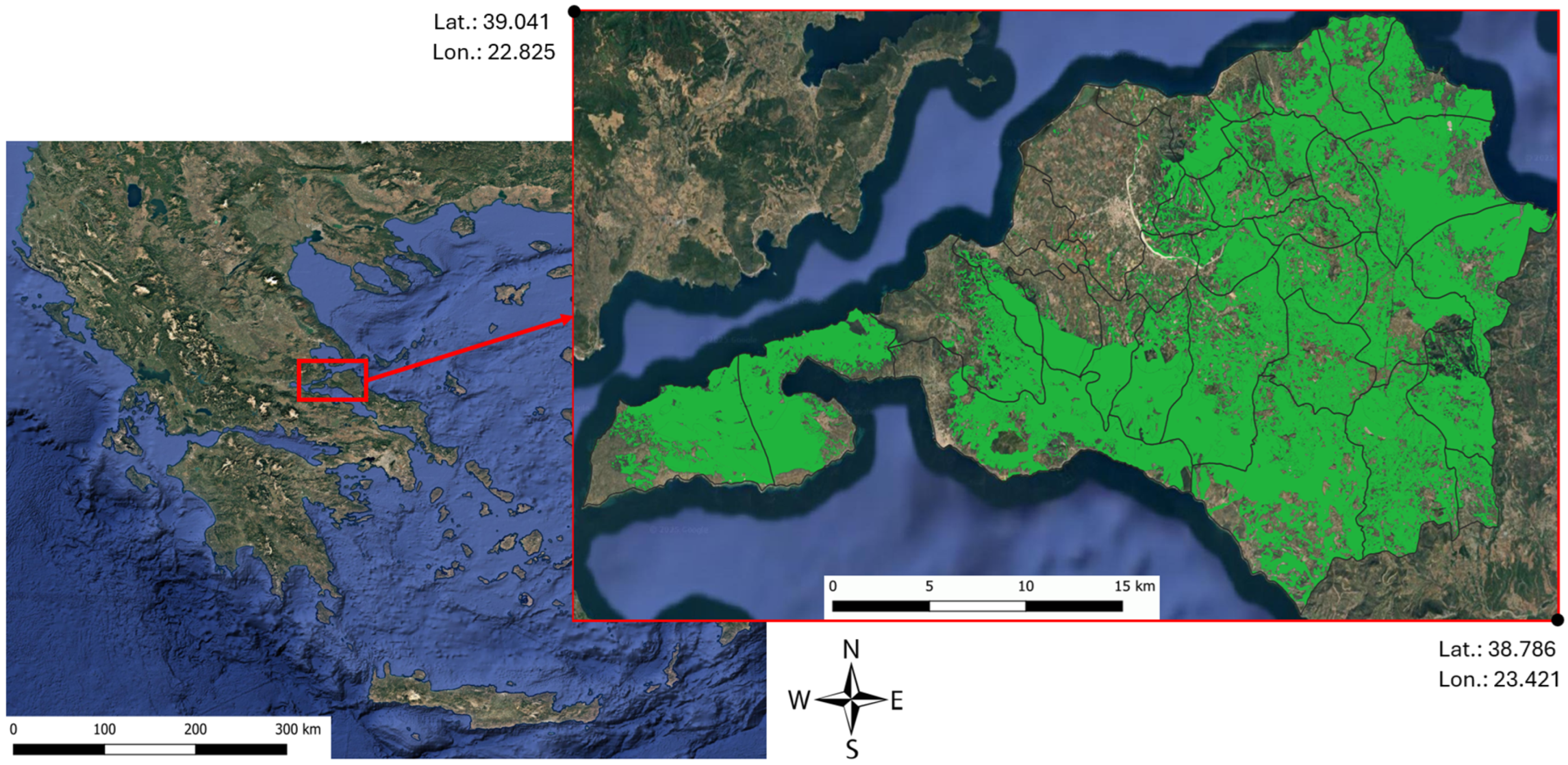
Figure 1. The study domain (Greek peninsula) on the left, focusing on the forested area (green colored) of the northern part of the Euboea Island (Aegean Sea) on the right. The black polygons represent local administrative boundaries of the region, and the geographical limits are provided in decimal degrees (WGS 84 Projection System).
Geomatics 06 00033 g001
Figure 2. General model scheme for the groups of input data layers that were used in the supervised classification procedure about the forest density of the study domain.
Geomatics 06 00033 g002
Figure 3. Spectral separability of the different pairs of training samples according to “Jeffries–Matusita” metric. The label “1” is the high-density forest class, label “2” is the medium-density forest class, label “3” is the low-density forest class, label “4” is the bare soil class, while label “5” is the rocky/artificial surface class.
Geomatics 06 00033 g003
Figure 4. The percentage of the different land-cover types inside the forested area of the study domain for all the selected dates.
Geomatics 06 00033 g004
Figure 5. Forest density classes of the study domain and all the others (a) on 30 June 2017, (b) 3 August 2021, (c) 21 September 2021 and (d) 17 August 2024.
Geomatics 06 00033 g005
Table 1. Image examples of the image samples that were selected for each of the classes of interest used.
Class
(Number of Pixels)
Indicative SampleDescription
Dense forest (2046)Geomatics 06 00033 i001Dense forest canopy.
Medium-density forest (1285)Geomatics 06 00033 i002Medium forest density where among small gaps of the tree canopy, land surface occurs.
Low-density forest
(1319)
Geomatics 06 00033 i003Sparse forest density, frequently mixed with grassland.
Bare soil (1382)Geomatics 06 00033 i004Bare ground with little or no vegetation.
Rocky areas, etc. (992)Geomatics 06 00033 i005Rocky ground surface with little or no vegetation.
Table 2. The remote sensing indices used in the study. The subscript number of the equations underlines the wavelength in nanometers (nm). These indices calculated for the closest spectral bands of the Sentinel-2 multispectral imagery (B2: 490 nm, B3: 560 nm; B4: 665 nm, B5: 705 nm; B8: 842 nm B8A: 865 nm; and B11 = 1610 nm).
Index Category (Groups)FormulaShort Description
healthy vegetation N D V I = ( r 842 r 665 )   ( r 842 + r 665 ) NDVI (Normalized Difference Vegetation Index): This index is a measure of healthy, green vegetation. The combination of its normalized difference formulation and use of the highest absorption and reflectance regions of chlorophyll make it robust over a wide range of conditions [35].
O S A V I = ( r 842 r 665 )   ( r 842 + r 665 + 0.16 ) OSAVI (Optimized Soil Adjusted Vegetation Index): It uses a standard value of 0.16 for the canopy background adjustment factor. This value is considered to be what provides greater soil variation than SAVI for low vegetation cover, while demonstrating increased sensitivity to vegetation cover greater than 50% [36].
chlorophyll content in higher plants L C I = ( r 865 r 705 )   ( r 865 + r 665 ) LCI (Leaf Chlorophyll Index): This index is used to estimate chlorophyll content in higher plants sensitive to variation in reflectance caused by chlorophyll absorption [37].
F C I 2 = r 665 x     r 842 FCI2 (Forest Cover Index): This index distinguishes forest canopies from other types of vegetation using multispectral reflectance imagery that does not include a red edge band [38].
M C A R I = [ ( r 705 r 665 ) 0.2 x   ( r 705 r 560 ) ] x   ( r 705   r 665 ) MCARI (Modified Chlorophyll Absorption Ratio Index): This index indicates the relative abundance of chlorophyll [39].
bare soil B S I = r 1610 + r 842 ( r 842 + r 490 ) r 1610 + r 842 + ( r 842 + r 490 ) BSI (Bare Soil Index): This index is designed to distinguish bare surfaces from vegetated or water-covered areas, making it valuable for land degradation, erosion, and land-cover studies [40,41].
moisture in vegetation W R I = ( r 560 + r 665 )   ( r 842 + r 1610 ) WRI (Water Ratio Index): This index can be used to determine the amount of moisture in vegetation. The calculation technique of this index is based on the ratio between the full spectral index of two visible light ranges (green and red) and shortwave and mid-wave infrared ranges [42].
N W D I = r 560 r 842 ( r 560 + r 842 ) NDWI (Normalized Difference Water Index): This index is sensitive to changes in vegetation canopy water content because it uses the reflectance in the green band while minimizing land and vegetation reflectance using the near-infrared (NIR) band. It is commonly used for water body extraction and flood monitoring [43,44].
N D I I = ( r 842 r 665 )   ( r 842 + r 665 ) NDII (Normalized Difference Infrared Index): This index is a reflectance measurement that is sensitive to changes in water content of plant canopies. The NDII values increase with increasing water content. Applications include crop agricultural management, forest canopy monitoring, and vegetation stress detection [45].
Table 3. Mean correlation coefficients (from all the image scenes) considering all the pixels of the forested areas. The values in bold text refer to the correlation coefficient of the VI finally used.
OSAVINDVILCIFCIBSIWRINDWINDIIMCARI
OSAVI-0.980.160.010.08−0.88−0.890.610.59
NDVI0.98-0.15−0.010.10−0.88−0.880.600.60
LCI0.160.15-0.24−0.12−0.04−0.200.35−0.05
FCI0.01−0.010.24-−0.16−0.01−0.170.17−0.10
BSI0.080.10−0.12−0.16-−0.33−0.07−0.320.10
WRI−0.88−0.88−0.04−0.01−0.33-0.83−0.22−0.57
NDWI−0.89−0.88−0.20−0.17−0.070.83-−0.50−0.34
NDII0.610.600.350.17−0.32−0.22−0.50-0.19
MCARI0.590.60−0.05−0.100.10−0.57−0.340.19-
Table 4. Overall classification accuracy (%) and kappa coefficient (“*”) for the “Maximum Likelihood” classifier, among different parameterization schemes regarding the type and the number of input layers, were used for the classification.
ScenarioDates
17 August 202421 September 20213 August 202130 June 2017
Vegetation Indices85.78
* 0.808
86.86
* 0.826
85.37
* 0.804
84.29
* 0.788
Vegetation Indices &
Pixel Purity Index
85.53
* 0.805
86.90
* 0.8260
85.38
* 0.8043
75.46
* 0.6387
Vegetation Indices &
Texture Parameters
87.49
* 0.832
87.60
*0.835
86.49
* 0.820
85.50
* 0.805
Vegetation Indices &
Texture Parameters &
Pixel Purity Index
87.36
* 0.8301
87.90
* 0.8393
86.74
* 0.823
85.43
* 0.804
Vegetation Indices &
Spatial parameters
86.84
* 0.823
88.07
* 0.841
87.68
* 0.835
84.78
* 0.795
Vegetation Indices &
Spatial parameters &
Pixel Purity Index
86.89
* 0.8241
88.34
* 0.8449
87.66
* 0.835
84.80
* 0.796
Vegetation Indices &
Texture Parameters &
Spatial parameters
88.94
* 0.852
89.11
* 0.855
88.58
* 0.847
85.99
* 0.812
Vegetation Indices &
Texture Parameters &
Spatial parameters &
Pixel Purity Index
89.1
* 0.853
89.40
* 0.858
88.61
* 0.848
86.01
* 0.812
Table 5. Percentage (%) (mean values of all the examined images) of the pixels of the training sample were correctly classified.
Classification SAMPLESReference Samples
Forest High DensityForest Low DensityForest Medium DensityRocky & Artificial SufacesBare Soil
Forest High density92.36512.052528.50250.97255.855
Forest low density0.507566.39254.5150.552511.925
Forest medium density6.89516.187565.8551.6853.715
Rocky & artificial sufaces0.0750.87250.0692.09755.448
Bare soil0.164.49251.31754.69573.058
Disclaimer/Publisher’s Note: The statements, opinions and data contained in all publications are solely those of the individual author(s) and contributor(s) and not of MDPI and/or the editor(s). MDPI and/or the editor(s) disclaim responsibility for any injury to people or property resulting from any ideas, methods, instructions or products referred to in the content.