Clustering-Based TLS Accuracy Zonation to Support Landslide Survey Design

Abstract

This work presents a simulation-based approach to support the planning of Terrestrial Laser Scanning (TLS) surveys for landslide monitoring. Starting from an approximate digital model of the slope, the method estimates the spatial distribution of positional error induced by scanner characteristics, laser beam divergence and, critically, by the incidence angle between the laser beam and the local surface normal. Because complex morphologies cause rapid local variations in incidence angle, neighbouring points may exhibit markedly different error magnitudes, making a direct classification of raw error values insufficient to delineate homogeneous areas. To address this, a multidimensional variable is defined for each simulated point, combining position, estimated error, distance from the scanner and incidence angle. After dimensionality reduction through PCA, the dataset is clustered using K-means with a sufficiently large number of clusters to preserve spatial resolution. Each cluster is associated with a representative error level, and clusters are then merged into broader error classes that delineate zones of comparable expected precision. The procedure is repeated for alternative scanner positions, enabling a comparative evaluation of achievable accuracy across the slope and the identification of areas requiring multiple scans. The method provides a quantitative, reproducible framework to guide TLS station selection and optimize survey design in complex morphological settings.

1. Introduction

Several techniques of varying complexity and operational effort can be employed for the survey and monitoring of landslide-prone slopes, ranging from ground-based measurements to UAV photogrammetry and LiDAR.

Among these, long-range Terrestrial Laser Scanning (TLS) offers an effective solution due to its rapid data acquisition and high-density 3D point clouds. Multiple scans from different stations allow for a detailed reconstruction of morphologically complex surfaces.

A crucial aspect of efficient TLS surveying is the planning of acquisition campaigns. The choice of station locations strongly influences both the completeness and the accuracy of the slope coverage. In practice, station placement is often determined empirically—based on operator experience and field visibility—without quantitative tools that allow comparison of alternative configurations.

This empirical approach can be effectively complemented by simulations that enable a quantitative evaluation of the expected performance of different TLS configurations, considering both slope visibility and achievable measurement precision.

Virtual laser scanning simulators, such as HELIOS++ [1], allow the assessment of alternative stationing scenarios and the estimation of both coverage and data quality as a function of surface morphology. However, there remains a need for systematic approaches capable of quantitatively assessing positional uncertainty as a function of scanning geometry and surface shape.

The main sources of TLS measurement error [2] depend not only on external factors such as atmosphere, humidity, and surface reflectivity but also on intrinsic instrument precision and beam divergence [3,4]. The beam divergence determines the laser footprint size at different ranges and can be modeled through Gaussian propagation.

TLS instruments emit a collimated laser beam that can be approximated by the fundamental Transverse Electromagnetic Mode (TEM00) characterized by a Gaussian transverse irradiance profile. The irradiance distribution can be expressed as $I\left(r\right)=I_0\mathit{exp}\left(-2r^2/w^2\right)$ where w is the beam radius at the 1/e² intensity level, as specified by manufacturers, $I_0$ is the maximum intensity along the beam axis, and r is the radial distance from the beam center. Once normalized, this expression corresponds to a two-dimensional Gaussian probability density with standard deviation s = w/$\sqrt{2}$.

When the beam intersects an inclined planar facet, the circular 1/e² contour is geometrically projected into an ellipse whose semi-axes depend on the incidence angle and local surface orientation. This provides a physically grounded basis for modelling the footprint as an elliptical Gaussian distribution, consistent with established TLS error models.

Building on this concept, [5] introduced an advanced uncertainty model that treats the laser footprint as an elliptical Gaussian distribution on the TIN facets. By projecting the beam geometry onto each triangular surface element, the method derives the complete three-dimensional variance–covariance matrix of the centroid in the global reference frame, capturing the combined effects of beam divergence, surface orientation, and incidence angle. This provides a physically grounded framework for simulating TLS measurement uncertainty, particularly valuable in rugged terrain.

The interaction between scanning geometry and surface morphology, particularly the dependence of error on range and incidence angle, plays a key role [6,7,8].

In rugged or highly variable terrain, such as active landslides, incidence angles may change abruptly even between neighbouring facets. As a result, simulated positional errors often exhibit sharp local discontinuities, making it difficult to identify homogeneous areas simply through classification of error values.

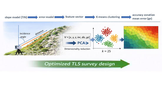
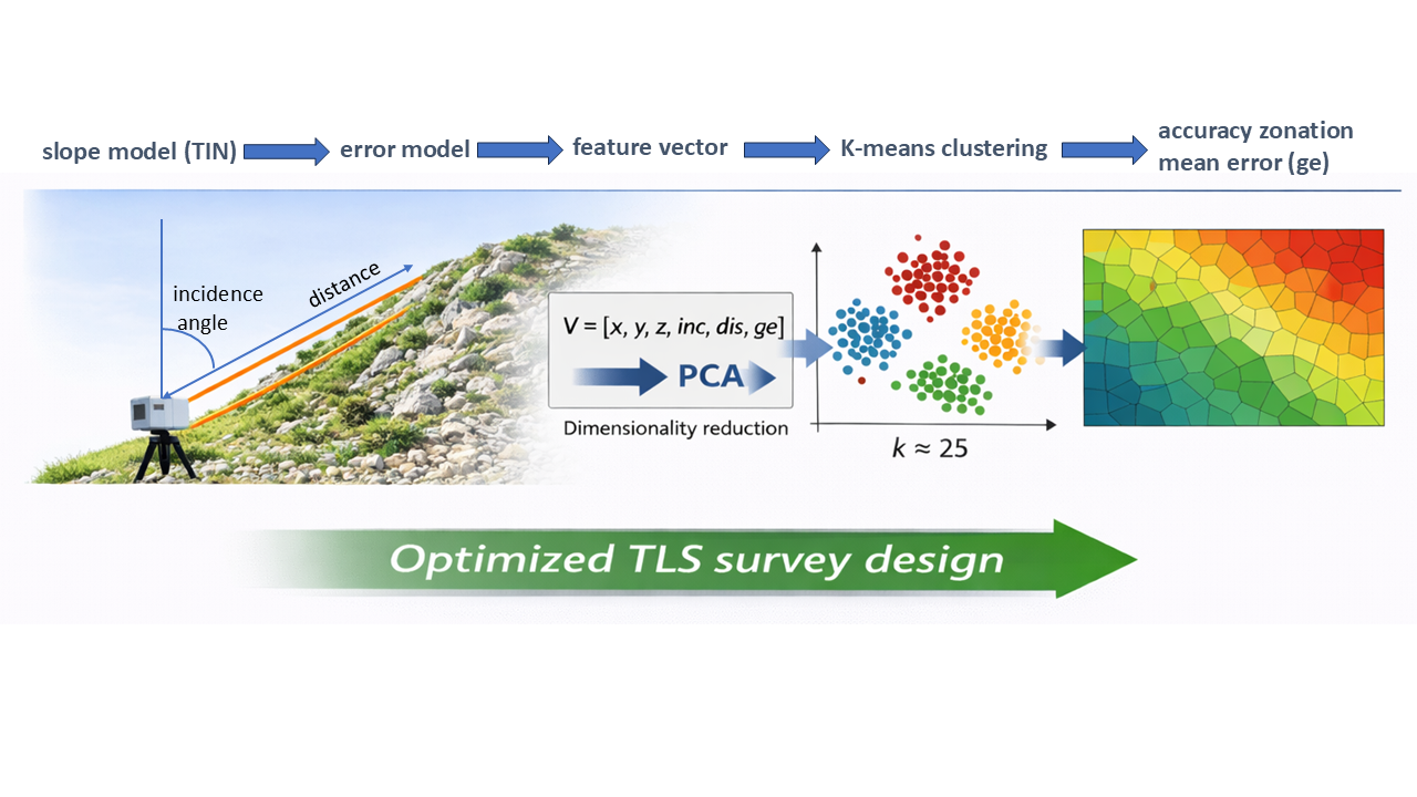
To overcome this limitation, the present work introduces a workflow that groups surface points into spatially coherent regions characterized by similar expected precision.

Given an approximate digital representation of the terrain, a Triangulated Irregular Network (TIN) is generated and candidate TLS station positions are defined. For each facet centroid, a positional error is simulated through an error model that incorporates instrument specifications and the geometric effects of beam divergence on inclined surfaces.

To analyse the spatial structure of these simulated errors, a multivariate variable is constructed that combines point position, error magnitude and the main geometric drivers of the error. Dimensionality reduction is performed using Principal Component Analysis (PCA), followed by clustering through the K-means algorithm to delineate zones expected to exhibit comparable measurement accuracy. This workflow constitutes a compact and fully unsupervised analytical pipeline, used here not to perform machine learning per se, but as a practical data-driven tool supporting TLS survey design.

Each cluster is then assigned to an error class, and the resulting spatial patterns can be compared across multiple candidate station positions. This allows identification of areas that can be surveyed within a desired accuracy threshold from a single station, as well as areas that require additional scans from alternative viewpoints.

The proposed workflow is structured as follows:

• Simulation of TLS measurements for both surface geometry and achievable precision, using an analytical error model;
• Association of each point with a multidimensional variable including spatial position, predicted error, and influencing parameters;
• Dimensionality reduction and clustering with a sufficiently large number of clusters to describe the spatial variability of the expected error;
• Re-aggregation of clusters into error classes to map areas characterized by distinct precision thresholds;
• Iterative simulation for different TLS stations to identify areas requiring multiple scans in order to achieve the desired accuracy.

This approach provides a systematic framework for the quantitative planning of TLS surveys in complex geomorphological environments.

2. Methods

To evaluate how the position of the TLS affects visibility and accuracy, the dataset that the instrument would acquire from a given station on the slope or landslide is first simulated.

2.1. Dataset Simulation

The general morphology of the surface is represented using a TIN (Triangulated Irregular Network) model, obtained through Delaunay triangulation.

Each triangle, defined by vertices $a_i,b_i,c_i$, represents a facet of the model; its centroid X_i is considered the point impacted by the laser beam.

Given the instrument position X_s, the vector from the instrument to the facet is $d{X}_i=X_i-X_s$.

For each point X_i, simulated pseudo-measurements can be calculated: azimuth angle θ, zenith angle ζ and distance ρ:

$$\theta =\arctan \left({\displaystyle \frac{dx}{dy}}\right); \rho =\sqrt{d{x}^2+d{y}^2+d{z}^2}; \zeta =\arccos \left({\displaystyle \frac{dz}{\rho }}\right)$$

(1)

The incidence angle between the facet normal ν_i and the direction of the beam vector $\delta ={\displaystyle \frac{d{X}_i}{\mid d{X}_i\mid }}$, is:

$$\mathrm{inc}=\arccos \left(\mathrm{\delta }·{\mathrm{\nu }}_{\mathrm{i}}\right); {\mathrm{\nu }}_{\mathrm{i}}={\displaystyle \frac{\left({\mathrm{a}}_{\mathrm{i}}-{\mathrm{b}}_{\mathrm{i}}\right)\times \left({\mathrm{c}}_{\mathrm{i}}-{\mathrm{b}}_{\mathrm{i}}\right)}{\mid \left({\mathrm{a}}_{\mathrm{i}}-{\mathrm{b}}_{\mathrm{i}}\right)\times \left({\mathrm{c}}_{\mathrm{i}}-{\mathrm{b}}_{\mathrm{i}}\right)\mid }}$$

(2)

Pseudo-measurements are computed to associate each point with an error consistent with the specifications of the assumed TLS instrument, including standard deviations ${\sigma }_{\theta },{\sigma }_{\zeta },{\sigma }_{\rho }$ and beam divergence γ.

Since instrument datasheets do not provide information on correlations between observations, these are assumed to be zero in the simulation. The variance matrix of the observations is:

$$\mathrm{diag}\left({\mathrm{\sigma }}_{\mathrm{\theta }}^2,{\mathrm{\sigma }}_{\mathrm{\zeta }}^2,{\mathrm{\sigma }}_{\mathrm{\rho }}^2\right)$$

(3)

The point variance is obtained using the law of error propagation [9], considering the Jacobian of the transformation from polar to Cartesian coordinates J_μX:

$${\Sigma }_{{\mathrm{X}}_{\mathrm{i}}}={\mathrm{J}}_{\mathrm{\mu }\mathrm{X}}\hspace{1em}{\Sigma }_{\mathrm{\mu }}\hspace{1em}{\mathrm{J}}_{\mathrm{\mu }\mathrm{X}}^{\mathrm{T}}$$

(4)

In addition to instrumental precision, beam divergence γ introduces an additional stochastic component, whose effect increases especially with the inclination of the facet.

The divergence parameter γ (full angle at the 1/e² intensity level) is modeled assuming a Gaussian radial energy distribution. The transverse standard deviation of the laser footprint at range $\mathrm{\rho }$ is:

$${\sigma }_{\rho }={\displaystyle \frac{\rho \gamma }{4}}$$

(5)

Following geometric models proposed in the literature, e.g., [8,10,11], beam divergence induces an intrinsic angular dispersion

$$\Delta {\sigma }_{\vartheta }=\Delta \sigma \varsigma ={\displaystyle \frac{\gamma }{4}}$$

(6)

and an additional range dispersion for a planar facet with incidence angle inc,

$$\Delta {\sigma }_{\rho }=\rho \tan \left(inc\right) \gamma /4$$

(7)

The augmented standard deviations are therefore modelled as

$${\sigma }_{\vartheta }^{\prime }=\sqrt{{\sigma }_{\vartheta }^2+{(\gamma /4)}^2};\hspace{1em}{\sigma }_{\varsigma }^{\prime }=\sqrt{{\sigma }_{\varsigma }^2+{(\gamma /4)}^2};\hspace{1em}{\sigma }_{\rho }^{\prime }=\sqrt{{\sigma }_{\rho }^2+{\displaystyle \frac{\rho tan\left(inc\right)\gamma }{4^2}}}$$

(8)

The updated covariance matrix is then propagated to Cartesian space as described above and the updated point variance becomes:

$${\Sigma }_{Xi}^{\prime }=J_{\mu X}\hspace{1em}diag\left({{\sigma }_{\vartheta }^{\prime }}^2,{{\sigma }_{\varsigma }^{\prime }}^2,{{\sigma }_{\rho }^{\prime }}^2\right)\hspace{1em}{J}_{\mu X}^T$$

(9)

A recent formulation [5] directly derives the point variance ${\Sigma }_{Xi}$ from the error ellipse defined by the laser footprint on the inclined facet.

The effect of beam divergence is modeled as a spatial uncertainty of the true scattering location over the laser footprint. On a planar facet inclined at angle inc, the footprint is approximated as an ellipse with semi-major axis a and semi-minor axis b.

Assuming a Gaussian intensity distribution, the footprint ellipse is defined at the 2σ level (≈95% confidence), so that $a=2{\sigma }_a$ and $b=2{\sigma }_b$. The corresponding standard deviations are therefore ${\sigma }_a={\displaystyle \frac{a}{2}}$ and ${\sigma }_b={\displaystyle \frac{b}{2}}$. This representation treats the beam divergence as a spatial uncertainty kernel distributed over the footprint, providing a physically consistent basis for propagating the measurement variance to the global reference frame.

In a local orthonormal reference frame aligned with the facet (axes along the semi-major, semi-minor directions, and the facet normal), the covariance matrix of the point location is: ${\Sigma }_{loc}^{\prime }=diag\left({\sigma }_a^2,{\sigma }_b^2,0\right)$

The local covariance is then rotated into the TLS reference frame:

$${\Sigma }_{TLS}=R{\Sigma }_{fac}{R}^T$$

(10)

where R is the rotation matrix from the facet frame to the TLS system. This formulation captures the anisotropic, orientation-dependent uncertainty due to beam divergence, e.g., [8,11].

To visualize the spatial variation of precision, we introduced a single scalar parameter expressed as a length. To retain the three-dimensional nature of the uncertainty, this parameter is defined as the square root of the mean of the coordinate variances, or the mean of the eigenvalues of the covariance matrix of the point coordinates

$$ge=\sqrt{{\displaystyle \frac{{\sigma }_x^2+{\sigma }_y^2+{\sigma }_z^2}{3}}}=\sqrt{{\displaystyle \frac{{\lambda }_1+{\lambda }_2+{\lambda }_3}{3}}}$$

(11)

This corresponds to the standard deviation of an equivalent isotropic uncertainty having the same total variance as the original 3D error distribution.

This approach enables mapping the spatial distribution of expected precision, identifying homogeneous accuracy zones through direct filtering or clustering (e.g., K-means).

Similarly, planimetric error $ep=\sqrt{{\displaystyle \frac{{\sigma }_x^2+{\sigma }_y^2}{2}}}$ and vertical error $e_h={\sigma }_z$.

The method provides the predicted spatial distribution of measurement uncertainty across the modeled surface.

The goal is to identify zones with homogeneous error characteristics rather than isolated anomalies.

Two complementary aggregation strategies have been implemented:

• A data-driven clustering approach (e.g., K-means) applied to the multidimensional variable V = [x, y, z, ge, inc, dis].
• A direct filtering and visualization approach using standard GIS tools.

2.2. Clustering with K-Means

To identify well-defined portions of the object where the simulated error parameter is spatially homogeneous, a clustering analysis is performed using the K-means algorithm.

2.2.1. Aggregated Variable and Preprocessing

The variable used for clustering accounts for both the three-dimensional position of each point and the positional error, along with the parameters that most influence it—namely, the distance and the angle of incidence on the reflective surface. The variable is defined as: V = [x, y, z, ge, inc, dis].

This multidimensional variable includes three components related to spatial position and three related to error. Not all components have the same impact on the clustering process due to existing correlations among variables and differing value ranges (hundreds of meters for spatial coordinates, decimeters for error, and tens of degrees for the angle of incidence).

To mitigate these effects, standardization and/or weighting of the individual components of V can be applied prior to dimensionality reduction, using techniques such as PCA (Principal Component Analysis) or UMAP (Uniform Manifold Approximation and Projection).

Both algorithms are sensitive to variable scaling—PCA due to its dependence on variance, and UMAP due to distortion in the neighborhood graph constructed from distances.

A commonly recommended procedure [12,13] is to standardize the components of the variable, resulting in dimensionless values with zero mean and unit variance. However, since the value ranges remain different, it is advisable to introduce weights that account for these differences. This approach is referred to here as KMNorm.

Even though clustering with K-means is performed in a reduced-dimensional space, assigning greater weight to the spatial coordinates promotes the formation of more compact and geographically coherent clusters. It has been observed that without coordinate weighting, the resulting clusters exhibit significant spatial overlap.

The appropriate weight to apply to the coordinates can be derived from the ratio of their ranges relative to the other components. While standardization is considered a gold standard in the literature, it is also useful to test an alternative approach, referred to here as KMNoNorm, which involves assigning a weight to the ge component. This component has a much smaller range compared to the coordinates in typical applications, so the weighting in this case is applied to the error rather than the coordinates.

Specifically, the error parameter ge was multiplied by a factor of 100, in order to align the order of magnitude between the spatial coordinate range (hundreds of meters) and the error range (meters). This corresponds to expressing error values in centimeters rather than meters, thereby aligning the order of magnitude of spatial and error-related variables without altering their internal structure.

The goal remains to identify clearly distinguishable clusters in 3D space, within which the surveyor can make informed decisions.

2.2.2. Dimensionality Reduction and Correlation Attenuation

As the dimensionality of the feature space increases, distance metrics tend to lose their significance as measures of similarity, since the relative differences between distances progressively diminish. This phenomenon, commonly referred to in the literature as the curse of dimensionality [14,15], results in data points becoming nearly equidistant from one another, thereby reducing the ability of distance-based algorithms such as K-means to identify clear separations between clusters.

Although the number of variables considered in this study is relatively small (six), and thus does not constitute a high-dimensional space in the strict sense, their heterogeneity still leads to reduced discriminative power of K-means, making dimensionality reduction advisable.

To reduce the dimensionality of the problem, Principal Component Analysis (PCA) can be employed. PCA transforms the original set of variables into a new set of mutually uncorrelated components. Among these, only the few that retain the majority of the information—typically those explaining at least 95% of the variance—are considered. In most cases, 2–3 principal components are sufficient.

PCA also allows for the analysis of the correlation levels among the original variables and between these and the selected principal components, which are subsequently used for clustering, provided that the explained variance is sufficiently high. An effective graphical representation of this relationship can be obtained, for example, using the “biplot” function in MATLAB (R2025a, The MathWorks, Inc., Natick, MA, USA).

2.2.3. K-Means Clustering: Determining the Number of Clusters

Once the dimensionality of the problem has been reduced, clustering is performed using the K-means algorithm, which partitions the original dataset into k subgroups by minimizing the within-cluster sum of squares (WCSS) between individual points and the centroid of their respective cluster:

$$WCSS={\displaystyle {\sum }_j^k}{\displaystyle {\sum }_{i\in Cj}{\left|\right|x_i-{\mu }_j\left|\right|}^2}$$

(12)

where μ_j is the centroid of cluster C_j.

The algorithm is iterative, can use various distance metrics, but requires the number of clusters k to be defined a priori.

For the purposes of this study, a relatively large number of clusters—in the order of several tens—is chosen to identify areas with distinct precision characteristics.

Broadly speaking, the number of clusters corresponds to the “resolution” of the method: the larger the number, the more it allows for capturing variations in the analyzed variables. In other words, a greater number of clusters improves adaptation to the slope’s morphology.

To assist in selecting the optimal k, several well-established indices from the literature are used [16,17], which evaluate cluster compactness and separation. In summary:

-

Silhouette Index (SI)

Measures how similar each point is to its own cluster compared to others.

$$S{I}_i=\left(b_i-a_i\right)/\mathit{max}\left(b_i-a_i\right)$$

(13)

where a_i is the average intra-cluster distance and b_i is the lowest average inter-cluster distance.

The mean Silhouette value ranges from −1 (poor clustering) to 1 (excellent clustering).

-

Davies–Bouldin Index (DBI):

Measures the average similarity between clusters.

$$DBI={\displaystyle \frac{1}{k}}{\displaystyle \sum }_{i=1}^k\underset{j\ne i}{max}\left({\displaystyle \frac{{\sigma }_i+{\sigma }_j}{d_{ij}}}\right)$$

(14)

where σ_i is the average intra-cluster distance and d_ij is the distance between centroids.

Lower values indicate better clustering.

-

Calinski–Harabasz Index (CHI):

Expresses the ratio between inter-cluster and intra-cluster variance:

$$CHI={\displaystyle \frac{tr\left(B_k\right)/\left(k-1\right)}{tr\left(w_k\right)/\left(n-k\right)}}$$

(15)

where B_k and W_k are the between- and within-cluster dispersion matrices.

Higher values correspond to more distinct and compact clusters.

-

Dunn Index (DI).

Defined as the ratio between the minimum inter-cluster distance and the maximum intra-cluster diameter:

$$DI={\displaystyle \frac{\underset{\mathrm{i}\ne j}{min} d\left(C_i,C_j\right)}{\underset{k}{max} \delta \left(C_k\right)}}$$

(16)

where d(C_i,C_j) is the distance between clusters i and j, and δ(C_k) is the diameter of cluster k.

Higher Dunn values indicate better separation and compactness.

It is important to note that computing the Dunn index is computationally intensive for large datasets, so its use is recommended on smaller subsets.

These indices provide complementary perspectives: Silhouette and Dunn favor compact, well-separated clusters, while Calinski–Harabasz and Davies–Bouldin focus on overall variance structure.

It is recommended to compute all these indices across a range of k values. In the test case, the interval from 5 to 80 with a step of 5 was used.

The optimal k corresponds to a balance between internal cohesion and external separation—that is, the point where the quality indices stabilize or reach their extremal values.

Once the points are assigned to clusters, statistical measures of the global error ge are computed to associate a meaningful value with each cluster. For simplicity, the mean or median can be used.

It is important to note that in the considered application, due to the highly variable inclination of the facets, clusters may contain values significantly higher or lower than the average.

2.2.4. Value Ranges of the Central Parameter

Since it is generally of interest to determine whether the survey achieves a certain level of precision (e.g., “medium”) or at least to identify the portion of terrain where such precision can be reached, the method proceeds by identifying macro-areas corresponding to a mean error parameter falling within predefined thresholds.

A classification is introduced based on a set of intervals—not necessarily of equal width—of the mean error associated to each cluster. Adjacent polygons with different mean errors but belonging to the same class can then be spatially aggregated into a single macro-area.

This can be performed in a GIS environment using procedures such as the “polygon dissolve operation”.

In the following, this operation will be referred to simply as dissolve, in accordance with the terminology commonly adopted in GIS software such as ArcGIS and QGIS. More broadly, these operations conceptually fall within the framework of vector generalization and overlay processing in GIS [18,19].

It should be noted that the width of the intervals—and consequently the number of resulting classes—contributes to defining the resolution of the method and must therefore be evaluated on a case-by-case basis, considering the characteristics of the dataset under analysis.

2.3. Simulation Comparison

If a single TLS station allows the desired error threshold to be achieved, the simulation is considered complete.

Otherwise, by repeating the same procedure for additional station positions, it is possible to integrate the areas that meet the threshold and verify whether the selected stations collectively achieve the required (average) level of precision.

This procedure can be easily performed within a GIS environment using the following sequence of operations:

-

The polygons corresponding to the macro-areas obtained from the various simulations are combined using the Merge tool—a commonly used term for combining multiple layers into a single dataset.

-

Those clusters with an error class below the predefined threshold are selected and subsequently subjected to further spatial aggregation through the Dissolve tool.

It should be noted that in this case, the dissolve operation serves not only to ensure spatial continuity among polygons belonging to the same class, but also to resolve overlaps resulting from the combination of multiple simulations.

2.4. Clustering with an Ad Hoc GIS Approach (AHG)

When it is not possible to process the data using the previously described K-means approach, a simplified procedure can be adopted within a GIS environment to obtain a rapid coarse aggregation of the simulated error (hereafter referred to as the ad hoc GIS approach, AHG).

This approach is inspired by [20], but has been substantially revised and extended for the present study. It is implemented here using ESRI ArcGIS Pro (version 3.5, Esri, Redlands, CA, USA, tool names refer specifically to this software), although it can also be carried out in other GIS platforms and potentially automated in Python. The working environment consisted of a PostgreSQL database with the PostGIS spatial extension.

The procedure involves discretizing the error by defining a vector grid superimposed on the TIN facets. For each grid cell, the mean error value of the intersecting facets is calculated, weighted by the area proportion of each triangle portion contained within the cell. The cells are then classified according to their mean error and dissolved by class. The number of classes corresponds to the number of groups intended to be obtained. The output consists of polygons associated with the same mean error value.

The grid spacing acts as a step filter: as the cell size increases, the smoothing effect on the errors associated with the points contained within the cell also increases, and consequently the variance of their distribution.

The main steps of the procedure are summarized as follows:

• Determination of the envelope of the facets, defined as the smallest axis-aligned rectangle (bounding box) that fully contains them.
• Generation of a vector grid matching the extent of the envelope, composed of square cells with a side length of 10 m.
• Spatial overlay (Identity operation) between the facets and the grid, resulting in the subdivision of each grid cell into one or more portions corresponding to the intersecting facets.
• Import of the resulting identity table into a relational database with spatial extension, such as PostgreSQL or Oracle. A group by query on the identifier of each grid cell allows computation of the average error of the facet portions falling within it, weighted by their area. A subsequent query performs classification into 10 classes ranging from 0 to 0.5 m, with 5 cm intervals, plus a residual class for all errors greater than 0.5 m.
• The classified table is then joined back to the original grid and dissolved by class to obtain contiguous areas of similar accuracy.
• Defining a certain error threshold allows the merging and dissolving all classes below it, thereby delineating homogeneous areas with acceptable precision.
• Optionally, a final fill gaps step may be performed to simplify the extraction of cluster polygon boundaries.

In the case of multiple simulations corresponding to different TLS stations, the procedure can be repeated for each of them. The classified grids can then be merged into a single dataset. Conceptually, this operation corresponds to point cloud coregistration.

A SQL query manages overlapping cells by retaining those with the lower classification value. Finally, a dissolve operation aggregates the output cells belonging to the same class, thereby defining the cluster polygons. As with the K-means approach, it is possible to set an error threshold and identify the cluster polygons below it, eventually dissolving them into a single output polygon.

3. Test Case

The study area considered is a portion of a landslide-affected slope, located at elevations ranging from 80 to 330 m above sea level, and has already been the subject of previous studies [21,22]. Specifically, the terrain considered in the simulation corresponds to the western slope of Monte Castello, located in the municipality of Castel San Giorgio (Italy), as shown in Figure 1.

Large portions of the area are almost entirely devoid of vegetation (Figure 2a), while the upper section features a rocky escarpment affected by both tectonic discontinuities (joints and faults) and sedimentary structures (bedding planes), which influence its mechanical properties and stability (Figure 2b).

In addition to multi-scale cartographic datasets, the area is covered by an Aerial Laser Scanner (ALS) survey conducted by the Italian Ministry of the Environment and Energy Security [26].

The slope’s elevation data are derived from the ALS surface point cloud (average density: 1.5 points/m²; declared vertical accuracy: 15 cm), georeferenced in the National Geodetic System.

This point cloud provides a top-down representation of the area, unaffected by ground-level perspective.

Based on the cartographic representation of the study area, candidate TLS stations positions are selected. Once the coordinates are extracted from the map, their corresponding positions on the terrain can be determined using NRTK surveys referenced to the national network of permanent GNSS stations.

This means that the points selected for simulation can be physically located on-site to perform the actual scan corresponding to the simulation.

From each hypothetical station, a corresponding field of view is identified. Figure 3 shows the areas analyzed from three different stations. The northern boundary is defined by the summit of the slope.

4. Processing and Results

4.1. Simulation of Test Case Data Sets and Filtering

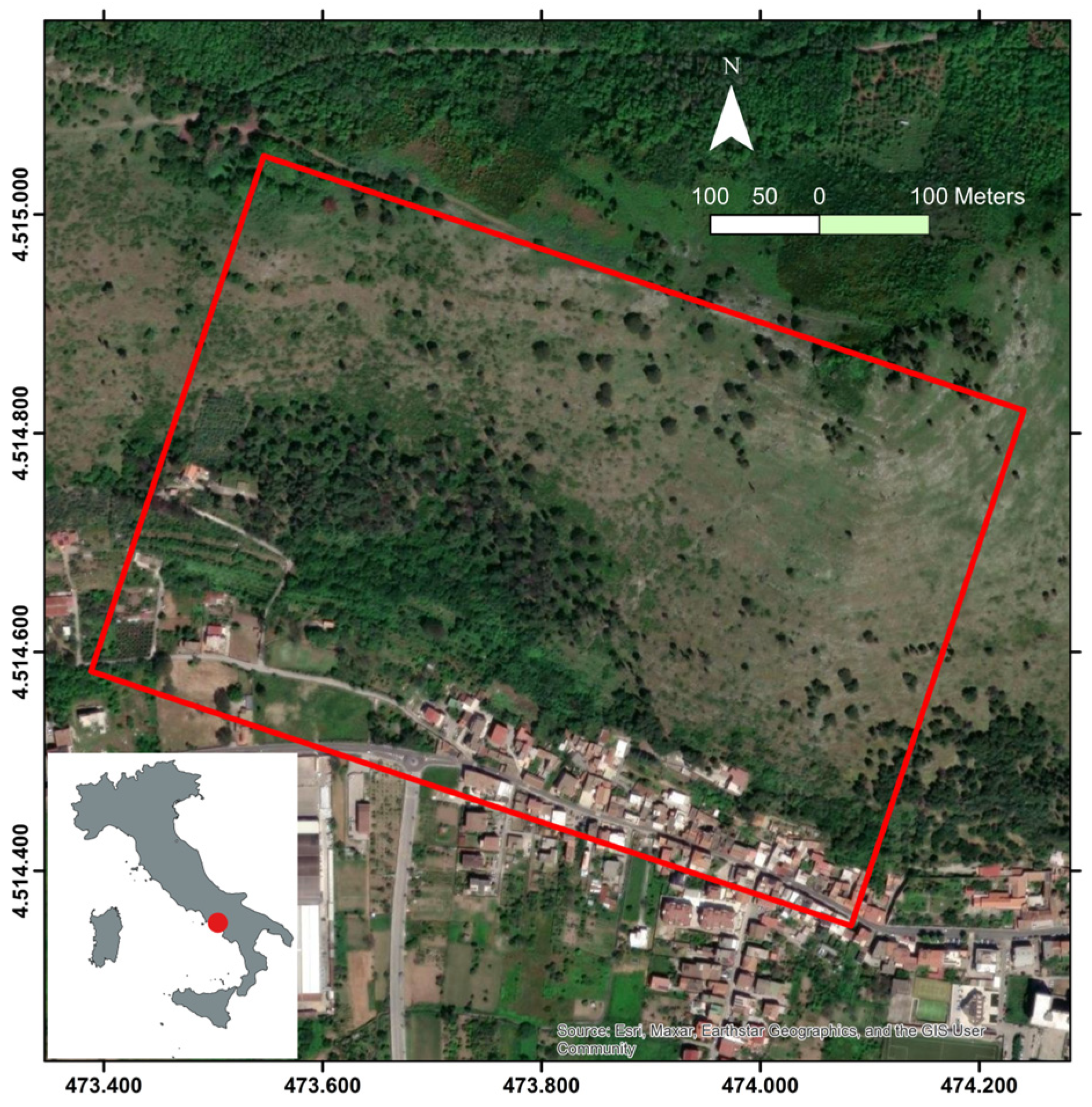
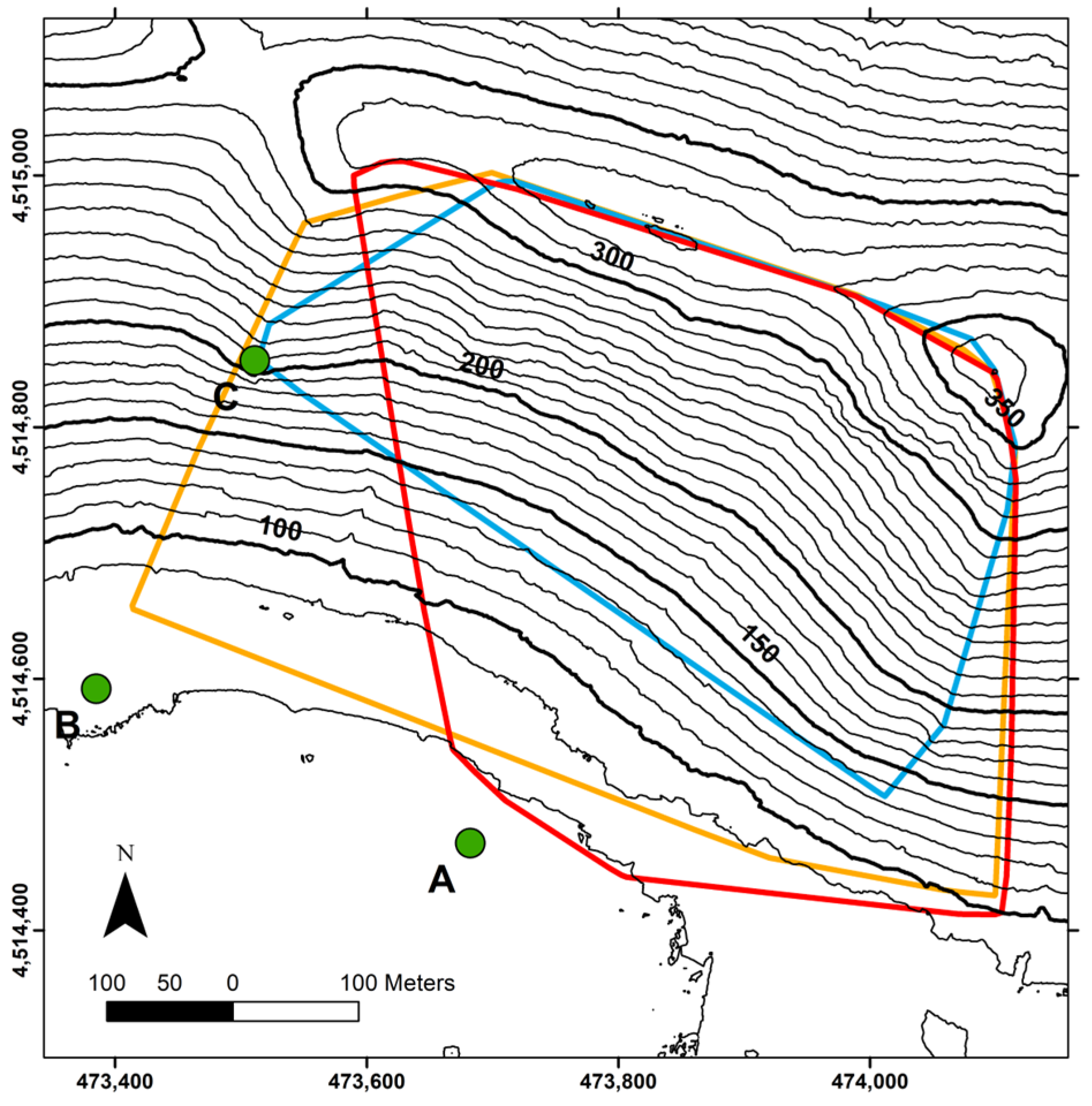
In the test case, the ALS point cloud was used to generate the TIN under three different TLS positioning hypotheses. Each TIN consists of approximately 200,000 facets, whose centroids are considered as simulated points. From the TIN, both the inclination angle (inc) of each facet and the centroid–instrument distance (dis) are derived.

The selected error model allows the assignment of a global error (ge) to each point, thus defining the variable V = [x, y, z, ge, inc, dis] for all facets visible from the station.

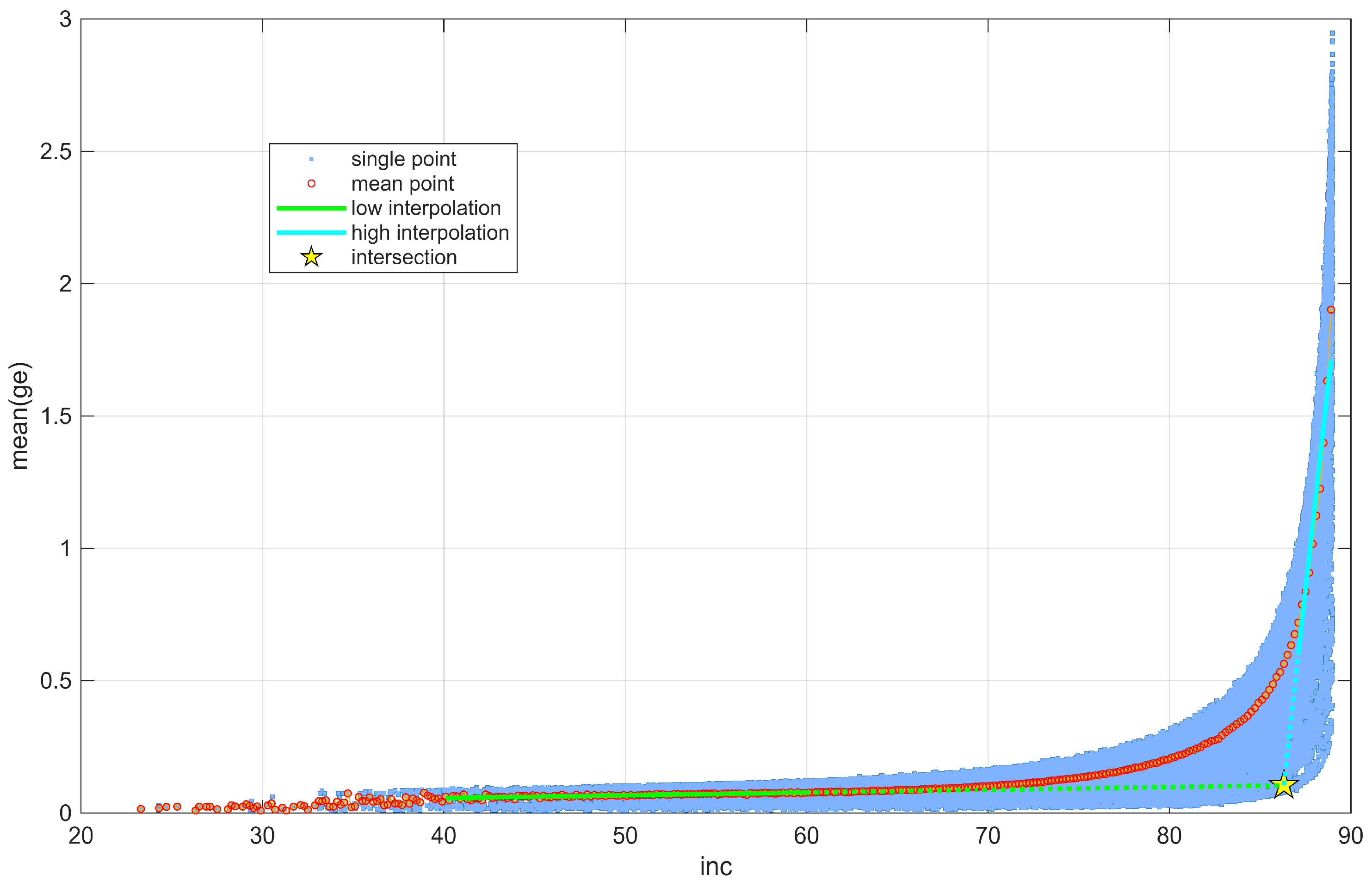
The value of ge shows a strong dependence on the incidence angle inc as illustrated in Figure 4 for all simulated points (grey dots). To highlight the underlying trend, the mean ge was computed within angular bins of width Δinc = 0.2°, these averaged values are shown in red. After an initial weakly increasing linear behaviour, the curve exhibits a marked steepening.

To determine a reference value of inc corresponding to this transition (“elbow”), two angular ranges where the relationship appears approximately linear were selected:

a slow-growth segment (inc = 40°–60°) and a terminal steep segment (inc > 87°).

Straight lines fitted to these two ranges intersect at a point (yellow star in Figure 4), whose abscissa is taken as the threshold angle inc* i.e., the point at which the trend changes.

For the three simulated datasets, nearly identical values were obtained:

inc* = 86.30°, 86.28°, 86.36°.

The uncertainty of the estimated intersection coordinate inc* = was evaluated using a non-parametric bootstrap approach. For each branch, bootstrap samples were generated by resampling the original data (inc, mean_ge) pairs with replacement while preserving the sample size. Linear regressions were recomputed for each replicate, and the corresponding intersection point was calculated.

Repeating this procedure 10,000 times produced an empirical distribution of inc* and its standard deviation was adopted as the standard uncertainty of the estimated threshold angle.

The resulting uncertainties for datasets A, B, and C were very similar: 0.1°, 0.2°, 0.2° respectively.

Based on these considerations, a data filter was applied at inc = 86°, which reduces the sample by approximately 2% and results in sub-metric values of ge.

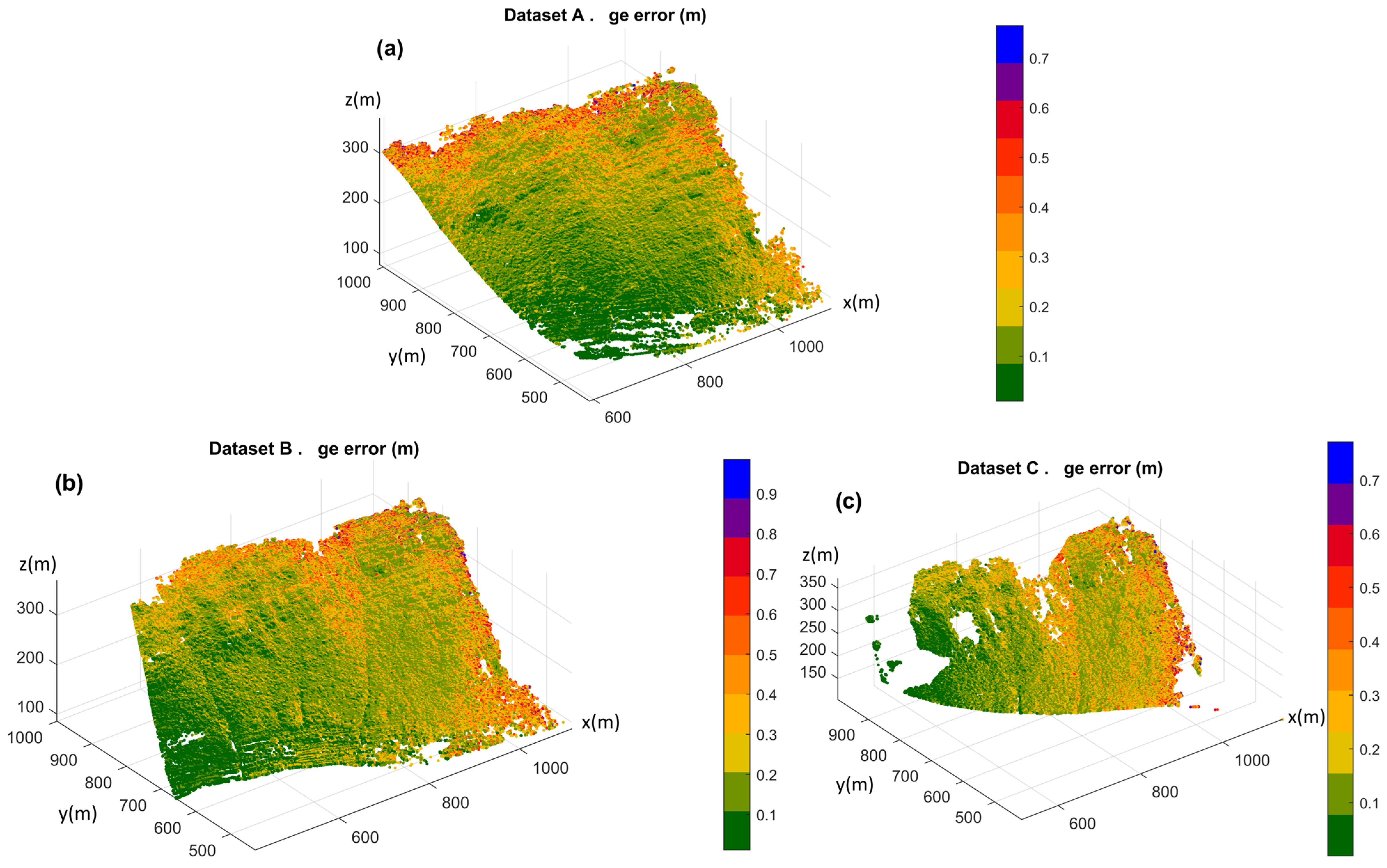
The 3D representation of individual error values, thematically colored, Figure 5, does not allow the identification of an area where a specific value is predominantly present.

4.2. Variable Treatment for Dimensionality Reduction

To delineate areas characterized by a specific error level, clustering was performed on the variable V = [x, y, z, ge, inc, dis].

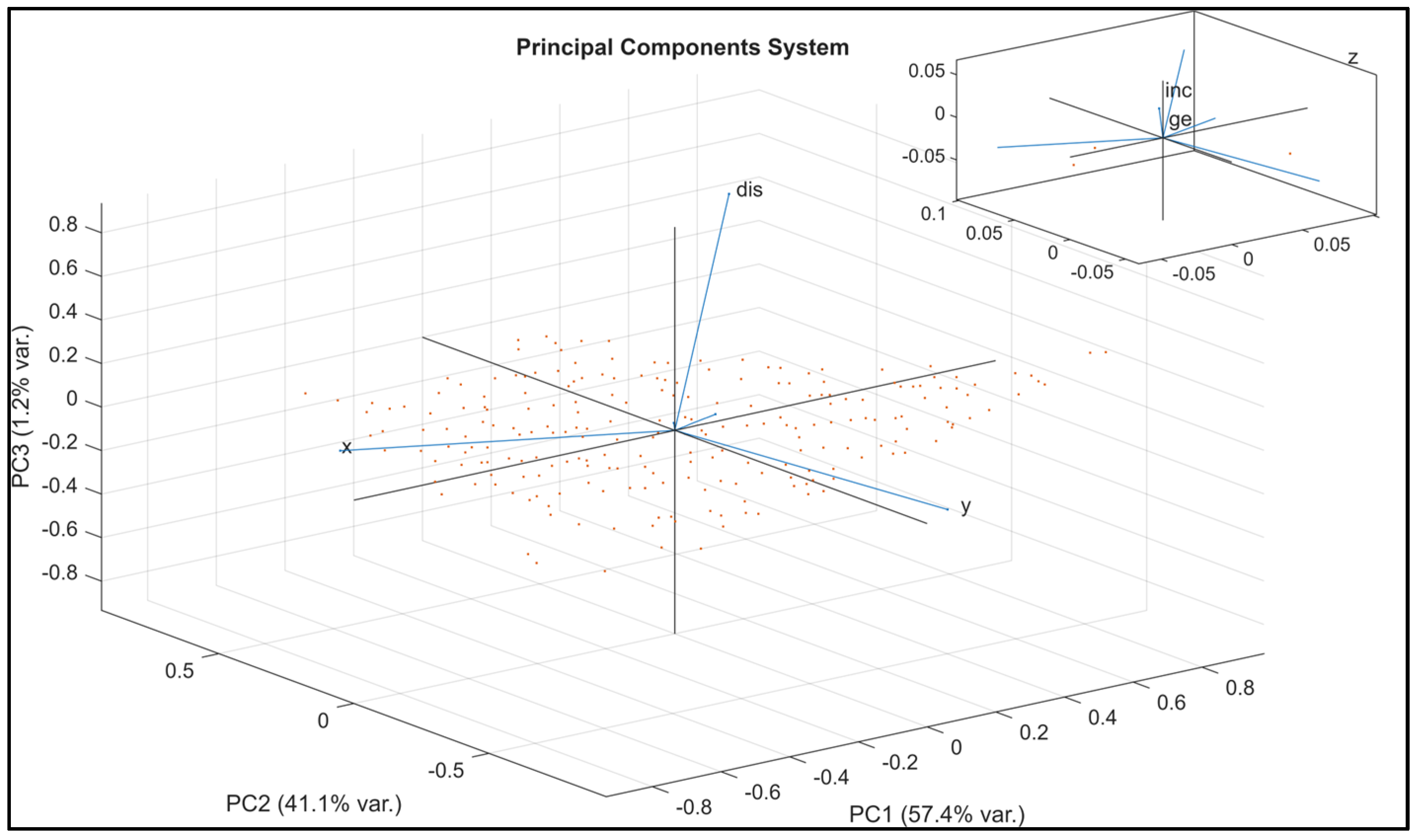
Since the six components of the variable are partially correlated, dimensionality reduction was applied prior to clustering, using Principal Component Analysis (PCA). For dataset A, the first three Principal Components (PCs) obtained through PCA account for more than 99% of the cumulative explained variance, and therefore the analysis was conducted on these three eigenvectors.

A representation of the six original variables in the space of the three PCs, known as a biplot, is shown in Figure 6. The points displayed correspond to a sub-sample of dataset A reduced by a factor of 1000 to improve readability.

The length of the vectors representing the variables indicates the degree of correlation with the principal components, while the angle between each vector and a PC axis shows the correlation of the variable with that component—zero if orthogonal. The angle between two vectors, instead, indicates the correlation between the original variables.

It should be noted that PCA favors components with larger ranges, which in this case differ considerably. Moreover, clustering must preserve both the spatial location of the identified clusters and their separability; for this purpose, weights can be assigned.

An initial approach consisted of applying the commonly suggested procedure of variable standardization (mean = 0, standard deviation = 1). However, the range of standardized values remains different: the range of ge is nearly twice that of the coordinate variables, as shown in

Table 1. Range of the standardized components of the analyzed variable.

Standardized	x	y	z	ge	inc	dis
A	4.0	4.2	4.4	7.2	8.8	5.4
B	4.3	4.9	4.0	11.7	7.8	5.1
C	4.9	5.9	4.4	11.8	8.8	5.8

.

As a “rule of thumb,” in this approach a double weight was assigned to the coordinate variables compared to the other components, in order to better identify the spatial location of the resulting clusters.

A second approach directly uses the dimensioned variables, whose ranges are reported in

Table 2. Range of the components of the analyzed variable (m, deg).

Original t	X (m)	Y (m)	Z (m)	ge (m)	inc (deg)	dis (m)
A	525.3	595.5	291.5	2.9	70.6	582.7
B	1190.7	1085.0	283.7	3.9	64.2	734.4
C	632.6	581.0	267.5	3.0	69.0	776.0

.

Since the ranges are much larger for the coordinates, to balance the weight of the components the error parameter ge was multiplied by a factor of 100, effectively expressing it in centimeters—again following a “rule of thumb.”

4.3. Choice of the Number of Clusters

The use of the K-means algorithm requires the number of clusters k to be selected a priori. In this application, the number of clusters cannot be reduced to just a few units, as sufficient spatial “resolution” must be preserved: the larger the number of groups, the better the adaptation to slope morphology.

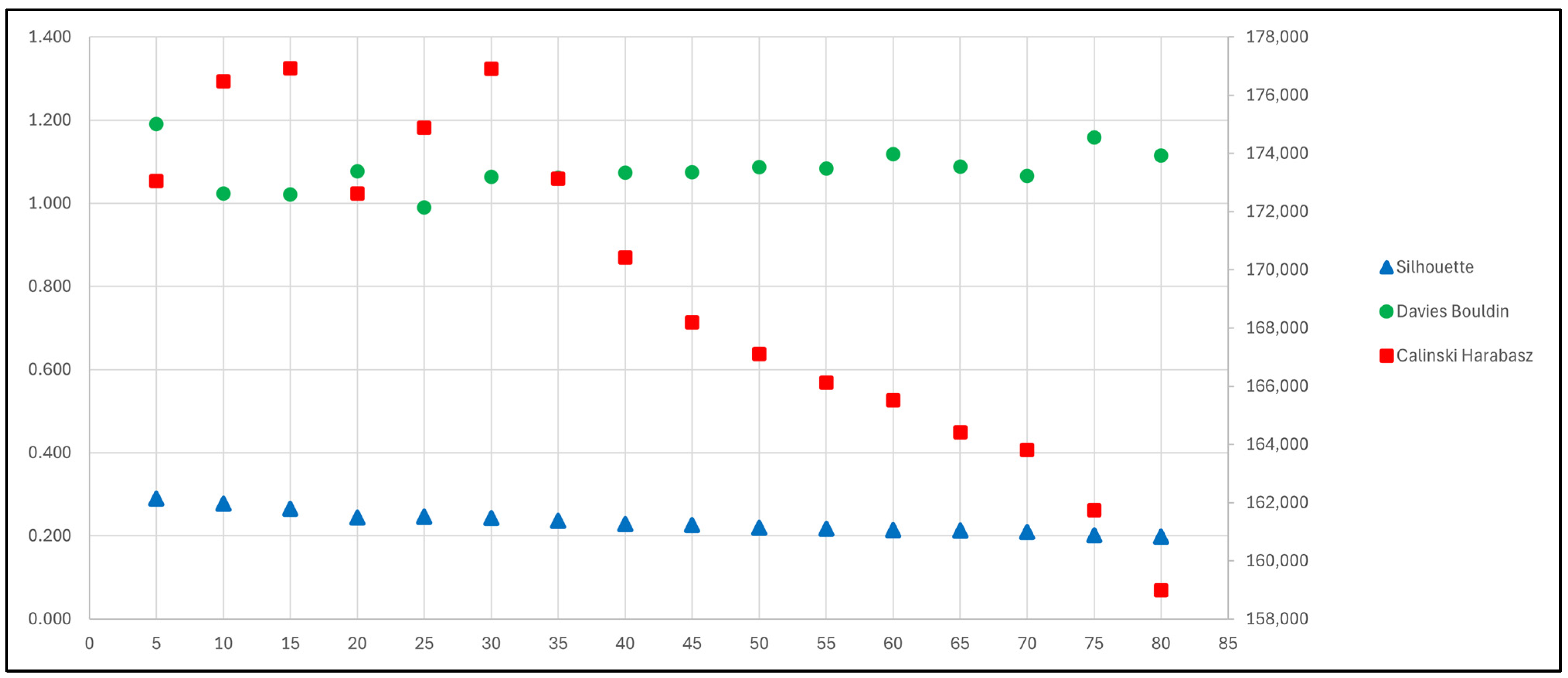
To identify a value of k that produces clusters that are both internally compact and externally well separated, the Silhouette, Davies–Bouldin, and Calinski–Harabasz indices were computed in the terrain-coordinate space for a variable number of clusters ranging from 5 to 80, with a step of 5. The resulting values for the entire dataset A are shown in Figure 7.

From the comparison of the indices, k = 25 was selected as a suitable number of groups. Since no single index provides a universally optimal value of k, the final choice was based on the combined interpretation of the three metrics. This value represents a compromise where the indices jointly indicate a satisfactory balance between cluster compactness and separation, avoiding both the excessive generalization associated with too few clusters and the artificial fragmentation that may arise when the number of partitions becomes too large. In particular:

-

Silhouette (the higher, the more compact and well-separated the groups): the index shows a gradual decrease as k increases, which is a typical behavior when the number of clusters grows. Around k = 25, the value remains relatively high while still preserving meaningful cluster compactness.

-

Calinski–Harabasz (the higher, the more separated and compact the clusters): the index reaches high values in the range between approximately k = 10 and k = 30, indicating good separation among clusters. Beyond this interval, the index shows a marked decrease, suggesting that further increasing the number of clusters does not improve the partition quality. Selecting k = 25 therefore falls within this favorable interval while avoiding an excessive increase in model complexity.

-

Davies–Bouldin (the lower, the more dissimilar the clusters): the index shows a local minimum around k = 25, after which it increases again, indicating a progressive rise in the average similarity between clusters and therefore a reduction in cluster separation.

4.4. Spatial Distribution of Clusters

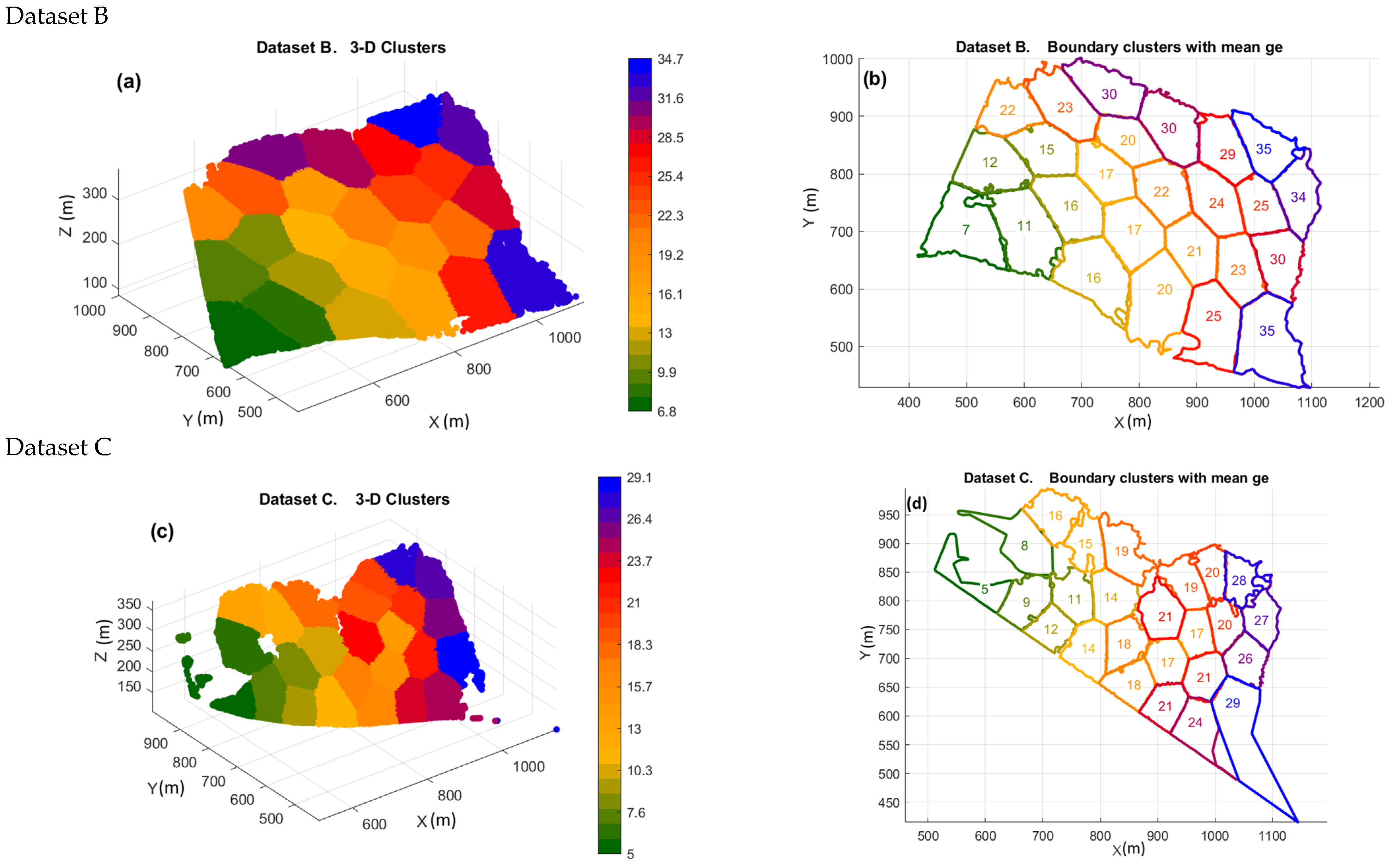
The K-means algorithm assigns each data point uniquely to one of k clusters. Each cluster is then associated with a parameter representing the prevailing error level of the points belonging to that cluster. The mean value of ge was selected as the representative parameter. The use of a more robust centrality estimator, such as the median, does not lead to significant differences and does not simplify interpretation. The clusters are then numbered according to the increasing value of the associated parameter.

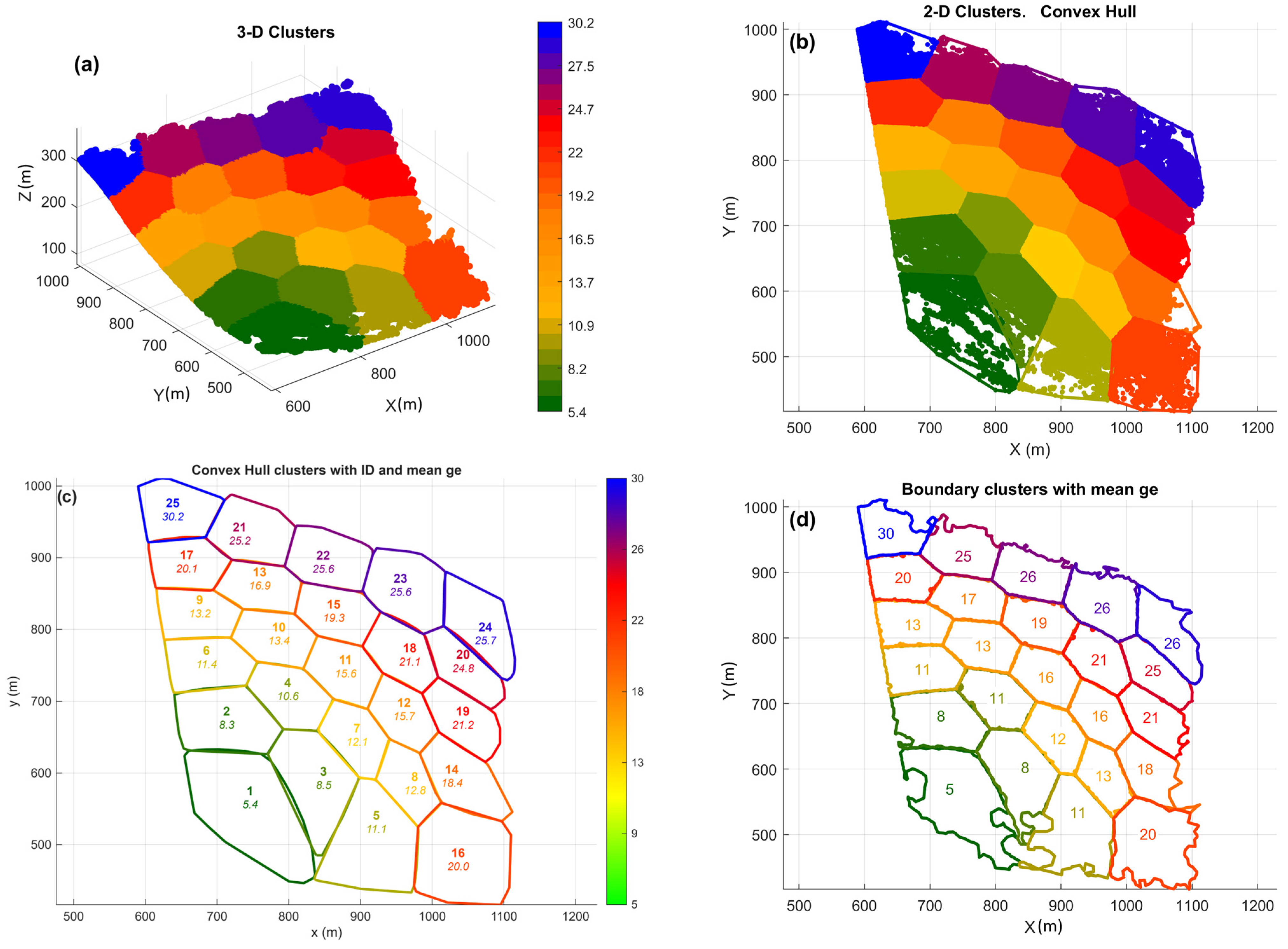
For dataset A, the spatial distribution of clustered points is shown in Figure 8. Specifically, panels (a) and (b) display the 3D and 2D spatial distributions with a color scale representing the parameter associated with each cluster. Panel (c) shows the 2D contour obtained using the Convex Hull algorithm [27], with the value of the central parameter (in cm) and the cluster order number indicated inside. Panel (d) presents the contour delineation obtained with a different algorithm (the MATLAB boundary function) [28,29], which defines the contour with a larger number of boundary points; the associated parameter value is reported within the polygon.

The color scale allows visualization of the indicative trend of the error associated with each cluster, bearing in mind that it refers to a mean value and that individual points within each cluster may exhibit different values of ge (Figure 9). These are mainly related to the configuration of individual facets that deviate from the trend of surrounding facets within the cluster.

Similar patterns are observed for datasets B and C, aggregated using the same number of clusters.

4.5. GIS Approach (AHG)

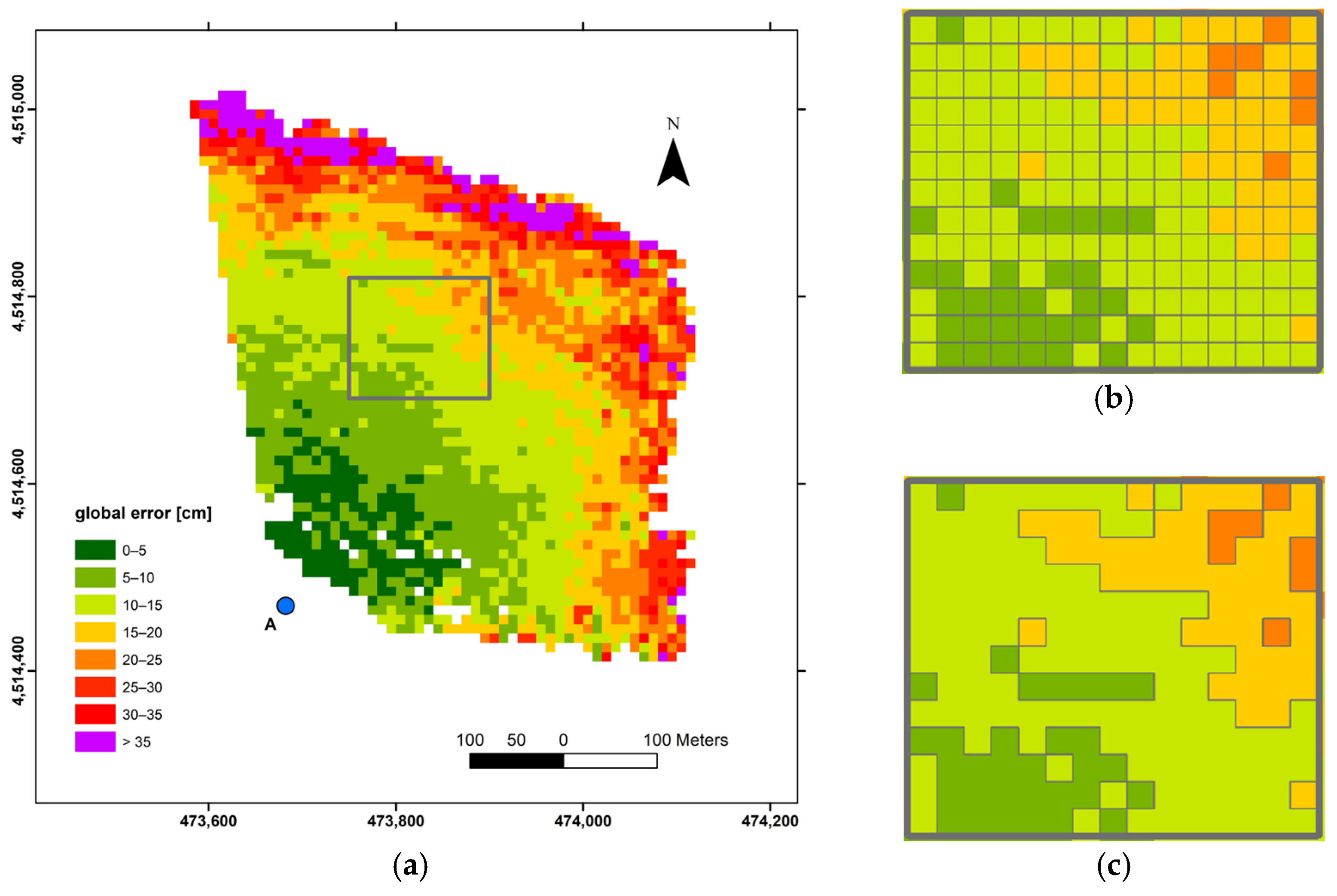
Even the discretization according to the AHG approach of the facets visible from station A, by itself, does not allow for the delimitation of homogeneous and spatially continuous areas characterized by a certain global error. For visualization purposes only, a classification of the error associated with the cells (Figure 10a) might be sufficient. However, to perform quantitative evaluations, a subsequent dissolve is required, based either on a field corresponding to the classification or on the position of the values relative to a given error threshold.

The dissolve operation allows the identification of macro-areas characterized by a given level of accuracy, conceptually equivalent to the groups obtained with the K-means approach. This procedure can be applied both to a single simulation and to the merging of the three simulations. In the latter case, the dissolve also makes it possible to avoid spatial overlaps between cells occurring in more than one simulation ().

4.6. Cluster Merging by Ranges of the Central Parameter

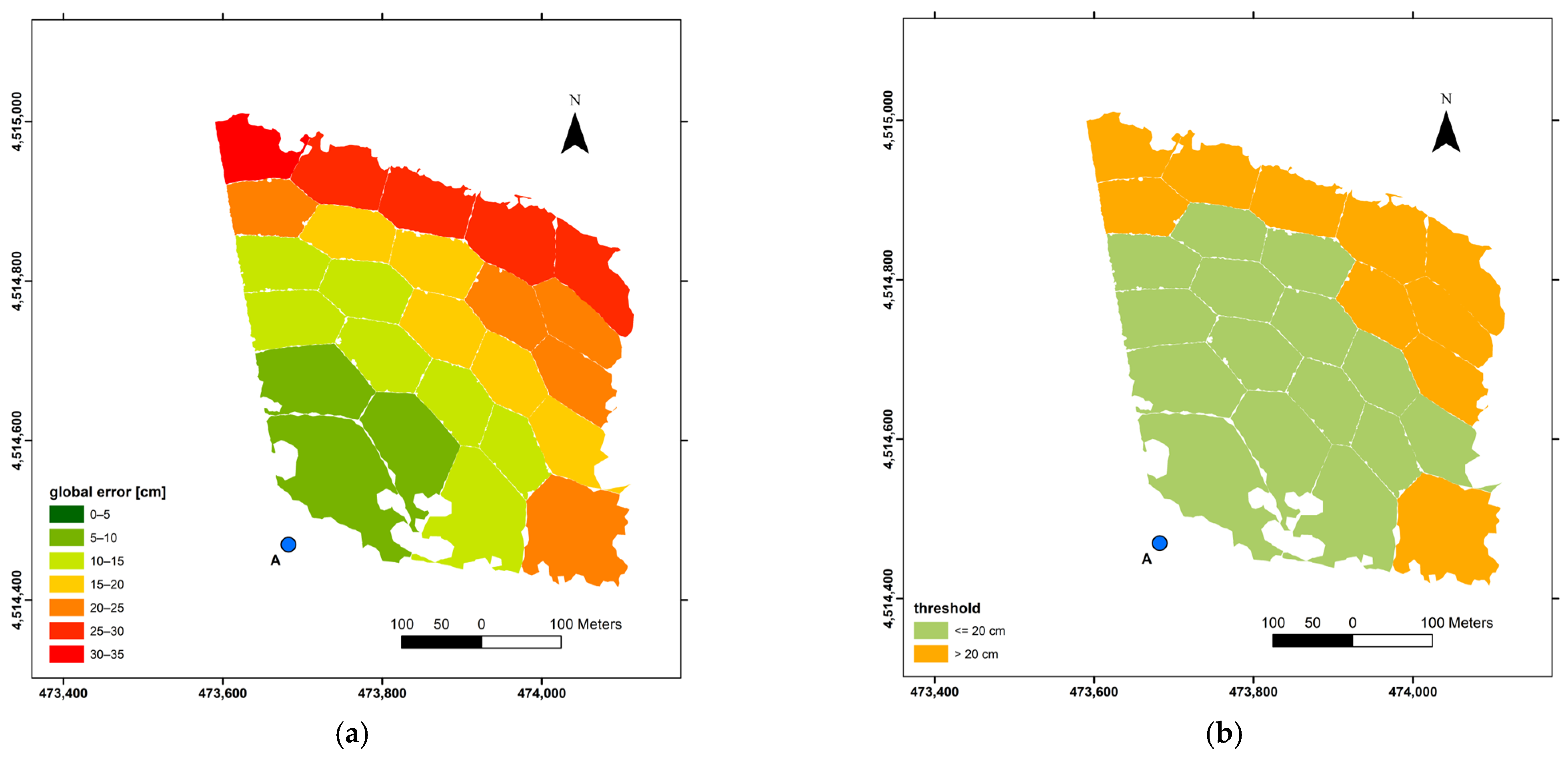
Once the K-means approach was identified as providing the best spatial aggregation, the clusters were classified into intervals of mean cluster error, similar to the GIS-based approach. These clusters were then further spatially aggregated within a GIS environment using the Dissolve tool.

This step allows the identification of macro-areas covered with a given level of precision (Figure 11).

Analogous results were obtained for datasets B and C.

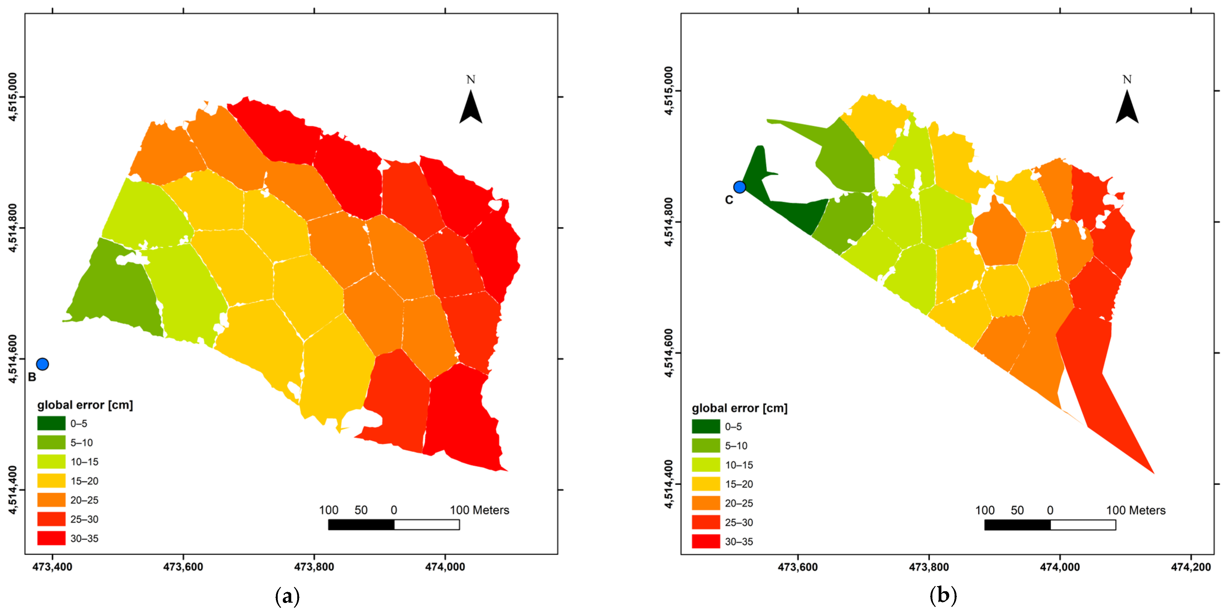
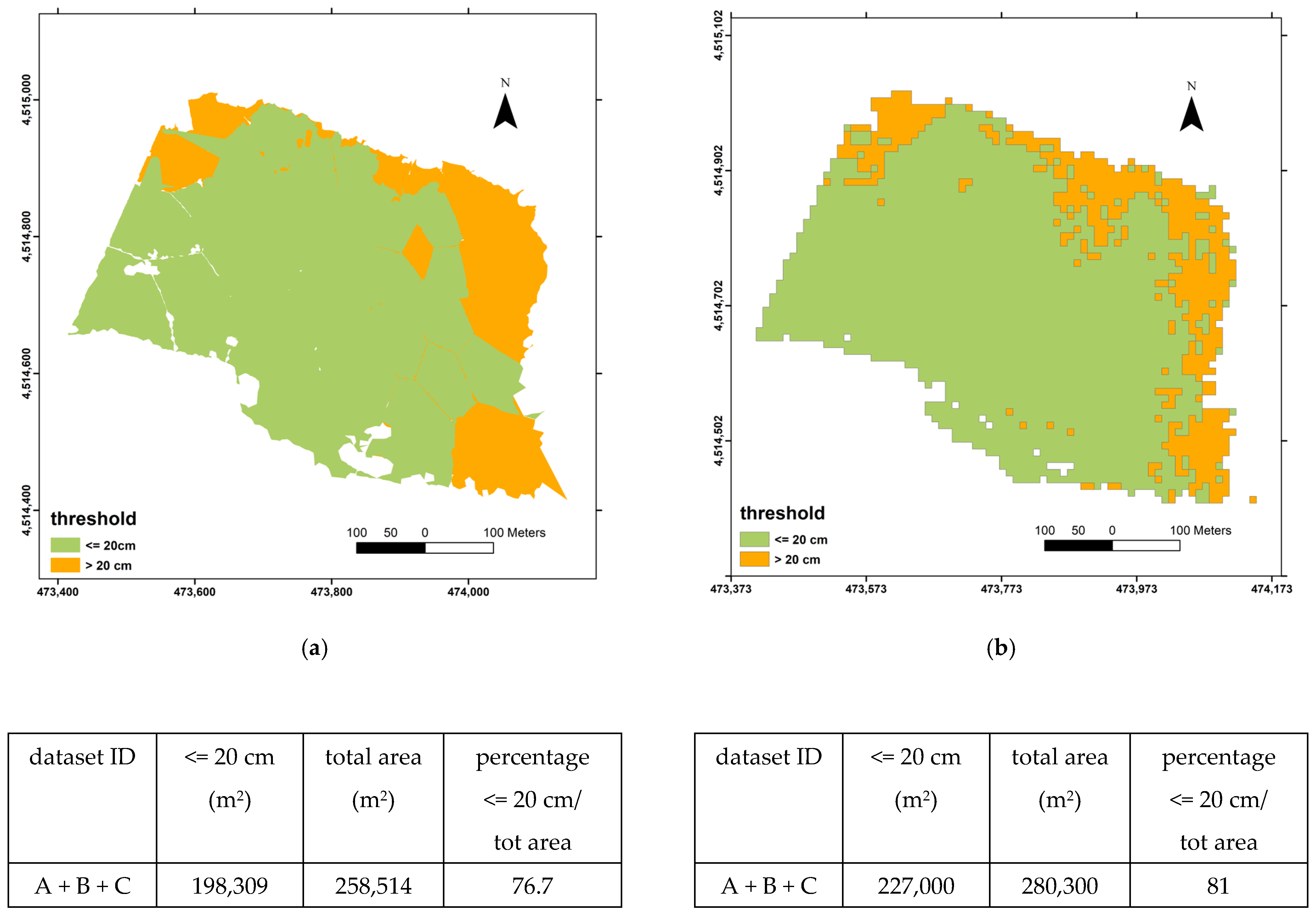
The three different TLS station positions allow different levels of area coverage at a given precision threshold (20 cm in Figure 12).

From the comparison of results in

Table 3. Area resulting from the dissolve of groups with mean error below the 20 cm threshold and percentage relative to the total area surveyed from each of the three stations.

Dataset 20.	≤20 cm (m2)	Total Area (m2)	Percentage ≤ 20 cm/Tot Area
A	126,539	204,929	61.7
B	96,938	234,115	41.4
C	81,463	137,655	59.0

, it can be concluded that the ideal station location is point A, while point B is the least appropriate in terms of coverage level. The simulation from point C covers a significantly smaller area than the others (about two-thirds), but it is the only one to present a group with mean error below 5 cm.

With 20 cm chosen as the target threshold, the merge and subsequent dissolve of the three stations can be performed to evaluate the area over which the target precision is achievable (Figure 13).

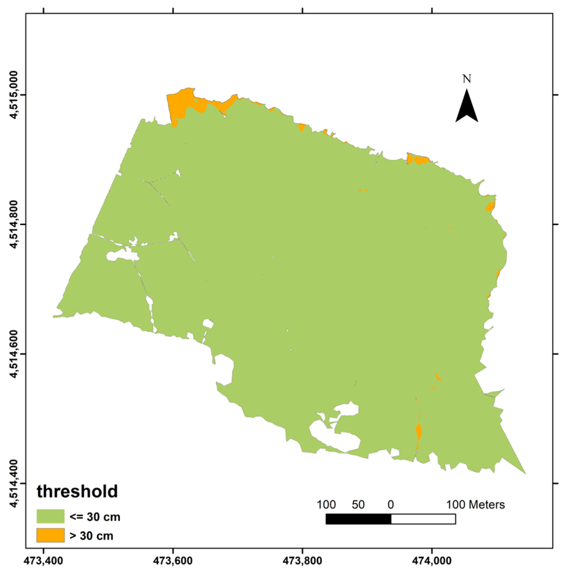
The simulation allows us to conclude that a mean error (ge) below 30 cm should not be expected across the entire scannable area.

As can be seen in Figure 14, by raising the threshold to 30 cm, practically the entire area covered by the three simulations would fall within it.

4.7. Focus on a Specific Area of Interest

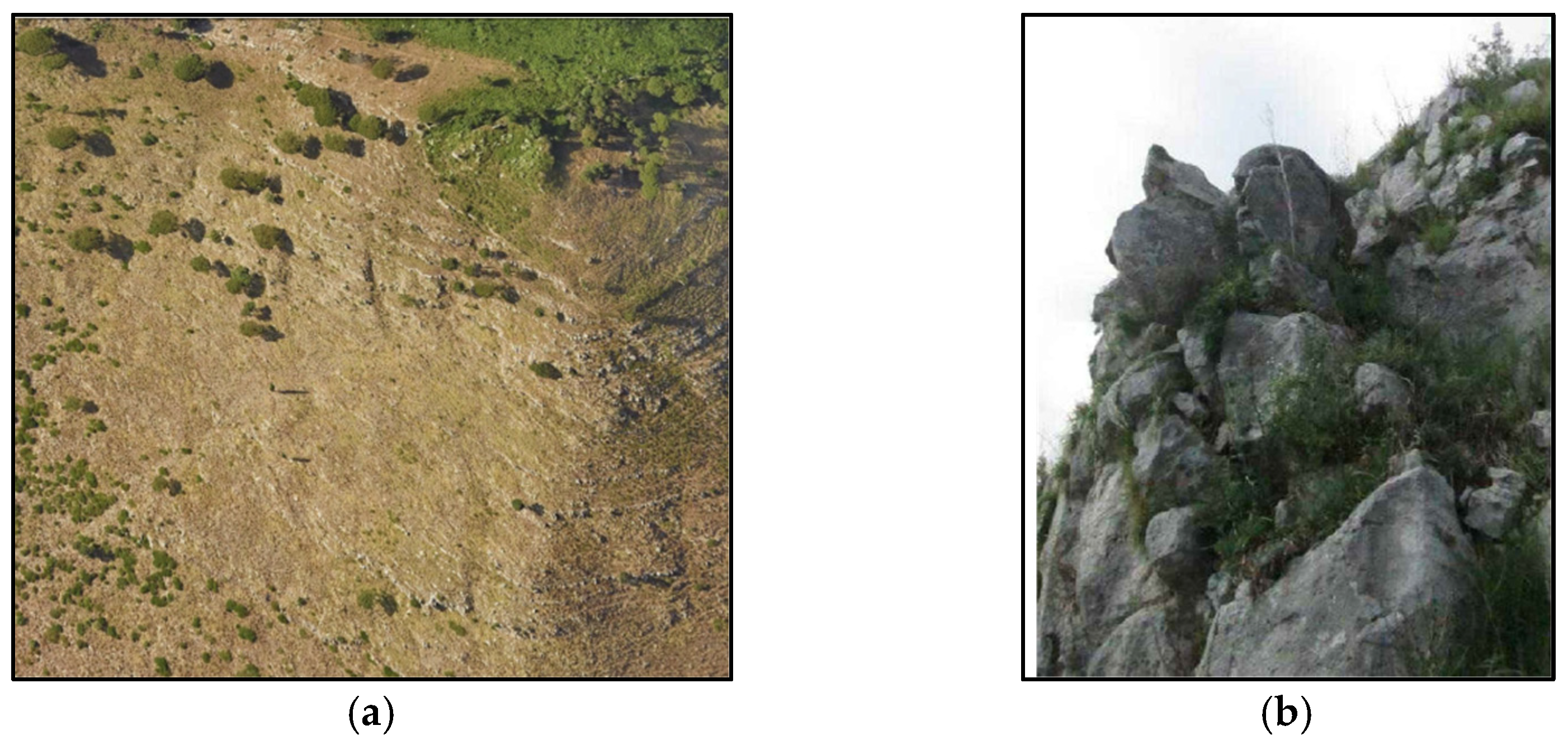
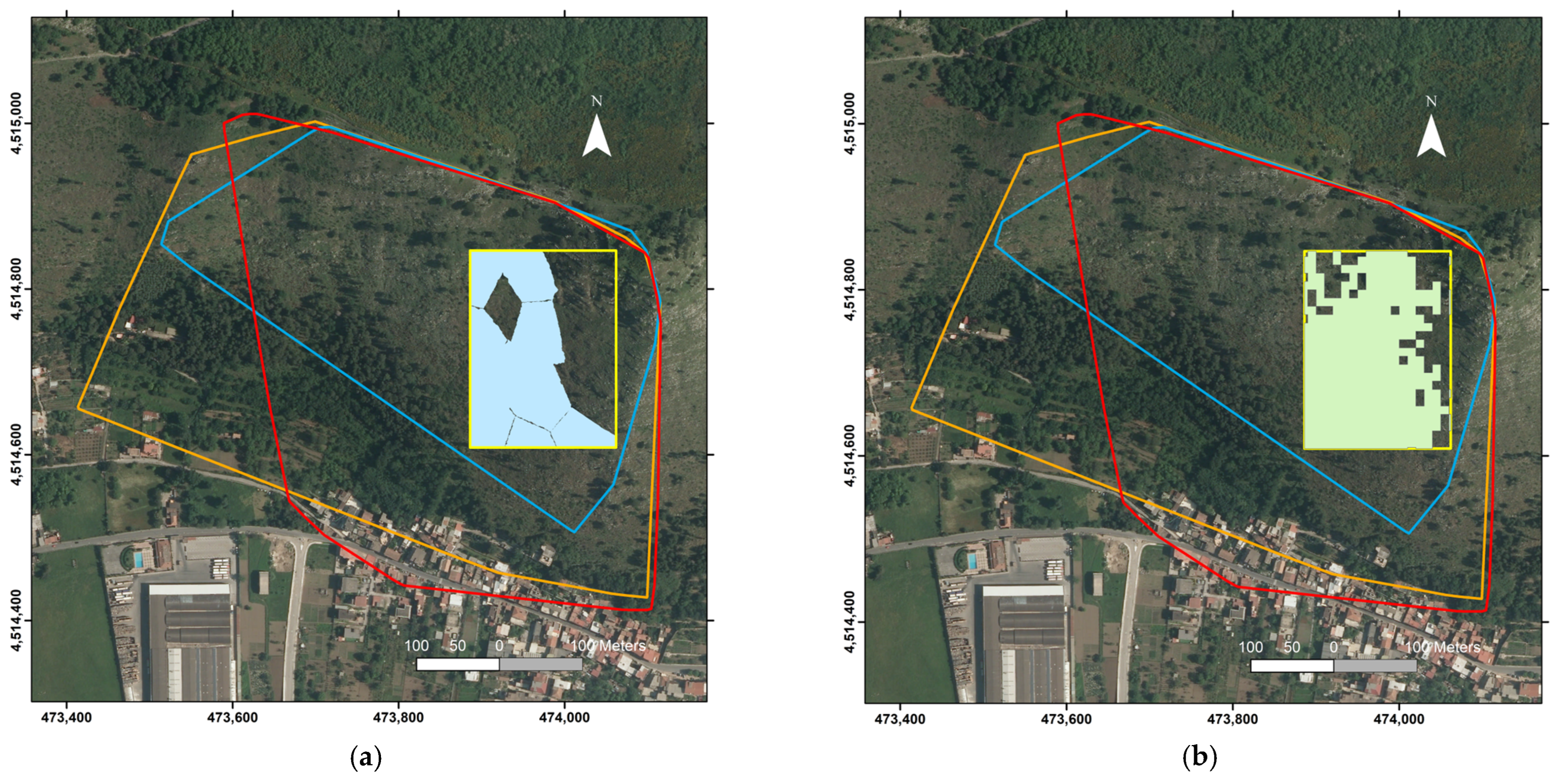
Beyond these general considerations, the appropriateness of carrying out the survey from one station point rather than another depends primarily on the location of the specific area intended to be surveyed with greater accuracy. For example, if we are interested in studying the rock outcrops considered susceptible to collapse, located in the northeastern portion of the slope [20] considered in the simulation, it is possible to further refine the analysis by defining a rectangular area of interest that encompasses them.

A comparison is then made between the simulations corresponding to three different station positions over this specific area, in order to identify which of them provides the best acquisition geometry (Figure 15). Conversely, the portion of the area that does not meet the desired accuracy from the “best” station is also identified, thereby indicating which part of the survey must be complemented by another station in order to cover the entire area. Considering a maximum allowable error threshold of 20 cm, even the merging of the areas is not sufficient.

The two approaches, KMNoNorm and AHG, show good agreement, covering similar portions of the area of interest (61% and 58%, respectively).

5. Discussion

The proposed methodology results from a series of algorithmic choices that were refined during the experimental phase, particularly concerning the definition of the feature vector and the selection of the clustering approach.

Regarding the construction of the aggregated variable, several morphometric descriptors—such as surface roughness or the terrain roughness index—were deliberately excluded. Although easily derived from the TIN, these parameters were found to be highly correlated with other variables already included in the model and did not provide additional meaningful information. Their inclusion would mainly have increased the computational burden without improving the clustering outcome.

During preliminary testing, multiple off-the-shelf algorithms were evaluated, including Random Forest and Support Vector Machine classifiers. However, it was concluded that K-means is the most appropriate choice for this type of problem, as the goal is to identify compact groups in a continuous numerical space rather than to perform supervised prediction.

Consistent with recommendations in the literature, an effective use of K-means requires appropriate data preprocessing to reduce the impact of variable correlations and scale differences—typically through standardization or weighting—and, where beneficial, dimensionality reduction through PCA. In the present case, the first two principal components explain approximately 95% of the total variance, while the first three exceed 99%. This metric provides a sound criterion for selecting the number of components to retain, especially considering that the computational cost associated with using two or three PCs is nearly identical.

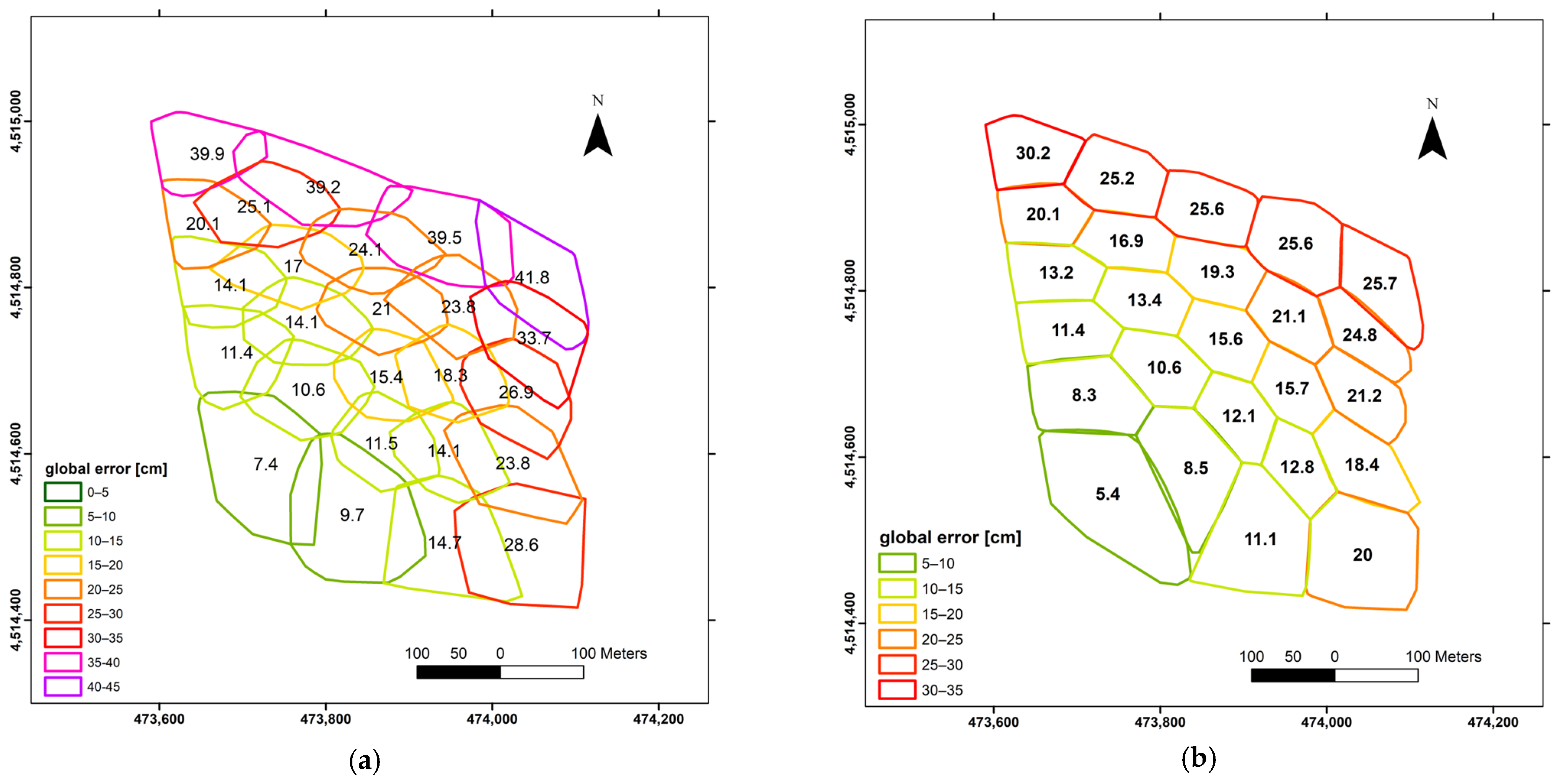
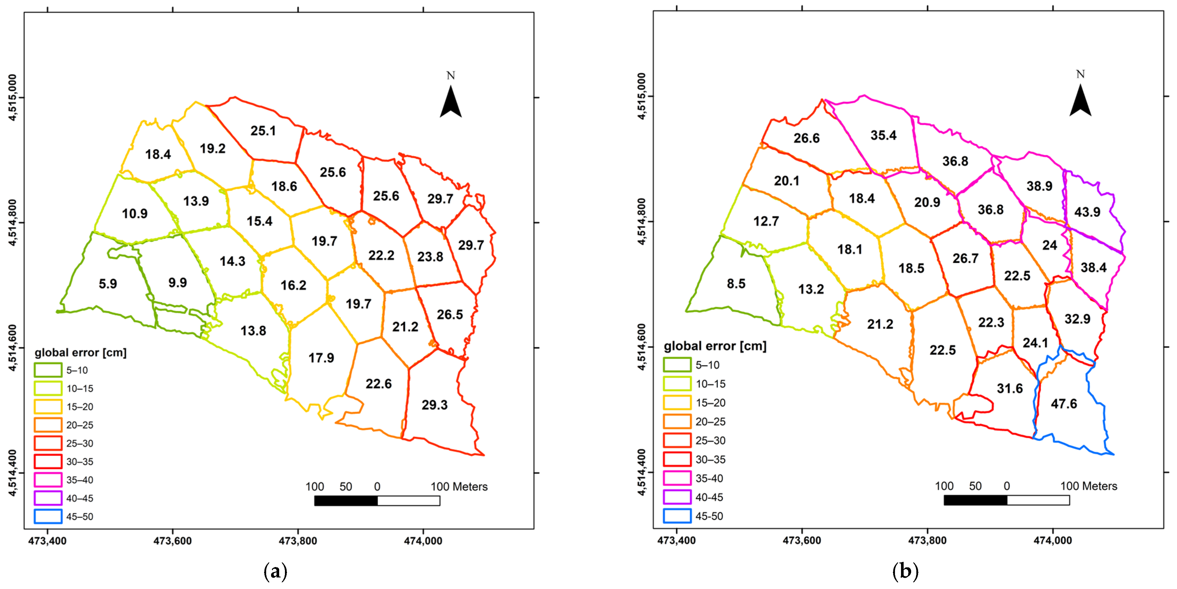
The KMNorm approach, which applies feature normalization prior to clustering, yielded less satisfactory results in the case study in terms of cluster separability and compactness. The resulting groups exhibit blurred boundaries and substantial spatial overlap. As shown in Figure 16, the convex hull polygons produced using KMNorm (a) display significant mutual overlap, whereas the polygons obtained with the KMNoNorm approach (b) are much more clearly separated.

From a quantitative standpoint, the extent of overlap can be assessed using an index such as Intersection over Union (IoU) or, more simply, by summing the overlapping areas. In our analysis, KMNorm produced a total overlap of 108,183 m², compared to only 4425 m² for KMNoNorm.

Similar considerations—although with different magnitudes—apply when adopting alternative boundary-estimation techniques, such as the concave hull [29,30].

This discrepancy arises because clustering quality indices (Silhouette, Davies–Bouldin, Calinski–Harabasz) evaluate compactness and separability in feature space, but they do not necessarily reflect the spatial coherence of clusters in the actual terrain coordinate system.

For this reason, the KMNoNorm approach, although statistically less orthodox, proved more effective in this case study in producing compact clusters with limited mutual overlap. The use of a rounded weight value of 100—equivalent to expressing ge in centimeters—was adopted as a practical choice to preserve an appropriate balance among variables while keeping the workflow simple.

Two approaches were examined for dimensionality reduction: PCA and UMAP. Both methods are sensitive to the scaling of input variables—PCA because principal components depend on variance, and UMAP because scaling affects the construction of the neighborhood graph and the resulting distortion of the low-dimensional embedding.

Experimental results showed that PCA provided better overall performance for this application, despite the nonlinear nature of the error model and of the relationships among variables—conditions under which UMAP would theoretically be more suitable.

The evaluation was carried out through both quantitative comparison of clustering quality indices and qualitative assessment of spatial cluster distribution in a GIS environment.

Qualitative analyses specifically focused on the correspondence between cluster boundaries and significant variations in incidence angle and key geomorphometric parameters (slope, aspect) and on the spatial separability of the groups, following a procedure analogous to that illustrated in Figure 16a.

Within the KMeansNorm framework, two standardization strategies were tested, each based on different measures of central tendency and dispersion, Standard Scaler (mean and standard deviation) and Robust Scaler (median and interquartile range). The Robust Scaler was introduced to mitigate the influence of distribution tails, i.e., residual outliers still present after the initial filtering.

Table 4. Comparison of clustering quality indices computed for 25 clusters obtained using the KMNorm approach applied to the dataset from station A. Substantially similar results were obtained with the KMNoNorm approach. The prefix “red” indicates the reduced-dimensionality space (e.g., PCA-based), whereas “geo” refers to the original terrain coordinates (east and north). The letter “w” denotes the configurations in which spatial coordinates were weighted. The row highlighted in green corresponds to the configuration that jointly optimizes the three indices.

Approach	Red Silhouette	Red Calinski–Harabasz	Red Davies–Bouldin	Geo Silhouette	Geo Calinski–Harabasz	Geo Davies–Bouldin
PCA RobustScaler	0.326	208,923	0.800	−0.128	7469	14.972
PCA RobustScaler w	0.323	166,208	0.826	0.009	52,013	6.580
PCA StandardScaler	0.323	168,475	0.804	−0.127	17,137	3.924
PCA StandardScaler w	0.347	224,504	0.797	0.265	197,042	0.957
UMAP StandardScaler	0.350	237,090	0.800	0.097	98,468	1.803
UMAP StandardScaler w	0.368	277,254	0.786	0.234	175,400	1.051
UMAP RobustScaler	0.355	235,876	0.782	−0.106	26,959	4.861
UMAP RobustScaler w	0.357	251,957	0.790	0.118	98,388	2.027

summarizes the comparison of clustering quality indices obtained using the KMeansNorm approach under the different dimensionality-reduction, scaling, and weighting configurations.

Since clustering was performed with fixed initialization parameters and evaluated on the entire dataset, the reported indices represent deterministic comparative metrics rather than statistical estimators.

Consequently, no estimator variance or variance propagation can be defined for these values, and the indices should therefore be interpreted as describing the behavior of the different methodological configurations rather than as statistical estimators intended for inferential testing.

It is worth noting that the indices computed in the reduced feature space are consistently better than those obtained in the terrain-coordinate space.

The better performance of PCA over UMAP in this context can be explained by the intrinsic geometric structure of the error model and its interaction with the Euclidean distance assumptions underlying K-means clustering.

Although the underlying error model exhibits nonlinear behavior (most notably the hyperbolic relationship between incidence angle and positional uncertainty) the dominant structure of the feature space can be regarded as being governed by spatial gradients and strongly correlated monotonic dependencies among the variables.

In particular, the positional error ge increases almost monotonically with the incidence angle (under the adopted filtering thresholds), while both incidence angle and distance are spatially structured by terrain morphology. As a consequence, these dependencies induce a strong spatial organization in the feature space, and the variability of the dataset is largely concentrated along a few dominant directions rather than distributed over a complex nonlinear manifold.

The incidence angle may nonetheless exhibit substantial local fluctuations, particularly in areas with overhanging rocks and morphological discontinuities, introducing local geometric heterogeneity in the feature space. However, these local variations do not generate intrinsic manifold complexity in the sense of folded, intertwined, or intrinsically nonlinearly separable structures and therefore the dataset maintains a globally ordered organization dominated by spatial gradients.

Under these conditions, PCA remains highly effective since the first principal component captures the dominant variance direction, largely driven by the high variance of incidence angle and its strong correlation with positional uncertainty. The linear projection preserves global metric relationships and supports spatial coherence in the reduced space.

In contrast, UMAP is designed to preserve local neighborhood topology and is particularly advantageous in the presence of topologically complex manifolds, while it may alter global distance relationships. From a clustering perspective, this distinction is critical since the K-means relies on Euclidean distance and benefits from embeddings that preserve global metric consistency.

Dimensionality reduction methods that preserve global distance relationships tend to provide more stable clustering results than approaches primarily designed to preserve local topology.

This explains why PCA yields clusters that are more spatially coherent and geomorphologically interpretable than those obtained through UMAP.

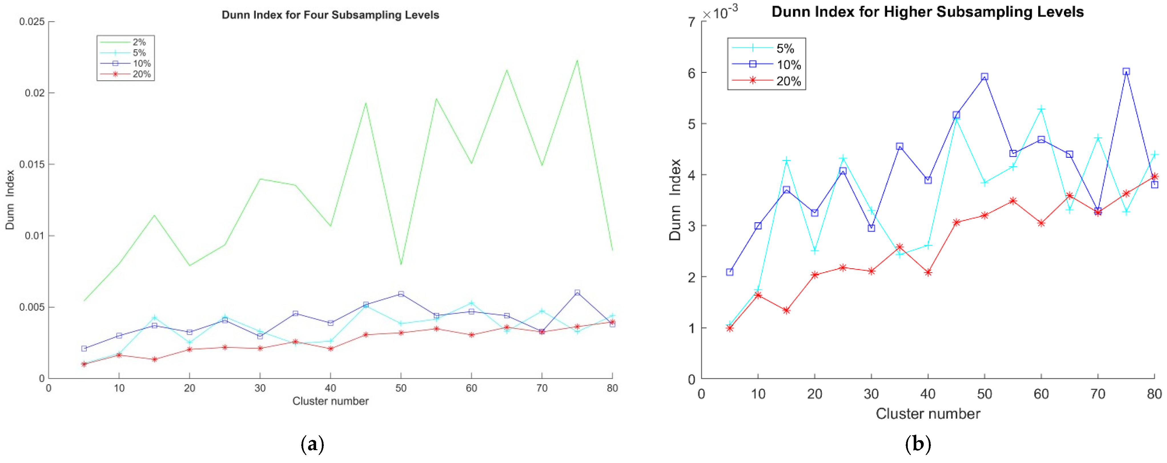
The Dunn Index was not included in the Results section, even though it is one of the most suitable indicators for evaluating cluster separability. Its computation on the full dataset—over 200,000 points in this case—is extremely demanding in terms of both memory requirements and processing time.

The use of a subsample is therefore necessary, although this introduces a limitation: excessively small samples may produce biased evaluations that depend more on sample size than on the intrinsic data structure.

Figure 17 shows the Dunn Index computed for subsamples of different sizes: 2%, 5%, 10%, and 20% of the full dataset, corresponding to approximately 2k, 10k, 20k, and 40k points, respectively.

For sample sizes of 5% or greater, the choice k = 25 is consistently supported, in agreement with the other cluster-quality indices. More generally, the Dunn Index shows an increasing trend with the number of clusters.

It is important to emphasize that this result should not be interpreted as a general guideline: the appropriate sample size depends on the user’s computational resources and on the specific characteristics of the dataset.

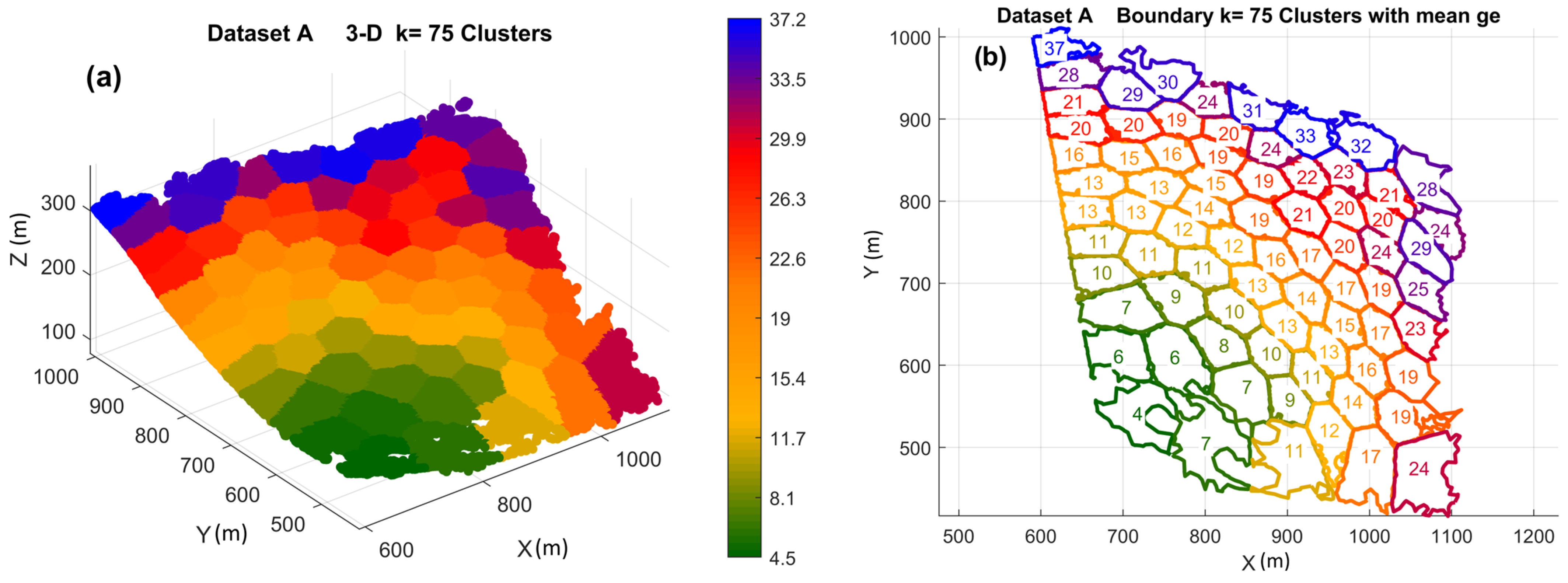
The number of clusters used as input for the K-means algorithm was determined through a comparative analysis of clustering quality indices. However, if a higher level of detail is preferred, increasing the number of clusters entails only a marginal computational overhead.

Figure 18 illustrates the clustering results for k = 75. The increased spatial detail can be appreciated by comparing this figure with the corresponding Figure 8.

In the KMNoNorm configuration, the error parameter ge was multiplied by a factor of 100 in order to express the error in centimeters rather than meters. This scaling step aligns the numerical magnitude of the error component with that of the spatial coordinates, which are expressed in meters, and therefore prevents the error variable from being numerically underrepresented within the variance-based PCA framework.

This scaling factor is not related to the specific morphology of the study area but rather to the order of magnitude of the quantities typically involved in TLS surveys. In practice, the spatial extent of the scanned area is generally of the order of hundreds of meters, whereas the expected measurement error is typically expressed in centimeters. For this reason, expressing the error in centimeters represents a practical normalization that is broadly applicable across typical TLS survey configurations.

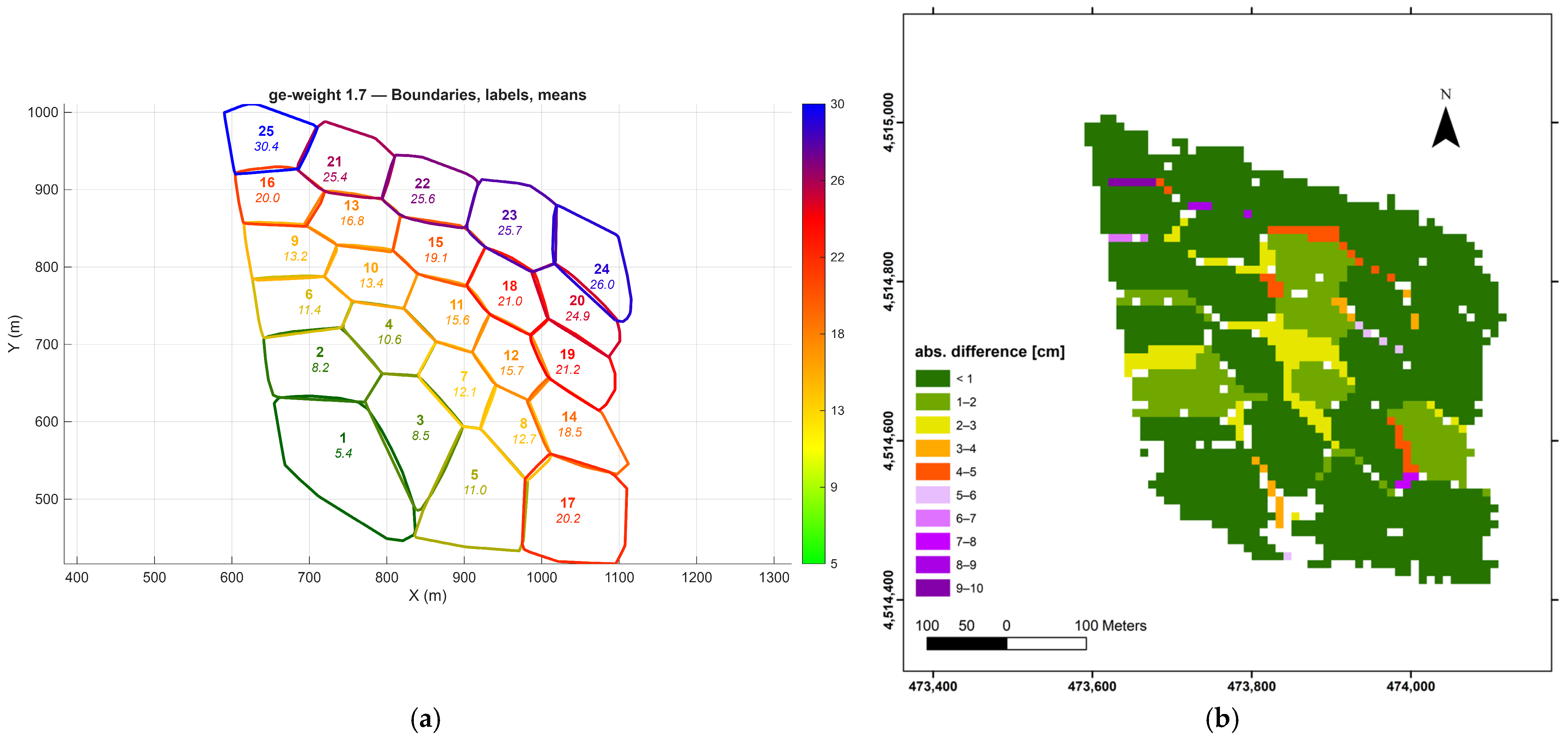
For the present case study, the ratio between the variable ranges would suggest an additional weighting factor of approximately 1.7. A sensitivity check was therefore performed by comparing the clustering results obtained using scaling factors of 100 and 170. The configuration obtained with the factor 170 is illustrated in Figure 19a.

To perform a consistent comparison between the two configurations, the cluster mean errors were evaluated at the nodes of a regular vector grid with 10 m spacing. Through a spatial join, each grid node was associated with the mean error of the cluster obtained under the two weighting schemes (100 and 170), allowing the computation of absolute differences between the two realizations.

The comparison shows that the differences remain limited: 75.5% of the absolute differences in cluster mean error are below 1 cm, 96.4% are below 3 cm, and 98.9% are below 5 cm, while only 1.1% exceed 5 cm. The spatial distribution of these differences is shown in Figure 19b.

Furthermore, no appreciable differences were observed in the spatial configuration of the clusters or in their separability in feature space. These results indicate that the clustering outcomes are largely insensitive to moderate variations in the scaling of the error parameter.

Figure 12 and Figure 13 suggest that the AHG approach provides a larger area meeting the 20-cm error threshold compared to the KMNoNorm method. However, it should be noted that AHG relies solely on the global error ge, whereas KMNoNorm clusters a more complex variable that explicitly incorporates TIN morphology. As a result, the two approaches are not directly comparable in quantitative terms.

It should also be noted that applying more restrictive filtering thresholds reduces the number of retained points while simultaneously reducing the mean error associated with each group, as shown in Figure 20.

Consequently, regardless of the chosen aggregation approach, stricter filtering thresholds tend to increase the proportion of retained observations that satisfy a given precision requirement, while reducing overall point density.

The resulting spatial representation of high-precision zones may therefore appear more continuous or more extensive; however, this effect is conditioned by local sampling density and does not alter the underlying geomorphological structure that governs uncertainty distribution.

Ultimately, the balance between these parameters depends on the scale at which the laser-scanner-derived products are intended to be used and displayed, as the representation scale is inherently constrained by point density [31].

6. Conclusions

This work presents an innovative procedure for the a priori assessment of TLS survey accuracy on landslide slopes by integrating a physically motivated error model with high-resolution spatial aggregation based on unsupervised clustering. The proposed workflow can be applied using different TLS error models, provided it accounts for the key factors governing measurement uncertainty—beam divergence, range, and incidence angle.

So far, the focus of this study has been on the generalization of the error model, whereas the proposed workflow has been applied to a single test case. Nevertheless, the selected study area is considered representative of a relatively common landslide morphology.

Homogeneous-accuracy areas are identified by clustering a multidimensional feature vector that includes point coordinates, modeled positional error, incidence angle, and range. Before clustering, the feature space is reduced through PCA, which preserves the dominant geometric information while mitigating redundancy. K-means is then applied to delineate spatially coherent regions characterized by similar expected accuracy levels.

Results show that strong local variability in incidence angle generates sharp discontinuities in the simulated error field, making simple classification ineffective. In contrast, the clustering-based approach yields spatially consistent accuracy zones that more faithfully reflect morphological variations across the slope.

The proposed method supports TLS survey planning by enabling a quantitative comparison of alternative stationing configurations, identifying areas that can be acquired within a given accuracy threshold, and highlighting zones where additional scans are required.

The stationing positions assumed in the simulation can be easily materialized in the field using standard GNSS techniques.

The procedure requires an initial topographic model of the slope, and its performance—both in terms of reliability and computational load—depends on the geometric characteristics of the TIN. Determining an optimal number of clusters remains non-trivial, and an important open challenge is the efficient integration of simulation results obtained from multiple TLS stations.

Finally, the framework designed for a priori station optimization can also be applied a posteriori. By using the actual scanner position measured in the field and deriving a simplified TIN from the acquired point cloud, the method allows reconstruction of the accuracy actually achieved across the slope, according to the adopted error model; of course, defining a truly realistic error model is the hard part.