Article

Evaluating Machine Learning and Statistical Prediction Techniques in Margin Sampling Active Learning for Rapid Landslide Mapping

1
Space Star Technology Co., Ltd., Beijing 100086, China
2
Department of Land, Air, and Water Resource, University of California at Davis, Davis, CA 95616, USA
3
Laboratory of Artificial Intelligence, Hangzhou Institute of Technology, Xidian University, Hangzhou 311231, China
4
Technology and Engineering Center for Space Utilization, Chinese Academy of Sciences, Beijing 100094, China
5
Beijing Key Laboratory of Precision Forestry, Beijing Forestry University, Beijing 100083, China
*
Author to whom correspondence should be addressed.
Geomatics 2025, 5(4), 74; https://doi.org/10.3390/geomatics5040074 (registering DOI)
Submission received: 7 October 2025 / Revised: 21 November 2025 / Accepted: 27 November 2025 / Published: 2 December 2025

Abstract

Rapid and accurate landslide detection is important for minimizing loss of life and property. Supervised machine learning has shown promise for automating landslide mapping, but it often requires thousands of labeled instances, which is impractical for timely emergency responses. Margin sampling active learning (MS) has proven effective for rapid landslide mapping by querying the most “informative” instances. However, it is still unclear how the choice of the landslide modeling algorithm influences the effectiveness of MS. This study assessed MS with four common landslide modeling algorithms, i.e., random forest, support vector machine, a generalized additive model, and an artificial neural network, using an open-source landslide inventory from Iburi, Japan. The results showed that all four combinations obtained > 0.90 the area under the ROC curve (AUROC) with 150 to 400 training instances. In particular, MS integrated with random forest performed best overall, with a mean AUROC of 0.91 and correct delineation of about 60 percent of the mapped landslide area using only 150 training instances. Precision-recall analysis within the ranked susceptibility maps showed that MS integrated with random forest and support vector machine generally outperformed the generalized additive model and artificial neural network. In addition, we developed a graphical user interface using R Shiny that integrates the MS active learning workflow with all four modeling options. Overall, these findings advance machine learning in rapid hazard mapping and provide tools to support decision-makers in emergency response.

1. Introduction

As one of the most devastating natural hazards worldwide, landslides cause severe economic losses, infrastructure damage, and loss of human life. For example, from January 2004 to December 2016, a total of 55,997 people were killed in 4862 distinct landslide events [1]. Therefore, rapid detection and early warning are necessary not only for immediate emergency response but also for long-term risk management and planning. Machine learning has shown usefulness for the automated detection of landslides, especially supervised machine learning algorithms [2]. However, Ref. [3] have pointed out that supervised machine learning algorithms require a sufficient number of training instances, especially in pixel-based landslide detection.
Recent advances in remote sensing technology have greatly enhanced our ability to observe and monitor Earth surface processes. For example, Ref. [4] achieved automatic slow-moving landslides detection over a large area by combining Synthetic Aperture Radar Interferometry with machine learning. The authors of [5] have demonstrated that Unmanned Aerial Vehicles allow for rapid and easy data acquisition, enhancing the capabilities of landslide detection. The authors of [6] provided a systematic review of spaceborne InSAR in landslide monitoring and susceptibility mapping. The authors of [7] illustrated practical applications of remote sensing in monitoring active landslides, thereby giving readers a concrete example of recent research. The authors of [8] summarized how Synthetic Aperture Radar and optical methods have rapidly advanced landslide failure detection. However, regardless of data quality and sensor calibration, the practical implementation of these technologies in landslide detection is hampered by the challenge related to data labeling. As [9] has pointed out, landslide occurrences are rare compared to the vast areas of stable terrain, resulting in the high cost and labor-intensive process of manual annotation in order to obtain enough training instances. In this way, even when high-quality remote sensing data is available, the efficiency of many supervised algorithms is reduced, ultimately impacting the effectiveness of emergency rescue operations.
To address this challenge, active learning has emerged as a promising solution aimed at achieving high predictive accuracy with a small number of training instances [10]. It strategically selects the most “informative” instances that are most likely to improve model performance, thereby reducing the need for extensive manual annotation while maintaining robust results [11]. Among various active learning strategies, margin sampling (MS) has shown its effectiveness in landslide hazard assessments by selecting a small number of “informative” instances. For example, Ref. [12] showed that MS outperformed other active learning strategies in pixel-based landslide detection assessments in Ecuador by combining with the support vector machines (SVM). The authors of [13] achieved unsupervised landslide detection by combining MS and transfer learning based on the generalized additive models (GAM). Despite the promising results of MS, these studies have indicated that its effectiveness might vary depending on the supervised algorithm used.
In addition, recent comparative studies have indicated that different models handle training data in different ways, resulting in different predictive performances [14]. Yet no single best landslide susceptibility/detection modeling algorithm has been identified. For example, Ref. [15] indicated that the random forest (RF) had the overall best predictive performance by comparing multiple models, including GAM and SVM, in three areas in the province of Lower Austria, Austria. The authors of [16] demonstrated that SVM outperformed the Artificial Neural Network (ANN), RF, and logistic regression with a small number of training instances by reviewing past studies. The authors of [17] displayed that ANN had a higher prediction capability than SVM, logistic regression, and logistic model trees in a shallow landslide hazard assessment. The authors of [18] concluded that the GAM outperformed the generalized linear model in estimating the probability of shallow landslide occurrence. The authors of [14] have shown that while deep learning methods are more accurate than traditional machine learning approaches when data is abundant, landslide hazard assessments normally lack sufficient data to fully train deep learning networks.
Therefore, considering no single algorithm is effective in all scenarios (e.g., different study areas) in landslide hazard assessments [14,16], and no studies have systematically examined whether different modeling algorithms affect active learning outcomes in landslide mapping, this study aims to evaluate the robustness of MS across four widely used landslide modeling algorithms (i.e., GAM, SVM, RF, and ANN). In addition, to make MS more practical, we developed a graphical user interface (GUI) by integrating MS with the above algorithms, thereby enabling the interactive selection of “informative” training instances for different applications. This GUI enables users to upload their own datasets, choose the desired modeling technique, specify the number of “informative” instances they wish to label, and then receive these selected instances for further annotation.

2. Data

2.1. Study Area

The study area was defined based on the boundaries established by [19] in the eastern and central Iburi regions of Hokkaido, Northern Japan, with modifications to account for cloud cover in the remote sensing data (Figure 1). It features numerous active faults (e.g., segments of the Eastern Boundary Fault Zone) and comprises diverse lithological units dominated by Neogene to Quaternary sedimentary rocks and Late Pleistocene non-alkaline pyroclastic deposits, with topographic variability ranging from rugged, high-elevation terrains in the east to hilly and lowland areas in the central and western parts. In 2018, the study area suffered intense ground shaking that was caused by the earthquake with Mj 6.7/Mw 6.6, resulting in 5625 identified co-seismic landslides over 46.3 km2. These landslides are primarily characterized by translational movements with shallow sliding surfaces and long run-out distances.

2.2. Pixel-Based Landslide Inventory

The landslides in this analysis are a subset of an inventory for the Iburi region that has been previously published by [19]. The full inventory comprises 5625 individual landslide polygons covering 46.3 km2. Initially, a database containing 3307 landslide polygons was mapped within days after the mainshock by the Geospatial Information Authority of Japan. Subsequent manual segmentation and aggregation, which were based on valley lines, ridge lines, the hillshade, and the slope aspect derived from a 10 m resolution DEM and high-resolution aerial imagery, refined this database. Further details on the landslide inventory and its quality can be found in [19]. For our analysis, 5491 landslides were extracted from the inventory to build the pixel-based landslide inventory, after excluding polygons that were partially or fully obscured by cloud cover in the remote sensing imagery.
First, the Minimum Mapping Unit was applied for removing the landslide polygons that are smaller than 400 m2 for Digital Elevation Models (DEMs) with a 10 m × 10 m resolution provided by the Geospatial Information Authority of Japan [20], resulting in 5473 landslide polygons. Next, a 200 m buffer was generated around these landslide polygons. Finally, landslide points/instances were randomly sampled within the landslide polygons, and non-landslide points/instances were randomly sampled from areas outside 200 m buffer areas, yielding 385,329 landslide points/instances and about 9.73 million non-landslide points/instances.

2.3. Predictor Variables

Topographic analysis commonly forms the basis of quantitative landslide modeling [21,22,23]. Previous studies have demonstrated that topographic attributes derived from elevation models serve as effective proxies for surface processes and geophysical site conditions, thereby simplifying complex geomorphological relationships [24,25]. In this study, predictor variables were derived from a 10 m × 10 m digital elevation model (DEM) and pre- and post-event optical imagery. The local slope angle (°, slope), elevation (m, dem), plan and profile curvature (rad m−1, plancurv, and profcurv), catchment slope angle (cslope), SAGA Topographic Wetness Index (SWI), and upslope contributing area (m2), which have been widely used as proxies for destabilizing forces, water availability, and wind exposure, were selected as topographic variables in this study [12,26]. In addition to the topographic attributes, the difference between the normalized difference vegetation index (NDVI) of pre- and post-event PlanetScope optical images was included, which can effectively distinguish green vegetation from landslide-affected areas [27,28]. All predictor variables were generated using the R package “RSAGA” and processed in SAGA GIS 7.4.0, and all variables that presented outliers were winsorized at the 1st and 99th percentiles. Table 1 provides a summary of the predictor variables used for both landslide and non-landslide instances.

3. Methods

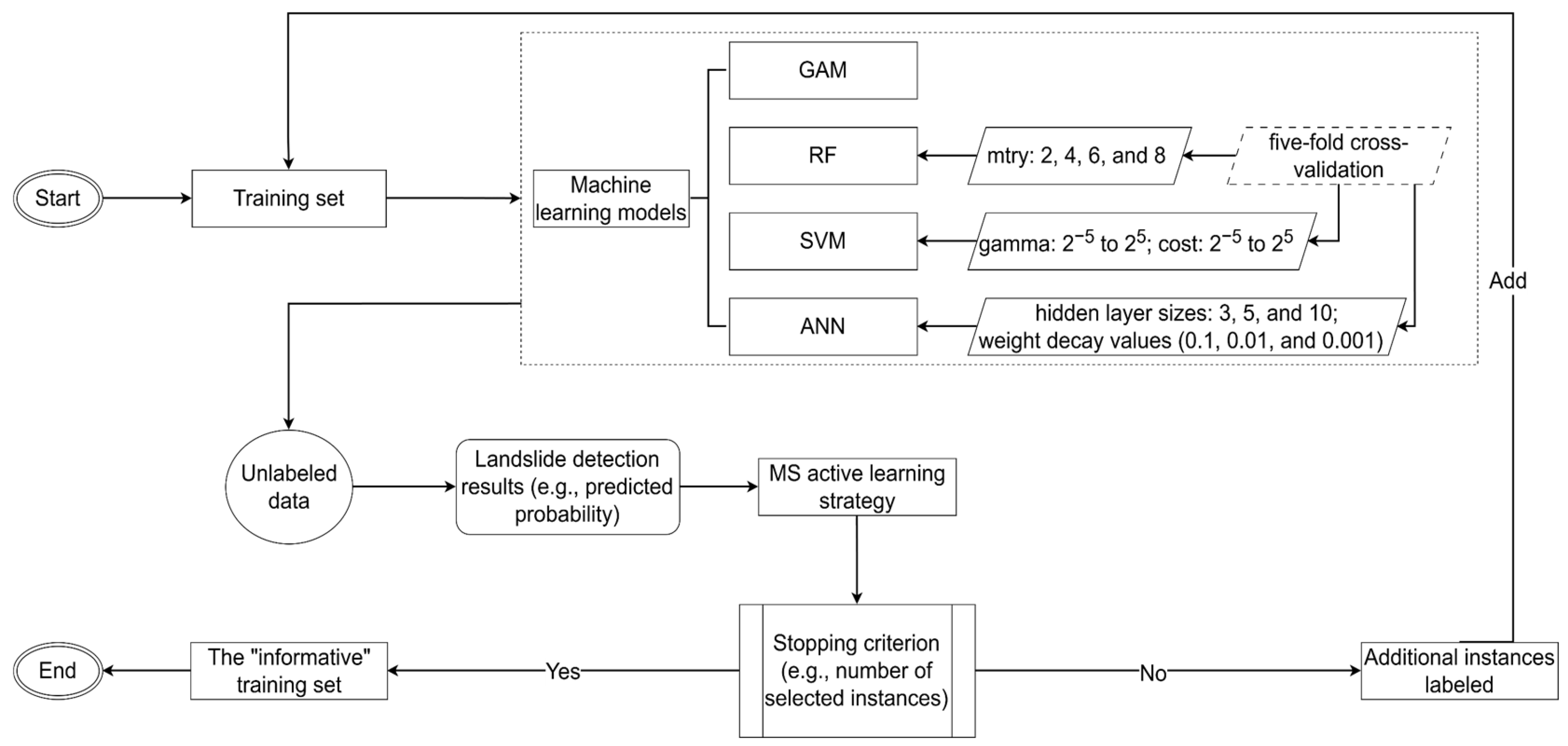
In this study, we integrated GAM, RF, SVM, and ANN into a margin sampling active learning workflow to investigate their impacts on the performance of MS in landslide detection assessments (Figure 2). We began with a small initial training set and fit four machine learning models for landslide prediction. The best-tuned model is then applied to the unlabeled data to obtain predicted probabilities. The margin sampling strategy evaluated these probabilities and selected the most "informative" additional instances, which were then labeled and added to the training set. This loop of model fitting, prediction, and instance selection continued until a predefined stopping criterion based on the number of selected instances was met, yielding the final informative training set used in the final landslide detection results.

3.1. Landslide Modeling Techniques

Four statistical and machine learning techniques are compared in this study: the generalized additive model with stepwise variable selection (GAM; [29]), the support vector machine (SVM; [30]), random forest (RF; [31]), the artificial neural network (ANN, [32]). Because rapid landslide detection is one of our primary objectives, we selected configurations that avoid unnecessary training delays and are considered typical for most applications.
GAM is a flexible statistical approach that captures nonlinear relationships between the response and predictor variables through the use of smooth functions [33]. It can effectively accommodate the complex and nonlinear geomorphological processes underlying landslides without the need for extensive manual tuning [26]. In our study, the R package “mgcv” was applied to achieve the GAM with smooth splines and default smoothing parameter estimation [34].
SVM is a robust machine learning technique that operates by mapping predictors into a high-dimensional feature space through nonlinear transformations, where a decision hyperplane is established to separate classes [35]. Previous studies have proven its effectiveness in landslide hazard assessments due to its capacity to capture complex, nonlinear relationships among geomorphological variables [36,37]. In our study, the implementation of SVM with a radial basis function kernel used the “caret” package in R [38]. The model was trained on the predictors mentioned above through five-fold cross-validation. The parameter tuning was conducted over a range of regularization parameters from 2−5 to 25 and kernel bandwidths from 2−5 to 25 under a grid search.
RF is an ensemble machine learning technique that constructs numerous decision trees and aggregates their predictions to enhance classification performance [39]. Due to its capability in modeling complex, nonlinear interactions among predictors, it is widely used in landslide hazard assessments [40]. In our study, we implemented RF using the “caret” R package with five-fold cross-validation employed [38]. A grid search was performed to optimize the number of variables randomly sampled at each split (mtry), testing candidate values of 2, 4, 6, and 8, while 500 trees were grown in each forest.
ANN is a machine learning technique modeled after the brain’s network of interconnected neurons, enabling it to capture and represent complex, nonlinear relationships among predictors [41]. The input data is processed through one or more hidden layers before reaching the output layer, thereby capturing intricate patterns in the data. Previous research has demonstrated the usefulness of ANN in landslide hazard assessments [42,43]. The ANN used in our study was achieved by using the "nnet" method from the R package “caret” [38]. The parameter tuning was conducted via a grid search over hidden layer sizes (with candidate values of 3, 5, and 10 neurons) and weight decay values (0.1, 0.01, and 0.001) using five-fold cross-validation.

3.2. Margin Sampling Active Learning

Margin sampling active learning (MS) is an efficient strategy for reducing annotation costs while enhancing model performance by focusing on selecting the most “informative” unlabeled instances [12]. It is to quantify the information (i.e., uncertainty) for each instance by examining the difference between the posterior probabilities of the two most likely classes. In our study, for each unlabeled landslide/non-landslide instance x , the “informative” landslide/non-landslide instance is defined as:
x m s = a r g   min x P θ y 1 * x P θ y 2 * x ,
where P θ y x represents the posterior probability of class y (i.e., landslide or non-landslide) for the unlabeled landslide/non-landslide x , as predicted by the model described above θ . A smaller difference means that the classifier is less certain about its class, implying that obtaining the true class for such landslide/non-landslide instance is most likely to obtain valuable information to refine the decision boundary.

3.3. Experiment Design and Performance Evaluation

In our experiments, we initially selected a training set of 100 instances to approximate the spatial distribution of landslides in the study area, with approximately 90% non-landslide and 10% landslide instances. Each of the models (i.e., SVM, RF, ANN, GAM) was first trained on this initial dataset and then used to predict the labels for the remaining unlabeled instances. Subsequently, we applied the MS active learning to select the most “informative” instances based on the predictive probability. In each iteration/epoch, an additional 25 instances were queried and incorporated into the training set. This iterative process was repeated for 50 epochs in order to observe the convergence of results for large instance sizes (1350 labeled instances), though such instance sizes may be impractical in operational settings. To mitigate the influence of random variability, the entire experiment was repeated 100 times.
The performance of each combination was evaluated using the area under the receiver operating characteristic (ROC) curve (AUROC), which ranges from 0.5 (indicating no predictive skill) to 1 (indicating perfect classification) [43,44,45] and produced landslide detection maps. To better characterize model behavior under pronounced class imbalance, precision and recall were evaluated in the top 1, 2, 4, 5, and 10 % of ranked susceptibility values, which quantify, respectively, the fraction of correctly identified landslide pixels and the proportion of the mapped landslide inventory captured within a given proportion of the study area. In addition, a permutation-based variable accuracy importance approach was applied to assess variable importance across all combinations by computing how much a performance measure reduces when each variable is randomly permuted [46]. Following [47], the variable importance of each combination was measured by calculating the change in median AUROC values estimated by spatial cross-validation. Each variable was permuted ten times for each test fold for a total of 50 permutations per variable, and the AUROC of the prediction for each permutation was measured and compared to the unperturbed predictive performance. The variable importance was standardized for each combination by using a min–max scaling procedure for an individual variable, yielding normalized importance scores ranging from 0 (low relative importance) to 1 (high relative importance).

3.4. Graphical User Interface

The graphical user interface (GUI) was developed in R version 4.3.2 using the Shiny framework, which allows users to do data upload, model configuration, iterative training, uncertainty sampling, label editing, and model updating (Figure 3). A logical sequence of steps is designed to iteratively select “informative” instances:
Upload Data: Users upload an initial labeled training dataset and an unlabeled dataset in .csv format, which must contain (x, y) coordinates. The training dataset should also have a “label” column with 1 for landslide and 0 for non-landslide. The uploaded training dataset and unlabeled dataset will be previewed under “Training Data Preview” and “Unlabeled Data Preview”, respectively.
Choose Model and Parameters: Users can select one of four models (i.e., SVM, RF, ANN, or GAM) by using a drop-down menu. Users can specify the number of cross-validation folds, how many repeats to include, and the tuning complexity. These are helpful in hyperparameter tuning. By clicking “Train Model”, the performance metrics of the selected model and predicted probability for each unlabeled instance in landslide and non-landslide are generated, which will show under “Model Training Results” and “Unlabeled Data Predictions”, respectively.
Active Learning: Users can define how many additional instances they want to obtain. These instances are identified via the margin sampling active learning, and display under “Most Uncertain Samples (Editable)” by clicking “Select Uncertain Samples”.
Add New Labels: Users can directly edit the uncertain instances through an interactive table or upload a CSV containing newly labeled data by using “Upload Edited Uncertain Samples (CSV)”. Also, it allows users to upload a CSV containing other labeled instances by using “Upload Additional New Training Data (CSV)”, which will display under “Extra Selected Data Upload from CSV”. By clicking “Update Data”, the training dataset will be updated by integrating these additional instances and will show under “Updated Training Data Preview”. In addition, users can retrain the selected model based on the updated training dataset by clicking “Train model”.
Downloads: Users can export the updated training dataset in CSV format.

4. Results

4.1. Comparison of Predictive Accuracy

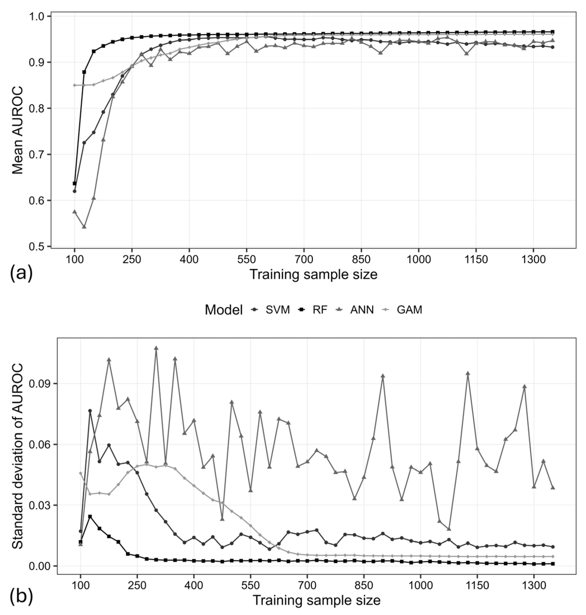
The comparison of model performance across training instance sizes revealed differences in the mean AUROC among combinations of MS with algorithms, in which MS integrated with RF had the overall best predictive accuracy, followed by MS integrated with SVM (Figure 4a). MS integrated with RF obtained the highest mean AUROC throughout the entire learning process and rapidly converged to a stable performance. Under 150 landslide and non-landslide instances, MS integrated with RF achieved a mean AUROC of 0.91, and its performance in the mean AUROC continued to improve, plateauing near 0.96 after approximately 400 total training instances (combining landslides and non-landslides). MS integrated with SVM had a similar performance in the mean AUROC, but it required a slightly larger training set (around 250 landslide and non-landslide instances) to achieve the comparable mean AUROC obtained by MS integrated with RF, with 150 total training instances. In contrast, MS integrated with both ANN and GAM showed lower mean AUROCs at small instance sizes and slower improvement in the mean AUROCs in the entire learning process. For example, with 150 total training instances, the mean AUROC obtained by MS integrated with ANN was lower than 0.75, and that obtained by MS integrated with GAM was around 0.83. All landslide models converged to relatively high mean AUROCs with more than 400 total training instances, and MS integrated with RF and SVM consistently outperformed MS integrated with ANN and GAM across almost all training instance sizes.
The standard deviation of AUROCs illustrated that MS integrated with RF and SVM showed lower variability compared to MS integrated with ANN and GAM, particularly when the number of training instances exceeded 300, which was consistent with the performance in the mean AUROC (Figure 4b). MS integrated with RF achieved the lowest standard deviation in the standard deviation of AUROCs across all training instance sizes, with variability dropping below 0.01 after only 200 total training instances. MS integrated with SVM also displayed a low variance in AUROCs over 100 repetitions, particularly beyond 300 total training instances. In contrast, MS integrated with ANN showed high variability in AUROCs across the entire learning process, with a standard deviation of AUROCs often exceeding 0.06 even when over 1000 total training instances were used. MS integrated with GAM displayed intermediate behavior, with moderate variability at small training instance sizes that gradually decreased as more training instances were added, ultimately stabilizing around 0.02.
Precision-recall metrics within the ranked susceptibility maps were consistent with these AUROC patterns (Table 2). For a training size of 150 instances, MS integrated with RF produced precision in the top 1 and 2% of the mapped areas around 0.90, whereas ANN, GAM, and SVM showed lower precision in the same fraction of area. As the number of training instances increased to 250 and 400, precision in the top 1 and 4% areas rose to approximately 0.80–0.90 for all models, and RF and SVM generally remained at the upper end of the precision range across area fractions. In terms of recall at fixed area fractions, all models captured about 0.04–0.05 of the total inventoried landslide area within the top 1% of areas and approximately 0.40–0.42 within the top 10% area, again with RF and SVM consistently achieving the highest values across training sizes, while MS integrated with ANN and GAM requires comparable or larger fractions of area to achieve similar levels of landslide coverage.

4.2. Comparison of Landslide Detection Map Appearances

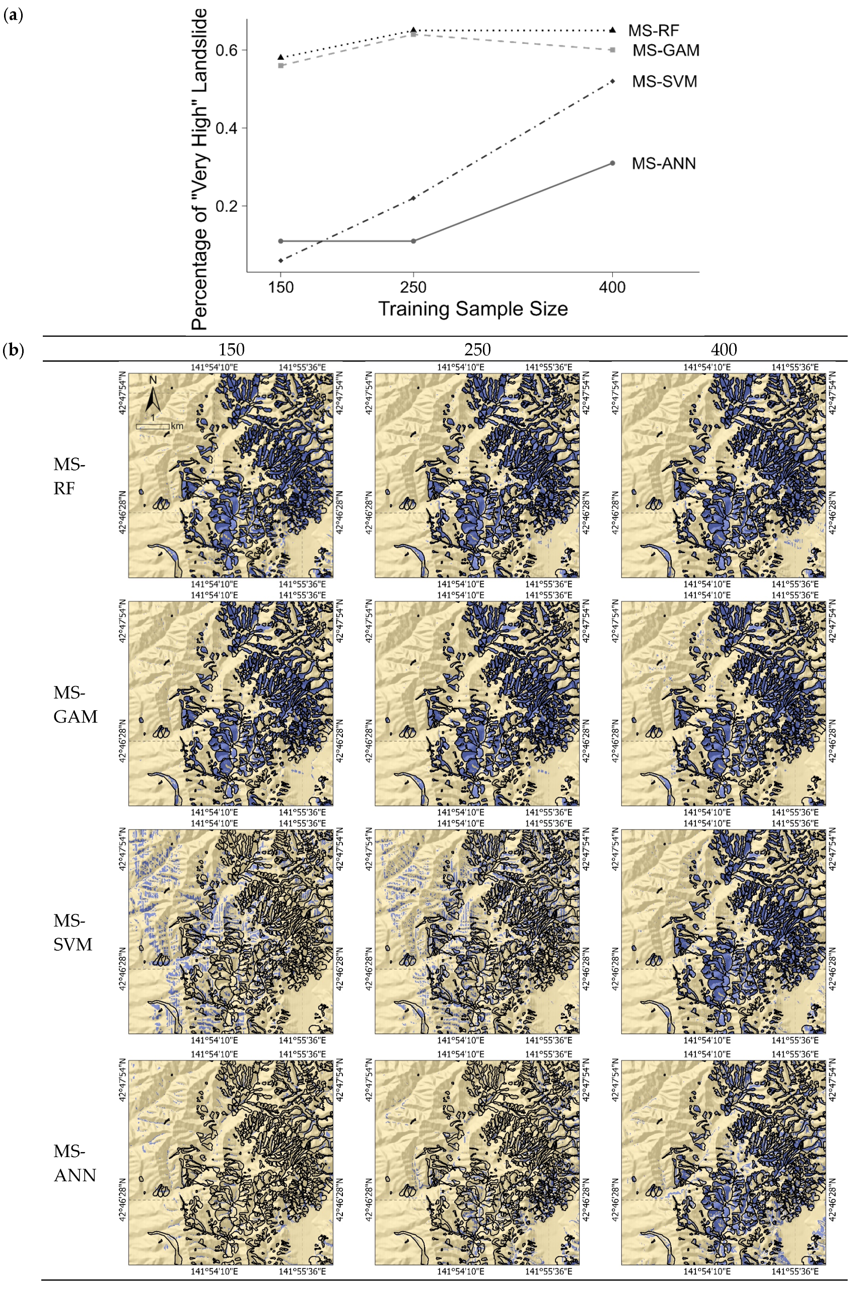
MS integrated with RF and GAM consistently demonstrated smoother and more coherent prediction surfaces in the landslide detection maps across various training instance sizes, from as few as 150 instances up to 400 (Figure 5). With a threshold based on the 96th percentile of predicted probability, these two methods produced contiguous areas with the highest likelihood of landslides (“very high”) that closely approximated the spatial extent of the landslide inventory. For the percentage of “very high” areas to the total landslide inventory, MS integrated with RF and GAM obtained much higher ratios than MS integrated with ANN and SVM, even when trained on 150 and 250 training instances. In particular, as the instance size increased from 150 to 250 and eventually to 400, MS integrated with RF continued to maintain relatively stable spatial predictions, which was consistent with the predictive accuracy (Figure 5).
In contrast, MS integrated with SVM and ANN produced more heterogeneous and fragmented prediction surfaces in the same series of maps. When only 150 to 250 total training instances were used, these models exhibited a scattered distribution of high-probability pixels that manifested as spatial artifacts across the landscape. Such artifacts not only resulted in a visually fragmented map but also in a much lower ratio of “very high” areas to the total landslide inventory, particularly at smaller training sizes. Although increasing the number of training instances to 400 mitigated these issues, the landslide detection map appearances produced by MS integrated with SVM and ANN remained less consistent compared to MS integrated with RF and GAM.

4.3. The Distribution of Landslide and Non-Landslide in the Training Set

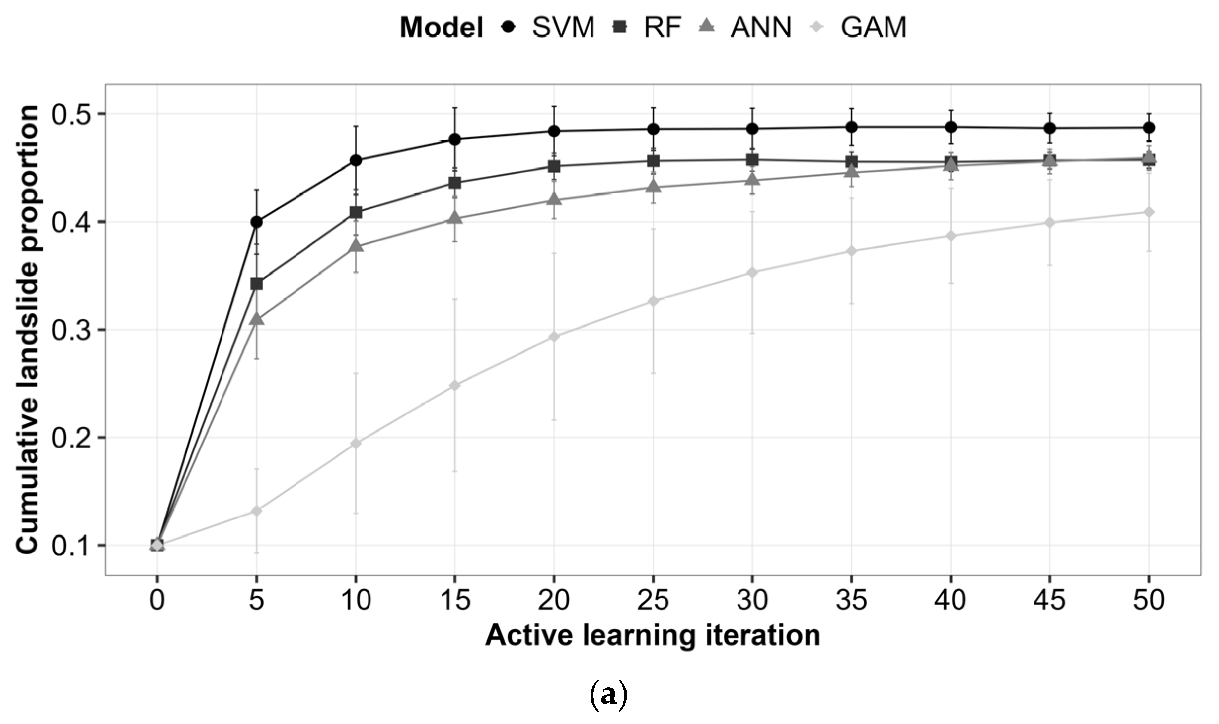
Regardless of the landslide model used, the proportion of landslide instances within the training sets obtained by all MS-based combinations showed a characteristic pattern, initially increasing and subsequently reaching a stabilization phase (Figure 6). In the initial epochs, all MS-based combinations extracted characteristics of the minority class, that is, the characteristics of landslides. For example, at epoch 5 (i.e., 225 training instances), the training set obtained by MS integrated with RF included more than 30% landslide instances. After 15 epochs (i.e., 475 training instances), the proportion of landslide instances within the training set reached approximately 45% and maintained this level throughout the subsequent epoch.
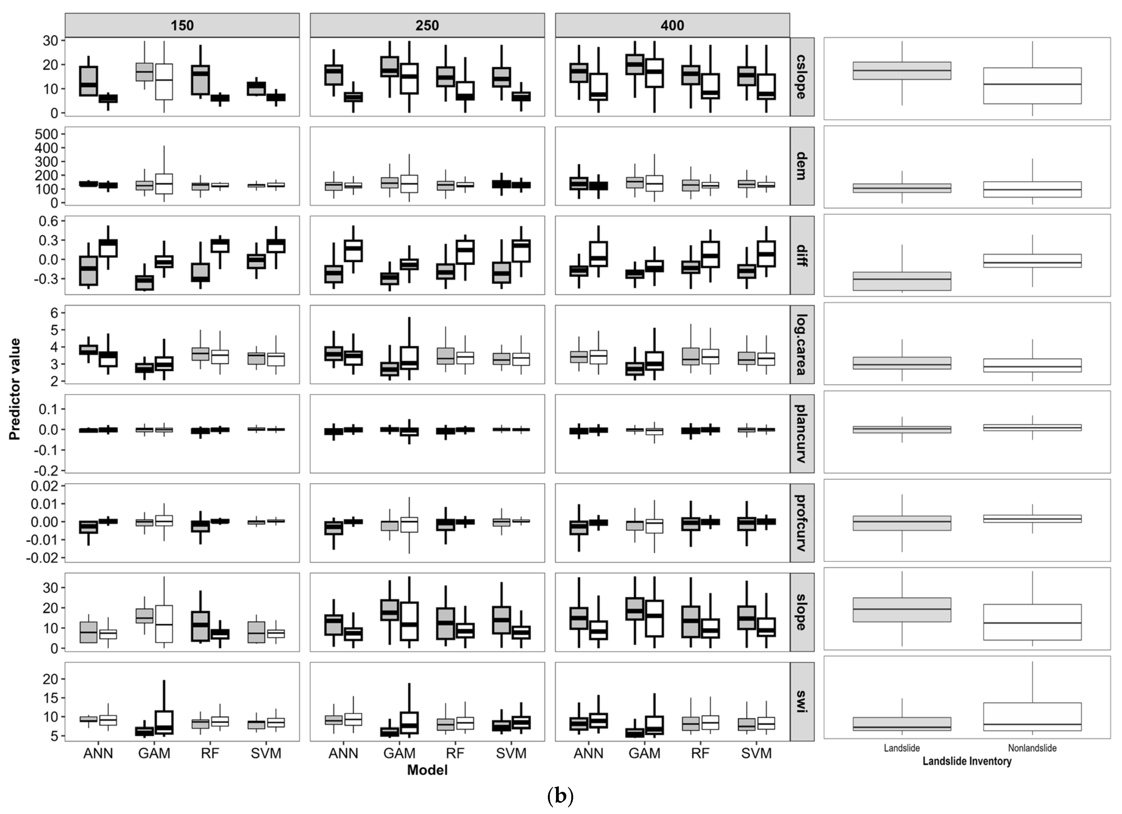
The distribution of predictor variables used for training each combination (MS integrated with SVM, RF, ANN, and GAM) displayed clear differences between landslide and non-landslide instances in the training set obtained by MS (Figure 6). For example, the landslide instances selected by all MS-based combinations had larger slope angles than the selected non-landslide instances. However, the “informative” instances identified by each combination were different. MS integrated with RF captured information for both landslide and non-landslide instances, while MS integrated with others concentrated on the information of landslide instances. For example, from 150 training instances to 250 training instances, the distribution of predictors such as the slope angle and NDVI difference in the training sets obtained by MS integrated with RF expanded for both landslide and non-landslide instances. In contrast, the distribution of predictors in the training sets obtained by MS integrated with SVM, ANN, and GAM mainly expanded for landslide instances.

4.4. A Ranking of Predictor Importance

The rank of variable importance was different for all MS-based combinations with 400 training instances, but there was some consistency in the set of highest-ranked variables (Table 3). The difference between NDVI of pre- and post- event (diff) and catchment slope angle (cslope) were always ranked in the top two based on maximum variable importance across all MS-based combinations, and the highest-ranked variable based on maximum variable importance was always the difference between NDVI of pre- and post- event. Moreover, variable importance was distributed more uniformly for the combination with lower AUROC values. For example, MS integrated with GAM, which had a lower AUROC performance than MS integrated with RF, had a larger number of variables with variable importance larger than 0.15.

5. Discussion

5.1. Impact of Model Selection on Margin Sampling

All four models obtain AUROC values above 0.90 and generate smooth, coherent landslide detection maps once the MS-selected training set reaches about 400 instances, and these performances remain stable as additional instances are added. In particular, with just 150 training instances, MS integrated with RF achieves an AUROC of 0.91, and its resulting map is smooth while capturing approximately 60% of the inventoried landslide area (Figure 4 and Figure 5). The precision-recall analysis is consistent with this interpretation. Across training sizes of 150 to 400 instances, MS integrated with RF maintains precision values of about 0.8 to 0.9 within the top 1 to 5 percent of the most susceptible areas and still achieves precision around 0.8 in the top 10 percent, while capturing roughly 40 percent of the inventoried landslide area in that limited priority zone. This comparative result aligns with the findings of [15] in a static context, yet our work extends this knowledge under an active learning regime.
Moreover, MS progressively enriches the training sets across all models. By adding MS-selected instances, the distributions of predictors for both landslide and non-landslide classes become more comprehensive. For example, leveraging MS integrated with RF, 150 training instances have already covered the full spectrum of topographic and spectral characteristics present in the inventory (Figure 6). Beyond high and stable AUROCs of all combinations, the consistency in the set of highest-ranked variables in the variable importance underscores MS’s ability to home in on the variables that matter most for landslide detection, regardless of model architecture (Table 3). In summary, MS delivers not only consistently high and stable predictive performance across diverse model architectures based on a small number of the training set, but also a laser-focus on the variables that drive landslide occurrence. Coupled with the developed Shiny GUI, this makes MS a practical framework for rapid and accurate landslide mapping in real-world settings.
The main objective of this study is to demonstrate a way to compare margin sampling-based landslide susceptibility models for spatial prediction under realistic emergency mapping constraints rather than to exhaustively explore all possible model and data configurations. Clearly, with any complex algorithm, different modeling choices or datasets may lead to different outcomes and a full evaluation of these possibilities is beyond the scope of this work.

5.2. The Importance of Training Data Quality in Landslide Detection Assessment

The training set with rich and representative information is fundamental for obtaining accurate data-driven landslide detection results. Previous studies have demonstrated that any gaps in the sampling of key characteristics of landslides and non-landslides can lead to inaccurate prediction, regardless of model sophistication [14,18]. These gaps mainly exist in information diversity and the ratio of landslides and non-landslides in the training set [42]. The information diversity in the training set impacts a model’s decision boundary. For example, in landslide hazards assessments, key variables such as slope angle, curvature metrics, and vegetation indices often show non-linear relationships with landslide occurrence [26,28]. The authors of [48] have shown that the high-quality non-landslide instances can help the model learn the features of both classes in a more balanced way. Hence, the full spectrum of features (e.g., slope angle) of each class should be considered when constructing the training set. Moreover, the ratio of landslides and non-landslides in the training set is crucial for improving the model’s sensitivity to the minority (i.e., landslide) class [14]. Yet many data-driven landslide hazard assessment studies always assumed the balance between landslide and non-landslide instances within the training set [15,18,21]. However, in real-world applications, obtaining a balanced number of landslide and non-landslide observations costs time, which can delay urgent rescue operations and reduce overall response efficiency. Our experiments show that MS automatically increases the proportion of landslides in the training set (to ~45%) without manual intervention, effectively balancing the data and ensuring key landslide characteristics are learned. In summary, MS can not only make sure of information diversity but also balance the distributions of landslide and non-landslide instances in the training set, regardless of the model used (Figure 6).
Our work not only confirms previous evidence that MS active learning can achieve rapid and precise landslide hazard assessment [12,13], but also fills a critical gap by comparing the performances of MS integrated with different modeling approaches (i.e., RF, SVM, GAM, and ANN). In addition, we have developed an RShiny GUI that integrates MS with RF, SVM, GAM, and ANN, providing an interactive environment for uploading data, configuring models, querying uncertain instances, and updating labels in real time. In the future, this GUI can be adapted to diverse geographic regions and extended to other environmental hazards (e.g., flood and wildfire detection) to construct high-quality training datasets. Further efforts should focus on coupling the interface with cloud-based geospatial platforms (e.g., Google Earth Engine) for interactive instance visualization and annotation at scale.

5.3. Limitations and Outlook

A key limitation of this study is that the integration of active learning and four machine learning methods were evaluated on a single landslide event in one region, namely the Iburi earthquake-triggered inventory in Hokkaido, Japan. Although this dataset is large, internally consistent, and openly available, the restriction to one geographic and triggering context means that the spatial generalizability of our findings remains constrained. Conditioning factors that control landslide occurrence, such as lithology, soil properties, vegetation structure, land use, relief, and climatic regime, can differ substantially in other mountain belts and especially in tropical or subtropical environments. Likewise, the Iburi event represents co-seismic landslides, whereas rainfall-induced, snowmelt-related, or anthropogenic failures may respond differently to both predictors and active learning strategies.
For future research, this comparative study will extend to additional inventories from different climatic zones and geomorphic settings and to perform cross-area evaluations in which models are trained in one region and tested in another. Such experiments would provide a more direct assessment of transferability and would reveal whether the same active learning settings and model choices remain efficient under different landslide regimes. In addition, future applications could couple this framework with explicit representations of triggering processes by including seismic shaking parameters such as peak ground acceleration or intensity and rainfall metrics for storm driven events as additional predictors or conditioning variables. This would allow the active learning system to reflect the spatial distribution of different triggers and to test whether the sampling strategy remains efficient when multiple hazards interact.

6. Conclusions

To evaluate the effectiveness of the MS active learning for rapid and accurate landslide mapping, we conducted a comparison of MS integrated with four commonly used landslide modeling techniques (i.e., RF, SVM, GAM, and ANN). This comparable study demonstrated that MS was highly effective for rapid and accurate landslide mapping regardless of the modeling algorithm used, as all models (i.e., RF, SVM, GAM, and ANN) achieved >0.90 accuracy with small training sets. Among them, MS integrated with RF reached an AUROC of 0.91 with only 150 training instances, followed closely by MS integrated with SVM. Furthermore, we developed a Shiny-based GUI, which ensures full reproducibility and technology transfer, lowering the barrier for researchers and practitioners to implement rapid landslide mapping in their own regions. In summary, this work not only advances our theoretical understanding of active learning in landslide detection but also provides practical tools to improve rapid hazard assessment workflows, potentially saving time in response scenarios. However, the study is limited to a single region and trigger, and results may differ in other settings. Future work should test the framework in diverse geographic and hazard contexts (e.g., rain-induced landslides) to generalize findings as well as extend GUI capabilities (e.g., integrating cloud-based geospatial platforms). We also foresee adapting the framework for multi-hazard scenarios, such as incorporating real-time seismic measurements to map earthquake-triggered landslides or coupling it with rainfall thresholds for storm-induced landslides, thereby broadening its applicability.

Author Contributions

Conceptualization, Methodology, Software, Validation, Formal Analysis, Visualization, Writing—Original Draft: J.M. and Z.W. (Zhihao Wang); Funding Acquisition, Writing—Review and Editing: C.L.; Writing—Review and Editing: J.M., D.Y., and Z.W. (Zhichao Wang). All authors have read and agreed to the published version of the manuscript.

Funding

This research was funded by Natural Science Basic Research Program of Shaanxi (Program No. 2025JC-YBQN-395) and China Postdoctoral Science Foundation (No. 2023M742729).

Data Availability Statement

The data presented in this study are available in Zenodo at https://zenodo.org/record/2577300 (CC BY 4.0) (accessed on 26 November 2025), reference [16]. These data were derived from the following resources available in the public domain: (i) Landslide inventories: Zenodo record https://zenodo.org/record/2577300 (CC BY 4.0) (accessed on 26 November 2025); (ii) Digital Elevation Model (DEM): Geospatial Information Authority of Japan (GSI), downloadable at https://fgd.gsi.go.jp/download/menu.php (accessed on 26 November 2025). Code Availability Statement: The graphical user interface that integrates margin sampling active learning with random forest, support vector machine, generalized additive model, and artificial neural network are available at Github (https://github.com/W-Zhihao/MS_SampleSelection.git) (accessed on 26 November 2025).

Conflicts of Interest

The authors declare no conflicts of interest. Author Jing Miao is employed by the company Space Star Technology Co., Ltd. The remaining authors declare that the research was conducted in the absence of any commercial or financial relationships that could be construed as a potential conflict of interest. Space Star Technology Co., Ltd had no role in the design of the study; in the collection, analyses, or interpretation of data; in the writing of the manuscript, or in the decision to publish the results.

References

  1. Froude, M.J.; Petley, D.N. Global Fatal Landslide Occurrence from 2004 to 2016. Nat. Hazards Earth Syst. Sci. 2018, 18, 2161–2181. [Google Scholar] [CrossRef]
  2. Merghadi, A.; Yunus, A.P.; Dou, J.; Whiteley, J.; ThaiPham, B.; Bui, D.T.; Avtar, R.; Abderrahmane, B. Machine Learning Methods for Landslide Susceptibility Studies: A Comparative Overview of Algorithm Performance. Earth-Sci. Rev. 2020, 207, 103225. [Google Scholar] [CrossRef]
  3. Mohan, A.; Singh, A.K.; Kumar, B.; Dwivedi, R. Review on Remote Sensing Methods for Landslide Detection Using Machine and Deep Learning. Trans. Emerg. Telecommun. Technol. 2021, 32, e3998. [Google Scholar] [CrossRef]
  4. Fu, L.; Zhang, Q.; Wang, T.; Li, W.; Xu, Q.; Ge, D. Detecting Slow-Moving Landslides Using InSAR Phase-Gradient Stacking and Deep-Learning Network. Front. Environ. Sci. 2022, 10, 963322. [Google Scholar] [CrossRef]
  5. Casagli, N.; Frodella, W.; Morelli, S.; Tofani, V.; Ciampalini, A.; Intrieri, E.; Raspini, F.; Rossi, G.; Tanteri, L.; Lu, P. Spaceborne, UAV and Ground-Based Remote Sensing Techniques for Landslide Mapping, Monitoring and Early Warning. Geoenviron. Disasters 2017, 4, 9. [Google Scholar] [CrossRef]
  6. Cheng, Y.; Pang, H.; Li, Y.; Fan, L.; Wei, S.; Yuan, Z.; Fang, Y. Applications and Advancements of Spaceborne InSAR in Landslide Monitoring and Susceptibility Mapping: A Systematic Review. Remote Sens. 2025, 17, 999. [Google Scholar] [CrossRef]
  7. Tsironi, V.; Ganas, A.; Karamitros, I.; Efstathiou, E.; Koukouvelas, I.; Sokos, E. Kinematics of Active Landslides in Achaia (Peloponnese, Greece) through InSAR Time Series Analysis and Relation to Rainfall Patterns. Remote Sens. 2022, 14, 844. [Google Scholar] [CrossRef]
  8. Mondini, A.C.; Guzzetti, F.; Chang, K.-T.; Monserrat, O.; Martha, T.R.; Manconi, A. Landslide Failures Detection and Mapping Using Synthetic Aperture Radar: Past, Present and Future. Earth-Sci. Rev. 2021, 216, 103574. [Google Scholar] [CrossRef]
  9. Ado, M.; Amitab, K.; Maji, A.K.; Jasińska, E.; Gono, R.; Leonowicz, Z.; Jasiński, M. Landslide Susceptibility Mapping Using Machine Learning: A Literature Survey. Remote Sens. 2022, 14, 3029. [Google Scholar] [CrossRef]
  10. Settles, B. Active Learning; Synthesis Lectures on Artificial Intelligence and Machine Learning; Springer International Publishing: Cham, Switzerland, 2012; ISBN 978-3-031-00432-2. [Google Scholar]
  11. Lin, J.; Zhao, L.; Li, S.; Ward, R.; Wang, Z.J. Active-Learning-Incorporated Deep Transfer Learning for Hyperspectral Image Classification. IEEE J. Sel. Top. Appl. Earth Obs. Remote Sens. 2018, 11, 4048–4062. [Google Scholar] [CrossRef]
  12. Wang, Z.; Brenning, A. Active-Learning Approaches for Landslide Mapping Using Support Vector Machines. Remote Sens. 2021, 13, 2588. [Google Scholar] [CrossRef]
  13. Wang, Z.; Brenning, A. Unsupervised Active–Transfer Learning for Automated Landslide Mapping. Comput. Geosci. 2023, 181, 105457. [Google Scholar] [CrossRef]
  14. Liu, S.; Wang, L.; Zhang, W.; He, Y.; Pijush, S. A Comprehensive Review of Machine Learning-Based Methods in Landslide Susceptibility Mapping. Geol. J. 2023, 58, 2283–2301. [Google Scholar] [CrossRef]
  15. Goetz, J.N.; Brenning, A.; Petschko, H.; Leopold, P. Evaluating Machine Learning and Statistical Prediction Techniques for Landslide Susceptibility Modeling. Comput. Geosci. 2015, 81, 1–11. [Google Scholar] [CrossRef]
  16. Huang, Y.; Zhao, L. Review on Landslide Susceptibility Mapping Using Support Vector Machines. CATENA 2018, 165, 520–529. [Google Scholar] [CrossRef]
  17. Tien Bui, D.; Tuan, T.A.; Klempe, H.; Pradhan, B.; Revhaug, I. Spatial Prediction Models for Shallow Landslide Hazards: A Comparative Assessment of the Efficacy of Support Vector Machines, Artificial Neural Networks, Kernel Logistic Regression, and Logistic Model Tree. Landslides 2016, 13, 361–378. [Google Scholar] [CrossRef]
  18. Bordoni, M.; Galanti, Y.; Bartelletti, C.; Persichillo, M.G.; Barsanti, M.; Giannecchini, R.; Avanzi, G.D.; Cevasco, A.; Brandolini, P.; Galve, J.P.; et al. The Influence of the Inventory on the Determination of the Rainfall-Induced Shallow Landslides Susceptibility Using Generalized Additive Models. CATENA 2020, 193, 104630. [Google Scholar] [CrossRef]
  19. Zhang, S.; Li, R.; Wang, F.; Iio, A. Characteristics of Landslides Triggered by the 2018 Hokkaido Eastern Iburi Earthquake, Northern Japan. Landslides 2019, 16, 1691–1708. [Google Scholar] [CrossRef]
  20. Plank, S.; Twele, A.; Martinis, S. Landslide Mapping in Vegetated Areas Using Change Detection Based on Optical and Polarimetric SAR Data. Remote Sens. 2016, 8, 307. [Google Scholar] [CrossRef]
  21. Asadi, M.; Goli Mokhtari, L.; Shirzadi, A.; Shahabi, H.; Bahrami, S. A Comparison Study on the Quantitative Statistical Methods for Spatial Prediction of Shallow Landslides (Case Study: Yozidar-Degaga Route in Kurdistan Province, Iran). Environ. Earth Sci. 2022, 81, 51. [Google Scholar] [CrossRef]
  22. Zhang, W.; Liu, S.; Wang, L.; Samui, P.; Chwała, M.; He, Y. Landslide Susceptibility Research Combining Qualitative Analysis and Quantitative Evaluation: A Case Study of Yunyang County in Chongqing, China. Forests 2022, 13, 1055. [Google Scholar] [CrossRef]
  23. Thang, N.V.; Wakai, A.; Sato, G.; Viet, T.T.; Kitamura, N. Simple Method for Shallow Landslide Prediction Based on Wide-Area Terrain Analysis Incorporated with Surface and Subsurface Flows. Nat. Hazards Rev. 2022, 23, 04022028. [Google Scholar] [CrossRef]
  24. Arango, M.I.; Aristizábal, E.; Gómez, F. Morphometrical Analysis of Torrential Flows-Prone Catchments in Tropical and Mountainous Terrain of the Colombian Andes by Machine Learning Techniques. Nat. Hazards 2021, 105, 983–1012. [Google Scholar] [CrossRef]
  25. Małka, A. Landslide Susceptibility Mapping of Gdynia Using Geographic Information System-Based Statistical Models. Nat. Hazards 2021, 107, 639–674. [Google Scholar] [CrossRef]
  26. Muenchow, J.; Brenning, A.; Richter, M. Geomorphic Process Rates of Landslides along a Humidity Gradient in the Tropical Andes. Geomorphology 2012, 139–140, 271–284. [Google Scholar] [CrossRef]
  27. Planet Team. Planet Application Program Interface. In Space for Life on Earth; Planet Team: San Francisco, CA, USA, 2017; Volume 2017, p. 2. Available online: https://api.planet.com (accessed on 5 November 2025).
  28. Fiorucci, F.; Ardizzone, F.; Mondini, A.C.; Viero, A.; Guzzetti, F. Visual Interpretation of Stereoscopic NDVI Satellite Images to Map Rainfall-Induced Landslides. Landslides 2019, 16, 165–174. [Google Scholar] [CrossRef]
  29. Hastie, T.J. Generalized Additive Models. In Statistical Models in S.; Routledge: New York, NY, USA, 1992; ISBN 978-0-203-73853-5. [Google Scholar]
  30. Yaghoubzadeh-Bavandpour, A.; Rajabi, M.; Nozari, H.; Ahmad, S. Support Vector Machine Applications in Water and Environmental Sciences. In Computational Intelligence for Water and Environmental Sciences; Bozorg-Haddad, O., Zolghadr-Asli, B., Eds.; Springer Nature: Singapore, 2022; pp. 291–310. ISBN 978-981-19-2519-1. [Google Scholar]
  31. Tyralis, H.; Papacharalampous, G.; Langousis, A. A Brief Review of Random Forests for Water Scientists and Practitioners and Their Recent History in Water Resources. Water 2019, 11, 910. [Google Scholar] [CrossRef]
  32. Hsieh, W.W. Machine Learning Methods in the Environmental Sciences: Neural Networks and Kernels; Cambridge University Press: Cambridge, UK, 2009; ISBN 978-0-521-79192-2. [Google Scholar]
  33. Wood, S.N. Generalized Additive Models: An Introduction with R, Second Edition; Chapman and Hall/CRC: New York, NY, USA, 2017; ISBN 978-1-315-37027-9. [Google Scholar]
  34. Wood, S. Mgcv: Mixed GAM Computation Vehicle with Automatic Smoothness Estimation, R Package Version 1.8–12; R Core Team: Vienna, Austria, 2023.
  35. Van Engelen, J.E.; Hoos, H.H. A Survey on Semi-Supervised Learning. Mach. Learn. 2020, 109, 373–440. [Google Scholar] [CrossRef]
  36. Marjanović, M.; Kovačević, M.; Bajat, B.; Voženílek, V. Landslide Susceptibility Assessment Using SVM Machine Learning Algorithm. Eng. Geol. 2011, 123, 225–234. [Google Scholar] [CrossRef]
  37. Hong, H.; Pradhan, B.; Jebur, M.N.; Bui, D.T.; Xu, C.; Akgun, A. Spatial Prediction of Landslide Hazard at the Luxi Area (China) Using Support Vector Machines. Environ. Earth Sci. 2015, 75, 40. [Google Scholar] [CrossRef]
  38. Kuhn, M.; Wing, J.; Weston, S.; Williams, A.; Keefer, C.; Engelhardt, A.; Cooper, T.; Mayer, Z.; Kenkel, B.; Benesty, M. Caret: Classification and Regression Training; R Core Team: Vienna, Austria, 2024. [Google Scholar]
  39. Breiman, L. Random Forests. Mach. Learn. 2001, 45, 5–32. [Google Scholar] [CrossRef]
  40. Zhang, Y.; Wu, W.; Qin, Y.; Lin, Z.; Zhang, G.; Chen, R.; Song, Y.; Lang, T.; Zhou, X.; Huangfu, W.; et al. Mapping Landslide Hazard Risk Using Random Forest Algorithm in Guixi, Jiangxi, China. ISPRS Int. J. Geo-Inf. 2020, 9, 695. [Google Scholar] [CrossRef]
  41. Huang, Y.; Wänstedt, S. The Introduction of Neural Network System and Its Applications in Rock Engineering. Eng. Geol. 1998, 49, 253–260. [Google Scholar] [CrossRef]
  42. Pradhan, B.; Youssef, A.; Varathrajoo, R. Approaches for Delineating Landslide Hazard Areas Using Different Training Sites in an Advanced Artificial Neural Network Model. Geo-Spat. Inf. Sci. 2010, 13, 93–102. [Google Scholar] [CrossRef]
  43. Pardeshi, S.D.; Autade, S.E.; Pardeshi, S.S. Landslide Hazard Assessment: Recent Trends and Techniques. SpringerPlus 2013, 2, 523. [Google Scholar] [CrossRef] [PubMed]
  44. Beguería, S. Validation and Evaluation of Predictive Models in Hazard Assessment and Risk Management. Nat. Hazards 2006, 37, 315–329. [Google Scholar] [CrossRef]
  45. Frattini, P.; Crosta, G.; Carrara, A. Techniques for Evaluating the Performance of Landslide Susceptibility Models. Eng. Geol. 2010, 111, 62–72. [Google Scholar] [CrossRef]
  46. Strobl, C.; Boulesteix, A.-L.; Zeileis, A.; Hothorn, T. Bias in Random Forest Variable Importance Measures: Illustrations, Sources and a Solution. BMC Bioinform. 2007, 8, 25. [Google Scholar] [CrossRef]
  47. Brenning, A.; Long, S.; Fieguth, P. Detecting Rock Glacier Flow Structures Using Gabor Filters and IKONOS Imagery. Remote Sens. Environ. 2012, 125, 227–237. [Google Scholar] [CrossRef]
  48. Gu, T.; Duan, P.; Wang, M.; Li, J.; Zhang, Y. Effects of Non-Landslide Sampling Strategies on Machine Learning Models in Landslide Susceptibility Mapping. Sci. Rep. 2024, 14, 7201. [Google Scholar] [CrossRef]
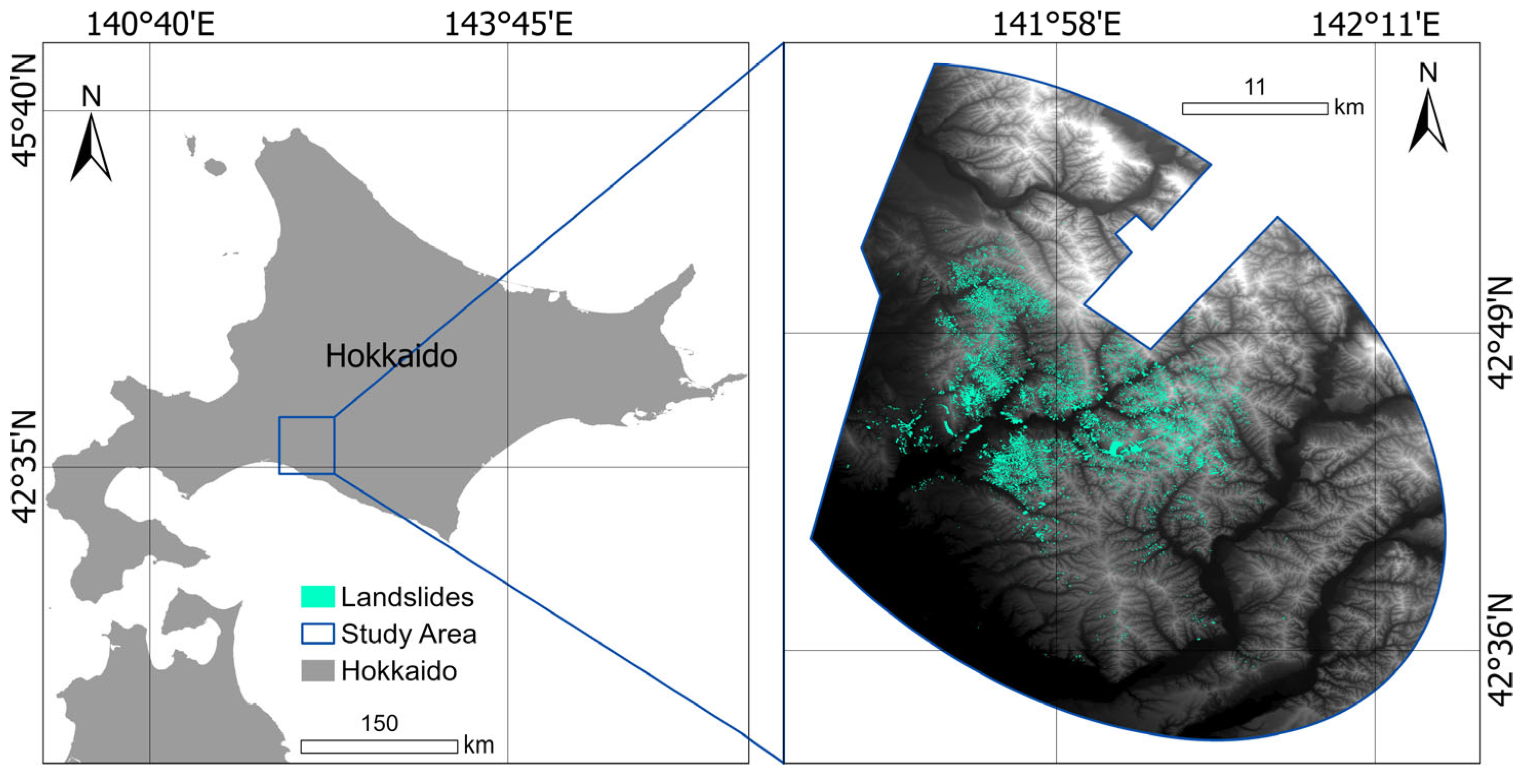
Figure 1. The study area of Hokkaido (the blue rectangles) and landslide inventories.
Geomatics 05 00074 g001
Figure 2. The workflow of the margin sampling active learning framework integrating with GAM, RF, SVM, and ANN.
Geomatics 05 00074 g002
Figure 3. Graphical user interface integrating MS with four machine learning algorithms (SVM, RF, ANN, and GAM) for the iterative selection of “informative” training instances.
Geomatics 05 00074 g003
Figure 4. Comparison of four combinations (MS with RF, SVM, ANN, and GAM). (a) Mean AUROC values and (b) Standard deviation of AUROC values over 100 repetitions under varied training instance sizes.
Geomatics 05 00074 g004
Figure 5. Comparison of performances of different combinations (MS with RF, GAM, SVM, and ANN) in landslide detection maps based on 150, 250, and 400 training instances in the 7th repetition: (a) the percentage of areas with the highest likelihood of landslides (“very high”, purple) out of the total landslide area derived from the landslide inventory obtained by each combination based on 150, 250, and 400 training instances; (b) an example of classified landslide detection maps for each combination. The detected “very high” landslide area is based on predicted probabilities above the 96th percentile.
Geomatics 05 00074 g005
Figure 6. (a) The distribution of landslide and non-landslide in the training set: the average proportion of landslide instances in the training set across 50 epochs of 100 repetitions obtained by all combinations (MS integrated with SVM, RF, ANN, and GAM); (b) The distribution of eight predictor variables, i.e., slope angle (°, slope), plan curvature (radians per 100 m, plancurv), profile curvature (radians per 100 m, profcurv), log transformed upslope contributing area (log10 m2, log.carea), elevation (m, dem), SWI, catchment slope angle (cslope), and NDVI difference (diff), under both landslide (gray boxes) and non-landslide (white boxes) conditions in 150, 250, and 400 training instance obtained by all combinations (MS integrated with SVM, RF, ANN, and GAM) in the 7th repetition and the whole landslide inventory. Bolded boxes indicate that the variable shows the significant difference in landslides and non-landslides under the current model and current training set with the p-value 0.05 threshold obtained by the Wilcoxon test.
Geomatics 05 00074 g006aGeomatics 05 00074 g006b
Table 1. The information about Iburi landslide inventory, including median and interquartile range (IQR) values of predictor variables for landslide and non-landslide instances in the study area and type and characteristic information of landslides.
Predictor VariableLandslides Median (IQR)Non-Landslides Median (IQR)Data Source
slope angle (°, slope)18.51 (11.42)9.88 (17.54)DEM with a 10 m × 10 m resolution
plan curvature (radians per 100 m, plancurv)−0.00007 (0.01242)0.00105 (0.02024)
profile curvature (radians per 100 m, profcurv)−0.00029 (0.00448)0.0000 (0.00295)
upslope contributing area (log10 m2, log.carea)2.72 (0.65)2.91 (0.67)
elevation (m, dem)138.7 (73.99)117.75 (139.1)
SWI5.72 (2.05)7.38 (6.76)
catchment slope angle (cslope)19.46 (8.04)10.95 (14.81)
NDVI difference (diff)−0.29 (0.28)−0.03 (0.21)PlanetScope optical images with a 3 m × 3 m resolution
landslide typeco-seismic landslides
landslide processshallow debris slides
triggering mechanismearthquake
geological unitssedimentary and volcanic rocks
Table 2. Mean AUROC and precision–recall statistics at different areal fractions (percentile) for MS combined with four landslide modeling algorithms in 150, 250, and 400 training sizes.
Training SizeModelMean AUROCTop 1%Top 2%Top 4%Top 5%Top 10%
PrecisionRecallPrecisionRecallPrecisionRecallPrecision RecallPrecisionRecall
150ANN0.790.750.040.740.080.700.150.680.180.600.31
GAM0.720.760.040.710.070.680.480.700.180.660.35
RF0.860.910.050.900.090.880.190.870.230.800.42
SVM0.670.550.030.520.050.490.100.480.120.420.22
250ANN0.870.810.040.800.080.780.160.770.200.730.38
GAM0.760.830.040.800.080.770.370.780.200.740.39
RF0.890.860.040.860.090.850.180.840.220.810.42
SVM0.830.900.050.890.090.860.180.850.220.760.40
400ANN0.890.810.040.830.090.830.180.820.210.770.40
GAM0.810.880.050.870.090.850.270.850.220.790.41
RF0.900.860.040.850.090.840.180.830.220.800.42
SVM0.900.850.040.840.090.830.170.830.220.790.41
Table 3. Variable importance based on median AUROC values from cross-validation based on 400 training points. The values are standardized relative to the most important predictor variable for each combination.
VariableRankMax Variable ImportanceMS-GAMMS-ANNMS-SVMMS-RF
diff111111
cslope20.780.780.480.320.25
log.carea30.550.5500.10
SWI40.520.520.110.080.1
slope50.350.350.0700.11
plancurv60.130.130.040.130.05
dem70.120.020.120.040.06
profcurv80.0900.030.030.09
Disclaimer/Publisher’s Note: The statements, opinions and data contained in all publications are solely those of the individual author(s) and contributor(s) and not of MDPI and/or the editor(s). MDPI and/or the editor(s) disclaim responsibility for any injury to people or property resulting from any ideas, methods, instructions or products referred to in the content.