Abstract
Horizontal dilution of precision (HDOP) is a widely used quality indicator of Global Navigation Satellite System (GNSS) positioning, considering only satellite geometry. In this study, HDOP was simulated using GNSS almanacs and high-resolution digital surface models (DSMs) along three European road sections: Oslo— Svinesund Bridge (Norway); Hamburg city center (Germany); and Rotterdam—Dutch–German border (Netherlands). This study was accomplished as part of the MODI project, which is a cross-border initiative to accelerate Cooperative, Connected, and Automated Mobility (CCAM). Our analysis revealed excellent or good overall GNSS performance in the study areas, particularly on highway sections with 99–100% of study points having a median HDOP that is categorized as excellent (HDOP < 2) or good (HDOP < 5). However, the road section in Hamburg’s city center presents challenges. When GPS is used alone, 8% of the study points experience weak or poor HDOP, and there are study points where the system is available (HDOP < 5) less than 50% of the time. Combining GNSS constellations significantly improved system availability, reaching 95% for 99% of the study points in Hamburg. To validate our simulations, we compared results with GNSS observations from a survey vehicle in Hamburg. Initial low correlation was attributed to the reception of signals from non-line-of-sight satellites. By excluding satellites with low signal-to-noise ratios, the correlation increased significantly, and reasonable agreement was obtained. We also examined the impact of using a 10 m DSM instead of a 1 m DSM in Hamburg. While the coarser spatial resolution offers computational benefits, it may miss critical details for accurate assessment of satellite visibility.
1. Introduction
The MODI project (the project name MODI is based on the Norwegian word for being brave, modig) (https://modiproject.eu, accessed on 1 June 2025), funded under the European Union’s research and innovation program Horizon Europe, is a cross-border initiative to accelerate the introduction of Cooperative, Connected, and Automated Mobility (CCAM) solutions and to improve European logistic chains [1]. Work package four of the project focuses on coordinated CCAM interface and physical–digital infrastructure. A key objective is to demonstrate what is needed to have automated freight transport in the MODI corridor that passes through the five European countries of Norway, Sweden, Denmark, Germany, and the Netherlands (see Figure 1). A current issue in this context is what Global Navigation Satellite System (GNSS) performance can be expected along the road corridors. For automotive applications, accurate GNSS positioning is especially relevant with the introduction of CCAM and advanced driver assistant systems, where GNSS is proposed to support precise vehicle positioning, control of the vehicle’s movement, navigation, emergency services, road tolling, pay-as-you-drive insurance, fleet management, cooperation between vehicles, and more (see, e.g., [2]).
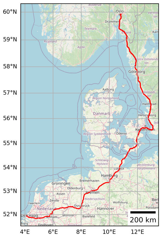
Figure 1.
The MODI corridor is in total ca. 1460 km long and passes through five European countries (Norway, Sweden, Denmark, Germany, and the Netherlands) from Oslo in Norway to Rotterdam in the Netherlands. Basemap from OpenStreetMap [3].
GNSS positioning accuracy along road corridors depends on the availability and distribution of satellites in the sky [4]. Dilution of precision (DOP) is a widely used quality indicator for GNSS positioning [5] and quantifies the impact of satellite geometry on positioning accuracy. It varies with location and time, and it reflects the geometrical distribution of about 130 GNSS satellites that presently exist in orbit (GPS: 30, GLONASS: 24, GALILEO: 27, and BeiDou: 51 as of June 2025). The DOP takes into account only the geometry of the GNSS constellations, and signal disturbances and accuracy degradation due to errors in satellite ephemerides, multipath and atmospheric propagation delays are not considered. This implies that many well-distributed satellites result in a low DOP, indicating potentially high positioning accuracy. In contrast, few satellites, only satellites close to zenith, or satellites clustered in only one direction result in a higher DOP and potentially low positioning accuracy or even conditions that make positioning, navigation, and timing based on GNSS impossible. Simulated DOP has, therefore, the potential to predict expected GNSS performance and can be useful to identify potentially challenging areas.
For simulating accurate and relevant DOP values, effects of terrain and other obstacles hampering satellite visibility must be taken into account [6]. Considering automated mobility, this is particularly important for road sections surrounded by, e.g., tall buildings, bridges, trees, and steep land formations like valleys and mountains. It is therefore unfortunate that freely available GNSS planning tools like Trimble GNSS planning and Navmatix GNSS planning (available at www.gnssplanning.com and www.gnssmissionplanning.com, accessed on 1 June 2025) do not allow modelling of terrain and other obstacles. Furthermore, it is also common that GNSS planning tools examine only a single study point at a time. This makes them unsuitable for analyzing complex road sections where DOP must be calculated at many locations.
There are still more advanced tools developed for collecting and analyzing information about the GNSS signal-propagation environment. Such tools are often called GNSS feature maps and aim at representing signal reflections, deflection, and multipath environments. Simulated DOP may play an important role for GNSS feature maps by providing a geometrical quality indicator that complements the environmental information. GNSS feature maps can be used to aid trajectory planning by identifying GNSS-friendly routes and to exclude observations from non-line-of-sight (NLOS) satellites or, alternatively, to correct NLOS or multipath errors in order to enhance the positioning accuracy.
GNSS feature maps have been implemented in several previous studies. Ruwisch and Schön [7] demonstrate how a GNSS feature map can be used to compute weights for GNSS observations in an RTK positioning algorithm. The methodology improved their root mean square error (RMSE) of horizontal positioning by 90.5%, and the maximum horizontal position error was reduced from 2.45 m to 0.52 m. In [8], the Receiver Autonomous Integrity Monitoring method was applied to exclude GNSS measurements inconsistent with pseudoranges simulated by combining 3D building models and ray-tracing techniques. This led to a reduction in the number of positioning solutions with large errors by 8.4% and 36.2% in the middle and deep urban canyon environments, respectively. Also, Wang et al. [9] benefited from 3D city models. They combined these models with GNSS ephemerides to predict satellite visibility in urban environments. The simulations were verified both at test points and along vehicle routes. They concluded that simulations are useful to predict the best route through a city at a given time or the best time to perform GNSS positioning at a given location. The authors suggested using similar techniques to assess GNSS performance in mountainous areas but with digital elevation models replacing the city model. A third example of using building models can be found in Kleijer et al. [10], simulating GNSS performance at the Schiphol Airport, the Netherlands. The simulations indicate that the GNSS availability is seriously degraded by buildings that block the line of sight to the satellites from more than one side. While 95% availability can be reached by GPS alone under mild conditions (20 m wide streets surrounded by 8 m high buildings), 95% availability cannot be reached everywhere and at any time, even when three GNSS constellations are combined. A detailed assessment of satellite visibility and simulations of DOP was successfully accomplished by Gandolfi and La Via [6], who developed open-source software for GNSS planning and simulations using a digital elevation model to create realistic maps of obstacles. The software can be run in “area mode”, allowing DOP to be calculated in multiple points within a study area.
To assess GNSS performance along the MODI project corridor, we need to evaluate DOP and satellite visibility at study points spread over long distances and located in varying environments. To solve this challenge, we developed in-house software tailored for computing DOP at study points located at polylines that in this study represent road sections. Furthermore, the software uses gridded high-resolution digital surface models (DSMs) to evaluate the effects of the surrounding topography and other obstacles. In general, such models are more widely available compared to 3D building models or city models but lack detailed representations of, e.g., building facades. We focused on three study areas centered around the southbound highway from Oslo to Svinesund Bridge (122 km) at the Norwegian–Swedish border, Hamburg City (42 km), Germany, and the northbound highway from Rotterdam to the Dutch–German border (268 km). Along these road corridors, we simulated DOP at thousands of study points and for 96 epochs evenly spaced throughout the day of 3 April 2024. The main objective of this study is to demonstrate how simulations of DOP can be used to identify areas where GNSS positioning accuracy potentially is low. We also investigate the benefit of combining several GNSS constellations in challenging areas and check if improved positioning accuracy can be obtained by visiting challenging areas at specific times. The benefits of high-spatial-resolution DSMs come at the cost of simulations with a high computational burden. We therefore also address to what degree comparable results may be obtained by using a DSM with, e.g., 10 m resolution instead of 1 m. Finally, we assess the simulated DOP by comparing it with DOP derived from GNSS observations collected by a survey vehicle in Hamburg.
One important restriction of the present study is that it focuses on Single Point Positioning (SPP), i.e., the position is obtained with a single GNSS receiver and no additional information from reference stations or a GNSS correction service. With SPP, the positioning accuracy is typically better than 13 m (two times the distance of RMS) [11], which is sufficiently accurate for navigation, tracking vehicles, and determining which road a vehicle is traveling along. However, SPP lacks the accuracy required for, e.g., precise in-lane positioning and assisted driving maneuvers like lane changing (see [2,12]). Such applications require the accuracy of real-time kinematic differential GNSS, which offers centimeter precision [13]. Since all GNSS positioning techniques rely on visible GNSS satellites, it is still appropriate to focus on SPP for identifying challenging areas along a road corridor with a view to GNSS visibility. We do not consider sensor fusion in this study, either. Sensor fusion combines absolute positioning from GNSS with measurements from vehicle sensors like accelerometers, wheel speed sensors, steering wheel angle sensors, and odometers for more robust positioning. This is despite the acknowledged importance of sensor fusion for reliable positioning and navigation, especially in areas with limited GNSS visibility or signal outages (see, e.g., [14,15]).
2. Materials and Methods
Prototype software was written in Python (version 3.9) to simulate DOP at study points along defined road corridors and selected epochs, considering effects of terrain, buildings, and other obstacles that potentially block signals from GNSS satellites. It allows simulations to be performed for cases depending on one or several GNSS constellations. The simulations depend on accurate high-resolution DSMs and satellite positions calculated from GNSS almanacs.
2.1. Digital Surface Models
Digital surface models (DSMs) mimic the elevation of the surface of the Earth, including vegetation and artificial objects like, e.g., buildings, bridges, wind turbines, and powerlines. This is in contrast to digital terrain models (DTMs) that include only the bare topography of the Earth and 3D building models that represent the surfaces of buildings and normally not the topography of the terrain. To accurately calculate DOP, DSMs play a vital role in assessing the visibility of satellites. Only satellites with an elevation angle greater than the elevation angle of the DSM in the direction of question should be considered as visible and included in the calculation of the DOP.
DSMs are also used for interpolating heights of the study points along road corridors. These heights are necessary for calculating the elevation angle to both satellites and the surrounding terrain points. To assign correct heights, quite accurate horizontal positions of the road are necessary, and we used road polylines digitized from large-scale maps provided by OpenStreetMaps [3]. Accurate representations of roads are especially important for segments that are raised or lowered with respect to their immediate surroundings, e.g., roads on bridges. A slight error in the road representation may in such situations imply a relative height error of tens of meters, which may potentially influence the calculation of elevation angles to the surrounding terrain and nearby objects significantly.
To assess the effects of the terrain and obstacles along the MODI corridor, it was necessary to use several DSMs, see Table 1. All DSMs were realized on a regular grid but with different grid resolutions. For Norway, we used a DSM based on airborne light detection and ranging (lidar) data collected between 2019 and 2022. The Norwegian DSM has 1 m or 10 m spatial resolution, is provided as georeferenced images (GEOTIFF), and gives heights relative to the national vertical reference frame of Norway (NN2000, EPSG:5941). Here, we used the 10 m model, which is based on the 1 m model. The 1 m model was previously assessed by [16] in a comparative analysis with approximately 10,000 surveyed control points in various types of terrain. The overall RMSE was calculated to 0.26 m, but from a subset of the control points located only on flat terrain and on well-defined surfaces, the RMSE was calculated to 0.10 m. Numerous outliers that may reach several meters were also identified.

Table 1.
Overview of the digital surface models we used for simulating DOP (all webpages were last visited 1 June 2025).
The DSMs covering the city of Hamburg, Germany, have grid resolutions of 1 m and 10 m and are based on image matching of aerial photos taken in spring 2020. The models are provided as ASCII files that each cover an area of 1 km × 1 km. Hence, before using the data, it was necessary to merge several tiles covering the MODI corridor. The heights of the DSM covering Hamburg are given as normal heights of the German Main Height Network (DHHN2016, EPSG:7837). The accuracy of the DSM is not known, but previous studies showed that image matching has the potential to provide elevations with an accuracy between several meters and better than 0.5 m depending on the land type and how well defined the surface is [17]. It is worth considering that Gruen [18] points out that there has long been a tendency to assume that airborne lidar provides far more accurate point clouds than those produced from digital aerial photogrammetry (DAP). This is not necessarily the case in all contexts, as the two products have different error properties. Within forest research, as an example, the accuracy from DAP and lidar has proven to be very comparable, and especially within height measurements of different forest types, DAP has proven to be a robust method [19]. This gives an indication that height values based on DAP can be considered relatively credible for this purpose.
For the Netherlands, the national elevation model Actueel Hoogtebestand Nederland (AHN) was used. AHN is a multi-year program run through public collaboration that has been running since 1997 and which recently begun its fifth cycle. For this study, AHN4 was used, as this is the most recent nationwide elevation model. The data in AHN4 were collected via airborne lidar between 2020 and 2022 and are delivered as open data, freely available for reuse. The products are available for download as a DTM or DSM with a spatial resolution of 0.5 m and 5 m, in tiles with a size of 1 km × 1.25 km, and in GEOTIFF raster format. To our knowledge, the overall accuracy of the DSM has not been assessed, but the underlying laser measurements have a systematic and stochastic error of 5 cm. Furthermore, it is reported that more than 68.2% of the measurements have a height accuracy better than 10 cm (see www.ahn.nl/, last visited 1 June 2025, for more information). The products are given in the national vertical reference frame Normal Amsterdam Level (EPSG:5709). A total of 212 files were downloaded across the Netherlands to cover the MODI corridor from Rotterdam to the Dutch–German border. The tiles were assembled into a mosaic in Catalyst Professional’s Mosaic Tool, and the pixels were resampled from 5 m to 10 m.
All DSMs that were used were originally provided as horizontal east and north UTM coordinates and physical heights in national vertical reference frames. To facilitate calculation of elevation angles to terrain points and to take effects of the curvature of the Earth into account, the DSMs were transformed to ellipsoidal heights and finally to 3D Cartesian coordinates. For Hamburg and the Netherlands, we calculated approximate ellipsoidal heights by adding the height of the geoid model EGG2015 [20] (downloaded from www.isgeoid.polimi.it/Geoid/Europe/europe2015_g.html, last visited 1 June 2025). This is not an exact solution, as the zero level of the national vertical reference frames may not coincide exactly with the geoid model. However, with the current level of precision, this is of minor importance, and it is better to add the geoid height (about 40 m in Hamburg) than to use the physical heights as they are. For Norway, we used the NKG2015 geoid model [21], which is a more accurate solution, as this geoid model is designed for transformations between Nordic realizations of the European Vertical Reference Frame (EVRF) and Nordic realizations of the geometrical reference frame EUREF89. Using Cartesian coordinates to represent terrain points, satellite positions, and study points along the road sections ensures accurate calculations of azimuths, as divergences between true azimuths and bearings from map coordinates are avoided. Such divergences may reach about two degrees for locations far away from the central meridians of UTM zones [6].
2.2. Satellite Almanacs and Positions
Satellite positions are vital for assessing both the geometry of satellite constellations and which of the satellites are visible from a particular study point. For all constellations (BeiDou, Galileo, GLONASS, and GPS), the satellite positions were calculated from almanacs downloaded from the internet, see Table 2. The almanacs are published once or twice a week, and the orbit elements apply to a specific epoch, i.e., the almanac’s reference epoch. If the age of the almanacs is less than a week, they give satellite positions with an accuracy of 1 to 3 km [22]. This is sufficiently accurate for planning purposes and for calculating DOP, as an error of 3 km changes the azimuth or elevation angle of a GNSS satellite by approximately 0.01°.
Table 2.
Overview of GNSS almanacs used in the present study (all webpages were last visited 1 June 2025).
For BeiDou, Galileo, and GPS, the almanacs are reduced-precision orbital elements and include Keplerian parameters. The GLONASS almanacs also give Keplerian parameters, but a different set of parameters is provided. To transform the GLONASS almanacs to the Keplerian orbital model used for the other constellations, we adopted equations in [23]. This allowed us to use one orbital model (see, e.g., Table 3.6 in [24]) for all constellations when calculating Cartesian geocentric satellite positions in an Earth-fixed reference frame in a particular epoch.
2.3. Azimuth and Elevation of Satellites and Terrain Points
To assess the visibility of each satellite, the elevation and the azimuth of both terrain points (midpoints of cells in the DSMs) and satellites must be calculated. The first step is to calculate geocentric Cartesian coordinates () for all points of interest. Then geocentric difference vectors () can be calculated between the study point and terrain points and satellites:
The next step is to transform the geocentric difference vector to a topocentric Cartesian coordinate system, i.e., the north, east, and height components () of the difference vectors are computed. This is performed by multiplying with the rotation matrix :
The rotation matrix is defined in, e.g., Equation (2.29) of [25] as
where and are the astronomic longitude and latitude of the study point, respectively. The astronomic coordinates are referenced to the local vertical and are in the present study approximated by geodetic coordinates that are referenced to the reference ellipsoid and the ellipsoidal normal through the study point. Dividing the topocentric difference vectors by their norms, unit line-of-sight (LOS) vectors to the satellites and terrain points are obtained:
From the unit LOS vector, the azimuth () (horizontal angle from north) can be calculated from the east (e) and north (n) components of :
The zenith angle (z) is the angle between the local vertical (approximated by the normal to the ellipsoid through the study point) and the line-of-sight vector to the satellite or terrain point of interest. It is calculated by a dot product between the unit LOS vector () and the normal to the ellipsoid ():
Finally, the elevation angle () between the local horizon and the line of sight is given as the complementary angle to z:
2.4. Calculation of Local Horizons
To assess the visibility of the satellites, local horizons were calculated around each of the study points. The local horizons work as elevation masks for the satellites, and only satellites that have elevations greater than the local horizon are included in the calculation of the DOP.
The local horizon is here defined as the maximum elevation of terrain points along rays radiating from the study point in the integer azimuth direction. To find the maximum elevation angle along a particular ray, all DSM cells intersected by the ray were first identified, see Figure 2. This was performed by generating evenly spaced points along the ray, and for each of the points, the coordinates of the corresponding DSM cell were found by rounding the point’s coordinates to the closest integer (for DSMs with 1 m resolution) or 10 m (for DSMs with 10 m resolution). Finally, the elevations of the intersected cells were found by performing lookups against the DSM. To find the elevation mask in the azimuth of a particular satellite, we used linear interpolation of the elevations defining the local horizon.
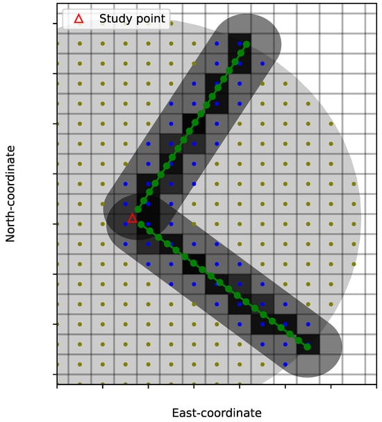
Figure 2.
For each study point (red triangle), the local horizon is calculated by generating radial rays at integer azimuths (green lines). Along the rays, the height is evaluated in evenly spaced points (green markers) and the elevation angles from the study point to each of the points are calculated. The heights along the rays are found from the DSM cells that the ray intersects (dark shaded cells). To reduce the number of lookups in the DSM that are necessary to find the heights, buffers are used to reduce the number of relevant DSM cells. First, a buffer is created around the study point to extract the first set of DSM cells to check (olive markers). Second, the final set to evaluate is found by selecting DSM cells within a thinner buffer created around the ray (blue markers). The width of the buffer around the study points is calculated by Equation (8), while the width of the buffers around the rays is set equal to two times the resolution of the grid.
A major challenge when computing the local horizons is to reduce the computation cost, especially when using a high-resolution DSM. The computational cost can be reduced considerably by ensuring a lookup against a DSM that is as small as possible. This can be performed by creating buffers around the road corridor, the study points, and the rays and then successively eliminating cells in the DSM outside the buffers.
The radii of the buffers surrounding the road corridors and the study points were determined by assuming a maximum elevation () for the area. Ignoring satellites with elevations smaller than a chosen cutoff angle (), the maximum search radius can be found by
where is the height of the study point [6]. The search radius was found by considering the geometry of a planar surface with height , and is the highest elevation above the surface. The radius defined by (8) is the smallest radius the buffer must have to ensure that all terrain points that could possibly block satellite signals are evaluated. As an example, with a cutoff angle of 10° and the highest elevation set to 350 m above the ellipsoid, the buffer should be at least 2000 m wide.
2.5. Calculation of DOP
The DOP is a function of diagonal elements of the cofactor matrix originating from a point positioning adjustment of pseudorange observations [24]. The design matrix () of the adjustment has as many rows as there are visible satellites, and the rows are defined by the unit line-of-sight vectors () and an extra column necessary for estimating the error of the receiver clock. The clock errors () are often estimated in length units (, where c is the speed of light), i.e., the additional column of the design matrix is set to unity.
From , the cofactor matrix is given:
Hence, the cofactor matrix is calculated from the line-of-sight vectors only, without the need for any pseudorange observations. From the diagonal elements of the cofactor matrix, different DOP indices can be calculated to assess, e.g., the accuracy in 3D position (PDOP), the horizontal and vertical positioning accuracy (HDOP and VDOP), or the full geometry (GDOP), see Table 3. Note that the HDOP in general is smaller than the PDOP because it does not include the cofactor of the vertical. The horizontal, vertical, and positioning accuracy follow by multiplying the DOP values by the measurement accuracy, if known [24].
Table 3.
DOP indices that can be calculated from the diagonal elements of the cofactor matrix .
To calculate , a minimum of four satellites in view is necessary. However, if several GNSS constellations are combined, it is necessary to estimate corrections to the broadcast offsets between the system time of GPS and the system time of the other constellations. This will reduce the degrees of freedom of the system of equations and increase the DOP. To ensure this effect, one more column vector can be included in for each extra constellation.
For a particular constellation (BeiDou, Galileo, or GLONASS), the elements of the column vector () are set to one for all rows in that include a line-of-sight vector to the current constellation. For other rows, the elements are set to zero. The expansion of with extra columns implies that one more satellite per extra constellation is needed for calculating .
3. Results
Three study areas were selected for the simulations, i.e., the southbound MODI corridor from Oslo to Svinesund Bridge at the Norwegian–Swedish border, Hamburg City, and the northbound MODI corridor from Rotterdam in the Netherlands to the Dutch–German border. The MODI corridors in the Netherlands and in Norway are characterized by rural highways surrounded by agricultural areas and low hills covered by woods. The city center of Hamburg is an urban area with road intersections, bridges, and buildings with up to fifteen stories. We believe that the three selected study areas appropriately represent the road types, terrain, and surroundings found in the MODI corridor and that the obtained results, therefore, may be of value also for similar road sections in other parts of the corridor. Along the road corridors, we defined multiple study points with spacing as listed in Table 4, but points in tunnels and under major road intersections were masked and not analyzed.
Table 4.
Key parameters for each study area.
For all study areas, six different combinations of constellations were investigated. They were as follows:
- GPS.
- GPS + BeiDou.
- GPS + Galileo.
- GPS + GLONASS.
- GPS + BeiDou + Galileo.
- GPS + BeiDou + Galileo + GLONASS (all four constellations).
Hence, the GPS constellation was included in all cases. Note that the constellation combining GPS and Galileo is relevant for the Galileo High Accuracy Service, providing corrections (orbits and clocks) and biases (code and phase) for Galileo and GPS signals [26]. A cutoff elevation angle of 10° was used, i.e., the satellites with the lowest elevations were not included in the simulations. We chose to focus on HDOP because horizontal positioning is the most relevant for navigation and positioning of vehicles, but we are aware that vertical accuracy may be vital for use-cases where traffic occurs on multiple levels, e.g., at highway overpasses [2].
The simulations were carried out on 3 April 2024, and to investigate the effect of different satellite geometries, HDOP was calculated for every 15 min throughout the day. This gives a total of 96 solutions for each combined constellation. Based on the 96 solutions, we calculated the median and maximum HDOP for each study point. The median is the HDOP that should be expected for a particular study point, while the maximum should be considered as a worst case that occasionally may arise.
Figure 3, Figure 4 and Figure 5 illustrate the maximum HDOP for the three study areas, and Table 5 lists the percentages of study points that have median and maximum HDOP in the range of DOP classes adopted from [27], i.e., HDOP better than 2 is considered as excellent, 2–5 is good, 5–10 is average, 10–20 is weak, and higher than 20 is poor. For the three subsections of the MODI corridor, 99–100% of the study points have a median HDOP categorized as excellent or good regardless of which constellation is used. Also, the maximum HDOP is for the majority of the study points excellent or good (88–100%). This suggests that the overall GNSS performance for the MODI corridor is good. However, high percentages of study points with good or excellent median and maximum HDOP do not rule out that some areas may have challenging GNSS performance during parts of the day. This applies first of all to the corridor in Hamburg and partly also to Norway.
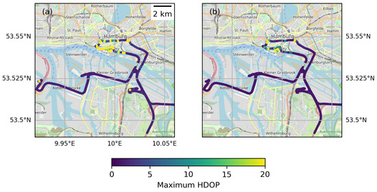
Figure 3.
Maximum horizontal dilution of precision (HDOP) along the MODI corridor in Hamburg City, Germany, using GPS only (a) and GPS combined with Galileo (b). The yellow and green dots indicate high maximum HDOP and can mainly be attributed to tall buildings hampering satellite visibility. Basemap from OpenStreetMap [3].
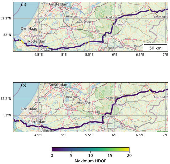
Figure 4.
Maximum horizontal dilution of precision (HDOP) along the MODI corridor from Rotterdam to the Dutch–German border using GPS only (a) and GPS combined with Galileo (b). The yellow dots indicate high maximum HDOP and can be attributed to trees next to the highway hampering satellite visibility. Basemap from OpenStreetMap [3].
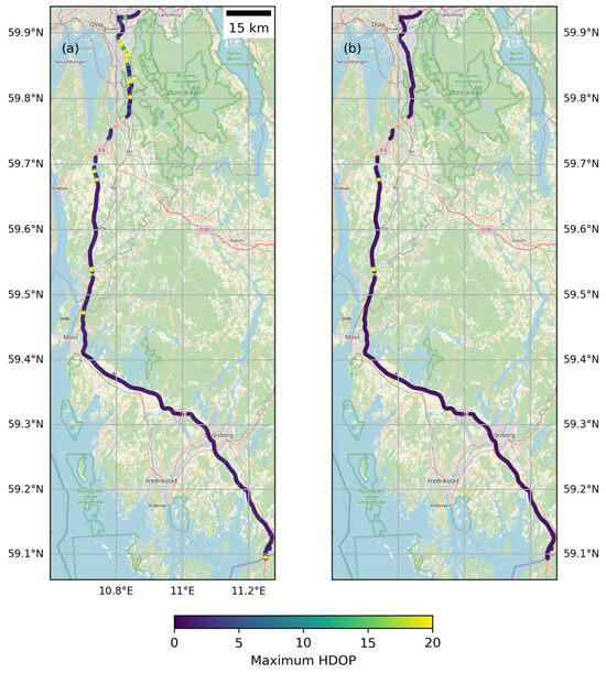
Figure 5.
Maximum horizontal dilution of precision (HDOP) along the MODI corridor from Oslo to Svinesund Bridge, Norway, using GPS only (a) and GPS combined with Galileo (b). The yellow and green dots indicate high maximum HDOP and can be attributed to trees and steep rock cuttings close to the road hampering satellite visibility. Basemap from OpenStreetMap [3].
Table 5.
Percentages of points with median/maximum HDOP in different HDOP classes. The simulations in Hamburg were performed with both a 1 m and a 10 m DSM.
In Hamburg, the challenging study points are concentrated in HafenCity, characterized by streets surrounded by tall buildings. With GPS only, 8% of the study points have a weak or poor maximum HDOP. For HafenCity, we therefore also calculated the availability of the system, see Figure 6. The availability is here defined as the percentage of the 96 solutions that have HDOP smaller than a threshold of five (excellent and good). Hence, we assume that HDOP better than five implies enough well-distributed satellites for accurate positioning and navigation. In the HafenCity, there are study points where the system is available as little as 5% of the time if GPS is the only constellation. This suggests that there are areas in Hamburg where users that rely on GPS should expect that positioning is not possible at certain times of the day and that the achieved position is not reliable. With two constellations in combination, the availability of the system increases significantly, and when all constellations are combined, the system is available more than 95% of the time for 99% of the study points also in Hamburg.
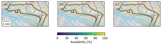
Figure 6.
Availability of GNSS (in percent) in a challenging part of the city center of Hamburg. Availability is here the percentage of study epochs that have excellent or good HDOP (<5). (a) shows the availability with GPS only, (b) with GPS combined with Galileo, and (c) with all constellations. Basemap from OpenStreetMap [3].
To investigate whether it is possible to avoid high HDOP for certain periods of the day, we plotted HDOP time series throughout the day at the ten locations with the lowest system availability (see Figure 7). For all cases, the HDOP is very high (up to 100) for several epochs, and there are also epochs for which it was not possible to compute the HDOP. When GPS is combined with Galileo, system availability increases significantly, and the number of epochs without an HDOP value decreases. Still, the system is not available simultaneously at all points for any of the 96 epochs. This implies that with GPS only or GPS combined with Galileo, it is not possible to avoid large HDOP by visiting HafenCity at a specific time of the day. This changes when all constellations are combined. In that scenario, the system is available at 38% of the epochs, and longer slots exist where the system is available at most locations.
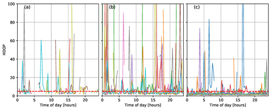
Figure 7.
Time series of HDOP at the 10 locations (colors represent time series from different locations) with lowest system availability in Hamburg HafenCity with GPS only (a), GPS in combination with Galileo (b), and with all constellations (c). The red dashed line indicates the threshold for system availability, i.e., HDOP < 5.
Our results clearly demonstrate the advantage of combining several constellations in urban areas. With GPS only, the mean number of available satellites is 8 in Hamburg while the mean is 19, 14, and 15 when GPS is combined with BeiDou, Galileo, and GLONASS, respectively. It is noticeable that the percentage of excellent study points is larger when GPS is combined with BeiDou compared to GPS combined with Galileo or GLONASS. This is because the BeiDou constellation has more satellites than the Galileo and GLONASS constellations (51 satellites for BeiDou vs. 27 and 24 satellites for Galileo and GLONASS, respectively, as of June 2025).
In Norway, most of the challenging study points are in an area south of Oslo where nearby trees and steep rock cuttings next to the highway hamper satellite visibility. Also, for a small group of study points close to Rotterdam in the Netherlands, trees next to the highway create high simulated HDOP. Inspecting the DSM and using photos from Google Streetview, we found that the trees create cells in the DSM that are 10 to 15 m higher than the highway itself. This results in local horizons with an elevation of about 55°. While rock cuttings block GNSS signals completely, it is likely that the trees cause the most severe problems for carrier-phase measurements and precise applications of GNSS where decimeter, or even centimeter, accuracy is required. This is because trees and other types of vegetation often create cycle slips, which are critical for carrier-phase measurements but do not influence pseudoranges that are more robust to vegetation [28]. For code-based measurements based on pseudoranges, navigation will often be possible since most trees do not block the GNSS signals completely. A weakness with our methodology, using DSMs to assess the visibility of the satellites, is that we are not able to represent canopy geometries accurately and distinguish between massive obstacles that block the GNSS signals completely and signal fading of satellites close to permeable objects like trees. Although not tested in the present study, we suggest using canopy masks to separate trees from the DSM when effects of trees are not wanted in simulations. Also, in the Netherlands and in Norway, the simulations indicate that improved GNSS performance may be obtained by combining several constellations; with all constellations combined, 100% of the study points have excellent maximum HDOP.
We were not able to identify any relation between the simulated HDOP and the direction of the streets in the study areas. This is an effect we had expected to observe, since GNSS satellites typically reach higher elevation to the east, west, and south compared to the north. The impact is that GNSS visibility along roads in the east–west direction should be more prone to obstacles than roads in the south–north direction. A similar effect was reported by [10], who found that the accuracy decreased especially on the southwest and southeast sides of buildings. However, no such pattern was observed in the simulated DOP. We suggest that it is likely that such an effect will be more pronounced at higher latitudes where GNSS satellites in general reach lower elevations than along the MODI corridor.
4. Discussion
4.1. Comparison to HDOP from In Situ Measurements
To validate the methodology and computer code used to calculate DOP and satellite visibility, we compared the simulations with in situ GNSS measurements from the city center of Hamburg. The GNSS measurements were collected from a survey vehicle traveling along the MODI corridor at 30. March 2024 between 06.00 and 07:50 CET, and a setup of two receivers was used. The Sony CXD5610GF is a low-cost and small-size receiver that provides GNSS standalone solutions only, while the u-blox EVK-M8U has internal Micro-Electro-Mechanical Systems (MEMS) sensors which offer untethered dead reckoning navigation. Both receivers were connected to a common roof-mounted Maxtena MEA-1400-MM antenna. The Sony receiver was configured to track a combined constellation of GPS and Galileo, while the u-blox receiver tracked GPS and GLONASS satellites.
The receivers were configured with a sampling interval of 1 s. These data were thinned to include only one study point for every 50 m. By thinning the data, we obtained evenly spaced data along the road corridor, and we also removed multiple observation epochs from locations where the survey vehicle stopped or traveled slowly. An elevation cutoff angle of 5° was used both when collecting the data and in the simulations. To imitate a roof-mounted antenna, the study points in the simulations were elevated by 1.5 m above the ground level given by the DSM.
Initial comparison indicated a low correlation between simulations and observations from the Sony receiver. Furthermore, the observed HDOP showed small variations along the road corridor and only a modest increase in areas flagged as challenging by the simulations. Closer inspection of the data revealed that the receiver in some study points tracked more than double the number of satellites found to be above the horizon by simulations. This explains the lower HDOP, and our first suspicion was that the simulations were inaccurate due to a DSM that does not represent the local horizon properly. However, we compared the calculated horizon for some challenging study points to photos from Google Streetview, and it appears that the calculated horizons are credible. At the same time, it is well-known that GNSS receivers are able to receive reflected or refracted signals from NLOS satellites [29,30], which in severe conditions may result in errors larger than 1 km [31]. Reception of NLOS signals is especially relevant in urban areas where, e.g., building facades, windows, wet asphalt, and parked vehicles are potential reflectors and may lead to NLOS signals with strength comparable to line-of-sight signals but with large pseudorange errors. As multipath signals arise together with the direct signal from the satellite, the NLOS signal originates from one or more reflectors when the direct signal is blocked [29]. NLOS signals may therefore be more difficult to detect than multipath signals and are therefore a major source of degraded positioning accuracy in urban areas [8,30]. With respect to the DOP registered by the receiver, the presence of NLOS signals will paradoxically result in a decrease in DOP because the receiver interprets NLOS satellites as being within the line of sight. Hence, the receiver does not take into account signal quality or the altered signal path due to reflections when calculating DOP.
Unfortunately, the Sony receiver’s ability to track NLOS satellites makes the data set not well suited to assess our simulations. Still, we tentatively tried to identify and exclude the NLOS satellites from the HDOP calculations by using logged signal-to-noise ratios (SNRs). We remark that an NLOS classifier based on SNR thresholding alone can usually not distinguish flawlessly between LOS and NLOS signals and the SNR should, when available, be used together with other GNSS quality indicators like, e.g., the standard deviation of the pseudorange and the pseudorange residual [30,32]. Nevertheless, signals with low SNR are more likely to originate from NLOS satellites than signals with a high SNR [32], and previous studies suggest that an SNR smaller than 30–35 dB indicates signal reception from NLOS satellites [8,32].
For Hamburg City, we investigated SNR thresholds between 25 and 40 dB, and the highest percentage of correct predictions (True Positive and True Negative; True Positive is when the classifier predicts the positive category (LOS) correctly and True Negative is when the classifier predicts the negative category (NLOS) correctly) was obtained when the SNR threshold was set to 30 dB. With this threshold, 90.0% of in total 17,235 pseudoranges were correctly predicted as LOS or NLOS (see Figure 8). Furthermore, a quite low percentage (6.7%) of NLOS observations were misclassified as LOS (False Positive, which is when the classifier predicts the positive category (LOS) incorrectly). We consider the obtained result to be quite good, and it is comparable to results obtained by using more quality indicators and machine learning algorithms [30,32]. With most NLOS satellites eliminated, we obtained a correlation of 0.82 between the number of LOS satellites tracked by the receiver and the number of satellites found to be above the local horizon by simulations. Furthermore, the correlation between observed and simulated HDOP increased from −0.19 to 0.24. The significant increase in correlation suggests that the Sony receiver’s ability to track NLOS satellites is an important explanation for the initially found low correlation between observed and simulated HDOP.
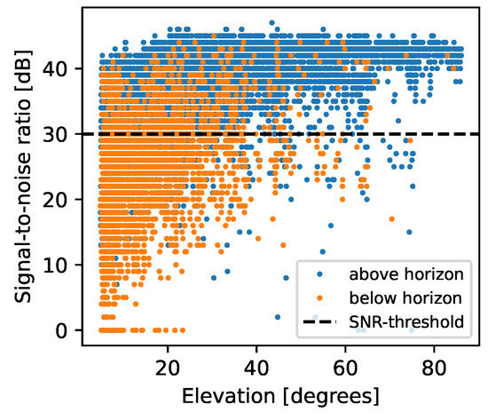
Figure 8.
Signal-to-noise ratios (SNRs) of observations to satellites above (blue) and below (orange) the horizon. The dashed line indicates 30 dB, which was used as threshold for classifying line-of-sight (LOS) and non-line-of-sight (NLOS) observations. Blue markers above the threshold and orange markers below the threshold indicate correct predictions based on SNR.
Compared to the Sony receiver, the u-blox receiver appears more conservative with respect to which satellites to include in its solutions. This makes the u-blox data more suitable for validating our simulations. Figure 9 shows differences between the observations and the simulations in Hamburg. In general, the HDOP differences are small, i.e., the absolute values of the differences are mostly less than 0.5, and they have a standard deviation of 0.35. Some larger negative differences can still be identified. The largest differences are typically found in streets flanked by tall buildings, e.g., in Hamburg HafenCity, and they correspond to points where the u-blox receiver tracks more satellites than found to be above the local horizon in the simulations. Interestingly, there are also areas where the simulations indicate more satellites above the horizon than tracked by the u-blox receiver, e.g., in the southwestern part of the study area. A possible explanation is missing objects in the DSM. However, the HDOP differences are less than one in these study points, and it appears that the extra satellites have minor effects on the simulated HDOP.
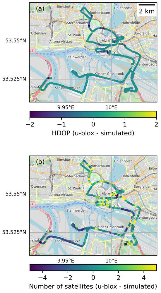
Figure 9.
Differences between HDOP (a) and number of visible satellites (b) observed by the u-blox receiver and calculated by simulations in Hamburg City. To make the figure easier to interpret, only every second study point is plotted. Basemap from OpenStreetMap [3].
The fact that there are study points where the u-blox tracks more satellites than found to be above the local horizon by the simulations suggests that the u-blox receiver also includes NLOS satellites in its solutions. Other possible explanations of larger differences are errors and inaccuracies in the DSM that may arise because the DSM is a snapshot of the Earth’s surface at the moment of data collection. For instance, objects may exist that are not part of the DSM, and vice versa. This is most relevant in urban environments where anthropogenic changes arise frequently. Furthermore, it is not possible from the DSM alone to distinguish between massive constructions that will block the GNSS signals completely and permeable objects that allow the GNSS signals to pass. This applies to, e.g., a group of study points on the western side of the bridge Neue Elbbrücke, crossing the river Norderelbe at approximately 10.026° E, 53.532° N, for which up to seven more satellites are included in the u-blox solutions. The middle of the bridge is made of trusses which in the simulation appear as a massive construction and block most satellites to the east and southeast (see Figure 10). In reality, it is plausible that the GNSS signals may pass through the construction, as also indicated by the quite high number of satellites tracked by the u-blox receiver. It is, however, possible that the signals passing through the trusses are refracted and deteriorated and not suitable for high-accuracy positioning.
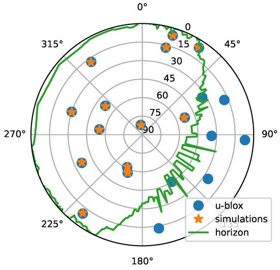
Figure 10.
Skyplot of satellite positions (observed and simulated) and the local horizon for a study point at the bridge Neue Elbbrücke crossing Norderelbe in Hamburg, Germany, at approximately 10.026° E, 53.532° N. The fringes in the local horizon are created by trusses on the bridge that partly block satellite visibility to the east and southeast. Only satellites with an elevation angle larger than 5° are shown.
4.2. Effect of Spatial Resolution of DSM
To address the effect of the DSM’s spatial resolution on the simulations, we calculated HDOP in Hamburg using also a 10 m DSM. Figure 11 shows local horizons surrounding two study points in Hamburg HafenCity calculated with both a 1 m and 10 m DSM. Using a coarser-resolution DSM offers significant advantages in terms of computational costs and memory requirements. For Hamburg, we evaluated all cells in the DSM within a radius of 500 m from the study points, which implied evaluating 782,135 and 7827 cells with a 1 m and 10 m DSM, respectively. Using a 10 m DSM reduced the computational time by a factor of 12 compared to using a 1 m DSM.
Figure 11.
Skyplots of local horizons calculated with a 1 m (blue) and 10 m (orange) DSM at (a) Am Sandtorkai (9.986501° E, 53.542885° N) and (b) Osakaallee (9.999312° E, 53.541725° N) in Hamburg HafenCity. Green stars and red dots indicate locations of GPS and Galileo satellites, respectively, on 30 March 2024 06:09:48 UTC. Only satellites with an elevation angle larger than 10° are shown.
As expected, the one-meter-resolution DSM reveals more small details at the two example points. The first point, located at Am Sandtorkai (9.986501° E, 53.542885° N), is in a narrow street heading east–west, flanked by concrete buildings on both sides. Here, the ten-meter-resolution DSM adequately captures the horizon depicted by the one-meter DSM. The second example point, situated in a north–south-heading street (Osakaallee at 9.999312° E, 53.541725° N), has a more diverse environment. The southwest features a standard seven-story building, with a smaller four-story building to the northeast and a narrow fifteen-story high-rise building to the northwest. In such complex surroundings, there are significant differences between the two DSMs. Compared to the 1 m DSM, the 10 m DSM captures the key elements of the local horizon, but it appears to be too coarse to provide an accurate representation of the local horizon. At this particular study point, the lower skyplot in Figure 11 shows that this will be critical for determining the visibility of four of the satellites in a combined constellation of GPS and Galileo.
We calculated the percentages of study points falling within each of the five HDOP classes (median and maximum values) also with the 10 m DSM. Table 5 shows that similar results were obtained with the 10 m as with the 1 m DSM, i.e., most study points have excellent or good median HDOP values, but there are some points where the maximum HDOP suggests weak or poor GNSS performance. This is also evident from Figure 12, where the simulations using the 10 m DSM pinpoint to a large extent the same problematic areas as those identified with the 1 m DSM. To quantify the similarity, we calculated the correlations between the 1 m and 10 m solutions. These correlations varied depending on the constellation used, ranging from 0.72 to 0.86 for the median HDOP and between 0.51 and 0.87 for the maximum HDOP. Interestingly, the strongest correlation was for the median HDOP when only GPS was employed, whereas the maximum HDOP showed the highest correlation when all constellations were combined.
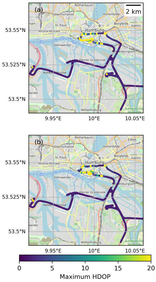
Figure 12.
Maximum horizontal dilution of precision (HDOP) along the MODI corridor in Hamburg City, Germany, calculated with a 1 m DSM (a) and a 10 m DSM (b). To make the figures easier to interpret, only every second study point is plotted. Basemap from OpenStreetMap [3].
The obtained results propose that a 10 m DSM provides a sufficiently accurate representation of the local horizon when aiming at identifying challenging areas with a view to GNSS visibility. However, for a more precise analysis at complex urban study points, a DSM with a higher spatial resolution is desirable, as it will provide more accurate and reliable information.
5. Conclusions
We simulated DOP and satellite visibility in three subsections (Oslo to Svinesund Bridge at the Norwegian–Swedish border, Hamburg City, Germany, and the northbound highway from Rotterdam to the Dutch–German border) of the MODI project road corridor by using GNSS almanacs and high-resolution DSMs. The aim of this study was to demonstrate that simulations can be useful for identifying challenging areas with a view to GNSS performance. GNSS performance may be critical when GNSS provides information to systems used for navigation, position determination, automated mobility, and advanced driver-assist systems. Maps with simulated DOP values may be used for route planning and to predict whether remaining satellites in challenging areas provide a strong enough constellation for reliable positioning. Furthermore, DOP simulations can provide insights into the causes of local signal outages, and road administrators can leverage DOP maps to pinpoint specific areas where the clearing of trees and vegetation would enhance safe navigation and facilitate reliable GNSS-supported autonomous driving and transportation systems.
In our study, we focused on the HDOP, as the horizontal dimension is the most important for navigation and driver assistance systems. The simulations indicate that the overall satellite visibility and HDOP are excellent or good in the three study areas. However, there are also smaller areas where users, especially those who rely on the GPS constellation alone, should expect degraded positioning accuracy or even system failure. The challenging areas are first of all found in urban areas where buildings close to the road hamper visibility for low-elevation satellites. In addition, we identified smaller areas at highways where nearby trees and steep rock cuttings increase the HDOP. Combining GPS with one or several other GNSS constellations improves the availability of satellites and reduces the simulated HDOP in the challenging areas significantly. In interpreting the results, it is important to remember that high DOP almost always indicates challenging GNSS conditions, while low DOP does not necessarily imply high positioning accuracy.
To assess the data sets and applied methods, we also compared our simulations with HDOP calculated from in situ observations collected with a low-cost Sony receiver and a u-blox receiver with internal MEMS sensors. The correlation between HDOP values obtained from simulations and values registered by the Sony receiver was unexpectedly low, while we found reasonable agreement between simulations and values registered by the u-blox receiver. Hence, the obtained results were strongly dependent on the receiver in play. The low correlation between simulations and the Sony receiver arises due to the receiver’s ability to track reflected signals from NLOS satellites, i.e., satellites with elevations lower than the local horizon. Because the receivers also use NLOS satellites to compute positions, the HDOP calculated by the receiver will differ from the simulations that include only satellites above the local horizon. Reducing the number of NLOS satellites in the receiver’s solution by SNR thresholding increased the correlations significantly and led to results that agree reasonably also for the Sony receiver. This shows that the HDOP values obtained in our simulations are conservative compared to HDOP derived from in situ observations. At the same time, it is important to be aware that the carrier phase of NLOS signals may change significantly and that NLOS observations may corrupt positioning based on carrier-phase measurements if not eliminated from the solution. We therefore suggest that simulated HDOP is most relevant for high-precision applications based on carrier-phase measurements.
Major advantages of simulations over in situ observations are that simulated DOP is independent of receiver setup and performance, and simulations can be performed for any epoch, elevation mask, and combination of GNSS constellations. Moreover, simulations are cost-effective and an environmentally friendly alternative to collecting data from a survey vehicle. The disadvantages are errors in the terrain elevation data and that it is complex to model real-life effects of reflected signals, multipath signals, reception of signals through non-line-of-sight paths, and signal diffraction. Given the significant impact of construction and demolition on the local horizon, using updated DSMs is critical for reliable DOP simulations.
Author Contributions
Conceptualization, K.B. and C.W.L.; methodology, K.B. and C.W.L.; software, K.B.; validation, K.B.; formal analysis, K.B.; investigation, K.B.; data curation, K.B. and C.W.L.; writing—original draft preparation, K.B.; writing—review and editing, K.B. and C.W.L.; visualization, K.B. All authors have read and agreed to the published version of the manuscript.
Funding
This research was accomplished as part of the MODI project (Project number: 101076810), funded by the European Union’s program Horizon Europe. Views and opinions expressed are, however, those of the authors only and do not necessarily reflect those of the European Union or CINEA. Neither the European Union nor the granting authority can be held responsible for them.
Institutional Review Board Statement
Not applicable.
Informed Consent Statement
Not applicable.
Data Availability Statement
The raw data supporting the conclusions of this article are cited in the text. Data sets derived from the raw data and presented in this study are available on reasonable request from the corresponding author.
Acknowledgments
The authors would like to acknowledge the open-access policy of MetadatenVerbund, Actueel Hoogtebestand Nederland, and the Norwegian Mapping Authority, who provided the DSMs. All maps were made with the cartographic Python library, Cartopy, developed by Met Office, UK. The authors are indebted to three anonymous reviewers for valuable comments that helped improve the manuscript.
Conflicts of Interest
The authors declare no conflicts of interest. The funders had no role in the design of the study; in the collection, analyses, or interpretation of data; in the writing of the manuscript; or in the decision to publish the results.
Abbreviations
The following abbreviations are used in this manuscript:
| AHN | Actueel Hoogtebestand Nederland |
| CCAM | Cooperative, Connected, and Automated Mobility |
| CET | Central European Time |
| DAP | Digital Aerial Photogrammetry |
| DSM | Digital Surface Model |
| DTM | Digital Terrain Model |
| EPSG | European Petroleum Survey Group |
| GDOP | Geometrical Dilution of Precision |
| GLONASS | GLObalnaya NAvigatsionnaya Sputnikovaya Sistema |
| EVRF | European Vertical Reference Frame |
| GNSS | Global Navigation Satellite System |
| GPS | Global Positioning System |
| DOP | Dilution of Precision |
| HDOP | Horizontal Dilution of Precision |
| lidar | Light detection and ranging |
| LOS | Line of sight |
| NLOS | Non-line of sight |
| MEMS | Micro-Electro-Mechanical Systems |
| PDOP | Position Dilution of Precision |
| RMSE | Root Mean Square Error |
| SNR | Signal-to-noise ratio |
| SPP | Single Point Positioning |
| VDOP | Vertical Dilution of Precision |
| UTM | Universal Transverse Mercator |
References
- European Commission. MODI A leap towards driving automation level 4 features. In Towards Cooperative, Connected and Automated Mobility—Contributions of Horizon Europe Projects Managed by CINEA; European Climate, Infrastructure and Environment Executive Agency, European Union: Brussels, Belgium, 2023; ISBN 978-92-95231-50-4. Available online: https://data.europa.eu/doi/10.2926/686283 (accessed on 1 June 2025).
- Arnesen, P.; Brunes, M.T.; Schiess, S.; Seter, H.; Södersten, C.J.H.; Bjørge, N.M.; Skjæveland, A. TEAPOT. Summarizing the Main Findings of Work Package 1 and Work Package 2; Technical Report 2022:00170; SINTEF: Trondheim, Norway, 2022; ISBN 978-82-1407546-5. [Google Scholar]
- OpenStreetMap Contributors. Planet Dump. 2025. Available online: https://planet.osm.org (accessed on 1 June 2025).
- Schiess, S.; Berget, G.E.; Arnesen, P.; Brunes, M.T.; Seter, H.; Muggerud, A.M.F. GNSS Technology for Precise Positioning in CCAM: A Comparative Evaluation of Services. IEEE Access 2023, 11, 47816–47826. [Google Scholar] [CrossRef]
- Langley, R.B. Dilution of Precision. GPS World 1999, 10, 52–59. [Google Scholar]
- Gandolfi, S.; La Via, L. SKYPLOT_DEM: A tool for GNSS planning and simulations. Appl. Geomat. 2011, 3, 35–48. [Google Scholar] [CrossRef]
- Ruwisch, F.; Schön, S. GNSS Feature Map Aided RTK Positioning in Urban Trenches. In Proceedings of the IEEE 26th International Conference on Intelligent Transportation Systems (ITSC), Bilbao, Spain, 24–28 September 2023; pp. 5798–5804. [Google Scholar] [CrossRef]
- Hsu, L.T.; Gu, Y.; Kamijo, S. NLOS Correction/Exclusion for GNSS Measurement Using RAIM and City Building Models. Sensors 2015, 15, 17329–17349. [Google Scholar] [CrossRef] [PubMed]
- Wang, L.; Groves, P.D.; Ziebart, M.K. Multi-constellation GNSS performance evaluation for urban canyons using large virtual reality city models. J. Navig. 2012, 65, 459–476. [Google Scholar] [CrossRef]
- Kleijer, F.; Odijk, D.; Verbree, E. Prediction of GNSS Availability and Accuracy in Urban Environments Case Study Schiphol Airport. In Location Based Services and TeleCartography II: From Sensor Fusion to Context Models; Gartner, G., Rehrl, K., Eds.; Springer: Berlin/Heidelberg, Germany, 2009; pp. 387–406. ISBN 978-3-540-87393-8. [Google Scholar] [CrossRef]
- Kaplan, E.D.; Hegarty, C. Understanding GPS/GNSS: Principles and Applications; Artech House Publishers: Norwood, MA, USA, 2017; ISBN 9781630810580. [Google Scholar]
- Reid, T.G.R.; Houts, S.E.; Cammarata, R.; Mills, G.; Agarwal, S.; Vora, A.; Pandey, G. Localization Requirements for Autonomous Vehicles. SAE Int. J. Connect. Autom. Veh. 2019, 2, 173–190. [Google Scholar] [CrossRef]
- Thitipatanapong, R.; Wuttimanop, P.; Chantranuwathana, S.; Klongnaivai, S.; Boonporm, P.; Noomwongs, N. Vehicle Safety Monitoring System with Next Generation Satellite Navigation: Part 1 Lateral Acceleration Estimation. SAE Technical Paper 2015-01-012. Available online: https://doi.org/10.4271/2015-01-0123 (accessed on 1 June 2025).
- Melendez-Pastor, C.; Ruiz-Gonzalez, R.; Gomez-Gil, J. A data fusion system of GNSS data and on-vehicle sensors data for improving car positioning precision in urban environments. Expert Syst. Appl. 2017, 80, 28–38. [Google Scholar] [CrossRef]
- Yeong, D.; Velasco-Hernandez, G.; Barry, J.; Walsh, J. Sensor and Sensor Fusion Technology in Autonomous Vehicles: A Review. Sensors 2021, 21, 2140. [Google Scholar] [CrossRef] [PubMed]
- Breili, K.; Simpson, M.J.R.; Klokkervold, E.; Ravndal, O.R. High-accuracy coastal flood mapping for Norway using lidar data. Nat. Hazards Earth Syst. Sci. 2020, 20, 673–694. [Google Scholar] [CrossRef]
- Yastikli, N.; Bayraktar, H.; Erisir, Z. Performance Validation of High Resolution Digital Surface Models Generated by Dense Image Matching with the Aerial Images. Int. Arch. Photogramm. 2014, 40, 429–433. [Google Scholar] [CrossRef]
- Gruen, A. Development and status of image matching in photogrammetry. Photogramm. Rec. 2012, 27, 36–57. [Google Scholar] [CrossRef]
- Goodbody, T.R.H.; Coops, N.C.; White, J.C. Digital Aerial Photogrammetry for Updating Area-Based Forest Inventories: A Review of Opportunities, Challenges, and Future Directions. Curr. For. Rep. 2019, 5, 55–75. [Google Scholar] [CrossRef]
- Denker, H. A new European gravimetric (quasi)geoid EGG2015, 2015. In Proceedings of the IUGG 2015, Prague, Czech Republic, 22 June–2 July 2015. [Google Scholar]
- Ågren, J.; Strykowski, G.; Bilker-Koivula, M.; Omang, O.; Märdla, S.; Forsberg, R.; Ellmann, A.; Oja, T.; Liepins, I.; Parseliunas, E.; et al. The NKG2015 gravimetric geoid model for the Nordic-Baltic region. In Proceedings of the 1st Joint Commission 2 and IGFS Meeting International Symposium on Gravity, Geoid and Height Systems, Thessaloniki, Greece, 19–23 September 2016. [Google Scholar] [CrossRef]
- Ma, L.; Zhou, S. Positional Accuracy of GPS Satellite Almanac. Artif. Satell. 2014, 49, 225–231. [Google Scholar] [CrossRef]
- Wang, J.; Morell, J.; Morton, Y. Predicting GLONASS satellite orbit based on an almanac conversion algorithm for controlled ionosphere scintillation experiment planning. In Proceedings of the 24th International Technical Meeting of the Satellite Division of The Institute of Navigation (ION GNSS 2011), Portland, OR, USA, 20–23 September 2011; pp. 3118–3124. [Google Scholar]
- Leick, A. GPS Satellite Surveying, 3rd ed.; John Wiley & Sons, Inc.: Hoboken, NJ, USA, 2004; ISBN 0-471-05930-7. [Google Scholar]
- Torge, W.; Müller, J. Geodesy, 4th ed.; Walter de Gruyter: Berlin, Germany, 2012; ISBN 978-3-11-020718-7. [Google Scholar]
- Fernandez-Hernandez, I.; Chamorro-Moreno, A.; Cancela-Diaz, S.; Calle-Calle, J.D.; Zoccarato, P.; Blonski, D.; Senni, T.; de Blas, F.J.; Hernández, C.; Simón, J.; et al. Galileo high accuracy service: Initial definition and performance. GPS Solut. 2022, 26, 65. [Google Scholar] [CrossRef]
- Duchoň, F.; Hanzel, J.; Babinec, A.; Rodina, J.; Pásztó, P.; Gajdošík, D. Improved GNSS localization with the use of DOP parameter. Appl. Mech. Mater. 2014, 611, 450–466. [Google Scholar] [CrossRef]
- Andersen, H.E.; Strunk, J.; McGaughey, R.J. Using High-Performance Global Navigation Satellite System Technology to Improve Forest Inventory and Analysis Plot Coordinates in the Pacific Region; Technical Report PNW-GTR-1000; Pacific Northwest Research Station, U. S. Department of Agriculture: Olympia, WA, USA, 2022. [Google Scholar]
- Petovello, M.; Groves, P.D. Multipath vs. NLOS signals. Inside GNSS 2013, 8, 40–44. [Google Scholar]
- Li, L.; Elhajj, M.; Feng, Y.; Ochieng, W.Y. Machine learning based GNSS signal classification and weighting scheme design in the built environment: A comparative experiment. Satell. Navig. 2023, 4, 12. [Google Scholar] [CrossRef]
- Zidan, J.; Adegoke, E.I.; Kampert, E.; Birrell, S.A.; Ford, C.R.; Higgins, M.D. GNSS Vulnerabilities and Existing Solutions: A Review of the Literature. IEEE Access 2021, 9, 153960–153976. [Google Scholar] [CrossRef]
- Xu, H.; Angrisano, A.; Gaglione, S.; Hsu, L.T. Machine learning based LOS/NLOS classifier and robust estimator for GNSS shadow matching. Satell. Navig. 2020, 1, 15. [Google Scholar] [CrossRef]
Disclaimer/Publisher’s Note: The statements, opinions and data contained in all publications are solely those of the individual author(s) and contributor(s) and not of MDPI and/or the editor(s). MDPI and/or the editor(s) disclaim responsibility for any injury to people or property resulting from any ideas, methods, instructions or products referred to in the content. |
© 2025 by the authors. Licensee MDPI, Basel, Switzerland. This article is an open access article distributed under the terms and conditions of the Creative Commons Attribution (CC BY) license (https://creativecommons.org/licenses/by/4.0/).