Thermal Analysis of a Turbulent Ventilated Cavity with Internal Heat Generation

Abstract

This work investigates heat transfer experimentally and numerically within a ventilated cavity, both with and without an internal heat source, simulating a room with a person at the interior at 1:3 scale. This setup has applications in building energy systems, cooling of electronic equipment, solar energy collectors, etc. The experimental configuration consists of a cube in which the left vertical wall is subjected to a uniform heat flux, and the opposing wall is maintained at a constant temperature. A rectangular parallelepiped heat source was placed inside. The remaining walls are thermally insulated, and air is the thermal fluid. Air enters and exits through square ports on the top surface. Experimental temperature profiles were recorded at multiple depths and heights. Corresponding numerical results for temperature fields, flow patterns, turbulent viscosity, and turbulent kinetic energy were generated using the Ansys Fluent 18 CFD software, with six turbulence models assessed against experimental data under steady-state conditions. A key finding is that the Nusselt number and the convective heat transfer coefficients (average) for the hot wall remain negligibly affected by the incorporation or status (on/off) of a heat source at the interior of the cavity, the biggest temperature difference (experimental vs numerical) corresponds to the rkε model with 6.2% when there is no thermal source in the cavity and the lowest difference for the average convective heat transfer coefficient is with the rslrso model with 5.2%.

1. Introduction

The sustained growth in energy use in arid regions, often attributed to mechanical ventilation, carries a substantial ecological cost. Given that most global electricity is generated from fossil fuels, this trend results in considerable atmospheric emissions of greenhouse gases, especially carbon dioxide [1]. Therefore, research into building ventilation has become critically urgent; indeed, to mitigate energy consumption, it must be considered an essential discipline.

The temperature and air velocity in a room are critical factors for occupant comfort. These conditions are disrupted by heat generated from people and electronics, which creates complex airflow and temperature patterns. Analyzing these effects is essential for optimizing ventilation systems and minimizing their electricity use. A cavity model provides an effective method for this analysis, offering control over the parameters used to understand heat transfer. In this study, a 1:3-scale cavity is used. Moreover, by validating the mathematical model with experimental data, we can accurately predict the system’s performance under a range of ambient conditions.

The literature on heat transfer in ventilated cavities, which may be related to rooms or offices, can be organized into two categories: (a) studies without internal heat generation and (b) studies with internal heat generation.

(a) Studies in cavities with ventilation and without heat generation at the interior:

A numerical study by Singh and Sharif [2] on mixed convective cooling in a ventilated, two-dimensional rectangular cavity examined the effect of air injection points on the hot and cold walls. Their analysis, which included isotherms, streamlines, and Nusselt numbers, showed that the maximum cooling effectiveness is achieved when the inlet is located near the bottom of the cold wall and the outlet near the top of the hot wall. Meanwhile, Posner et al. [3] focused on validating CFD models for indoor airflow. Using laser Doppler anemometry (LDA) and particle image velocimetry (PIV) in a scaled model room, they compared measurements against predictions from laminar, k-ε, and RNG k-ε models. They concluded that all three models accurately predicted flow trends, with simulation errors not exceeding 20%. Moraga and Lopez [4] conducted 3D numerical simulations of mixed convection in an air-cooled cavity, demonstrating that a 3D model is essential for accurately capturing the fluid mechanics and calculating the global Nusselt number, unlike simplified 2D approaches. In a complementary experimental study, Haslavsky et al. [5] investigated the interaction between mixing and displacement ventilation modes in a naturally ventilated enclosure with upper- and lower-sidewall openings. They found that the neutral plane’s height at the superior outlet (the plane separating inflow from outflow) decreased as the proportion of the lower to the upper vent heights (and areas) increased.

Rahman et al. [6] numerically investigated mixed convection in a vented enclosure, analyzing how the position of an inlet on the left wall (with a fixed outlet on the right) affected flow patterns, thermal distributions, and the average Nusselt number on the hot wall. In a study on natural ventilation, Daghigh et al. [7] quantified the influence of air exchange rate (ACH) and effectiveness (AEE) on thermal comfort (PMV) in an office, deriving linear regression models to describe these relationships. Further exploring natural convection, Raji et al. [8] identified a maximum interaction between forced and natural convection mechanisms and the existence of distinct flow regimes in a ventilated cavity. Complementing these numerical studies, Tanny et al. [9] experimentally characterized the average and turbulent air circulation across a vertically oriented opening in a floatability-driven enclosure, observing an airflow inclination due to buoyancy effects.

Saha et al. [10] numerically analyzed mixed convection in a 2D cavity with a heated vertical wall, demonstrating that the positions of the inlet and outlet openings primarily govern the average Nusselt number and the thermal field. Similarly, Stravrakakis et al. [11] conducted a numerical-experimental study on natural cross-ventilation, validating several RANS turbulence models against measured velocity data and finding good agreement for flows driven by both wind and buoyancy. Further exploring natural ventilation, Susanti et al. [12] performed a laboratory experiment on roof cavity flow, demonstrating that the opening size critically determines the resistance to both heat and mass transfer. In a study of mixed convection, Ezzouhri et al. [13] examined a 3D ventilated cavity under stable stratification and found that Large Eddy Simulation (LES) accurately predicts mean flow characteristics, including complex phenomena such as flow bifurcation and hysteresis. Finally, Lariani et al. [14] characterized the complex three-dimensional flow in a full-scale room, capturing the interaction between a forced-ventilation jet and natural-convection plumes using both measurements and RNG k-ε modeling.

Research on ventilation has consistently highlighted the complexity of airflow, which often eludes simplified models. Karava et al. [15] experimentally demonstrated that cross-ventilation generates intricate airflow patterns that macroscopic models cannot accurately predict. This complexity was further quantified by Larsen et al. [16], who combined anemometer measurements with numerical simulations to show that the volumetric flow rate in cross-ventilated buildings is highly unsteady, particularly at large wind incidence angles. Beyond cross-ventilation, other configurations have been explored. Rahimi and Arianmehr [17] investigated single-sided displacement ventilation, using a test room to analyze the effect of adding a vertical vent. Their comparative experiments, conducted with the vent closed and then opened, led to a proposed hybrid model combining both ventilation methods. The role of configuration and heat transfer mechanisms was examined by Rodriguez and Hinojosa [18]. Their numerical study of an air-cooled room revealed that, while the inlet position affected airflow, radiation exchange between walls consistently accounted for approximately 50% of the total heat transfer across all cases. In a combined numerical-experimental study, Hinojosa et al. [19] evaluated five turbulence models for simulating mixed convection in a ventilated cavity, finding that the standard k-ε model provided the best agreement with experimental data. Recently, Serrano-Arellano et al. [20] analyzed the heat and mass transfer in a room located in Chiapas, México, in a ventilated cavity using the finite volume under turbulent flow conditions and finding that the average temperature closest to thermal comfort was 25.8 °C corresponding to a Re = 5000 being the best hygrothermal conditions with an average relative humidity of 50%, however this is unattainable by many air conditioning systems.

(b) Studies in cavities with ventilation with heat generation at the interior:

Papanicolaou and Jaluria conducted a series of numerical investigations of convection (natural and forced) in enclosures with ventilation and discrete heat sources. Their initial study [21] focused on a rectangular cavity, with the results applied to examine heat transfer mechanisms in functional systems. In subsequent work [22], they examined an enclosure featuring two air vents, considering conductive heat transfer at the walls, and a wall-mounted thermal source. Their findings demonstrated that a configuration in which forced and natural convection mechanisms assist one another yields superior thermal performance, characterized by enhanced heat transfer and lower heat source temperatures. In a related study, Hsu and Wang [23] numerically analyzed mixed convection in a ventilated cavity with a vertical board embedded with discrete heat sources on the bottom wall. They determined that when the heat source is positioned on the right surface of the board, the resulting Nusselt number becomes independent of the source’s specific location on that surface.

Radhakrishnan et al. [24] conducted a combined numerical and experimental investigation of turbulent mixed convection in a ventilated cavity featuring adiabatic walls and an internal discrete heat source. Their work yielded practical correlations between the average Nusselt number and the maximum dimensionless temperature of the heat source. Similarly, Ghasemi and Aminossadati [25] conducted a numerical study of a two-dimensional ventilated cavity, demonstrating that a significant increase in the Rayleigh number markedly enhances heat transfer within the enclosure. Focusing on cooling optimization, Bilgen and Muftuoglu [26] investigated a square cavity with a heat source on the left wall. They determined that while the heat source’s optimal position was largely insensitive to variations in the Rayleigh and Reynolds numbers, it was strongly influenced by the configuration of the ventilation ports. In a related configuration, Ermolaev and Zhbvanov [27] analyzed mixed convection in a vertical channel with wall-mounted discrete heat sources. They observed that buoyancy forces dominated the forced airflow, leading to the formation of a secondary transverse vortex flow.

Rodriguez-Muñoz et al. [28] numerically modeled a realistic indoor environment, analyzing the combined effects of mixed turbulent convection, thermal radiation, and heat/CO₂ generation from an occupant. Their results quantified that thermal radiation raises the average room temperature by 0.2 °C to 0.4 °C. Shifting to systems with multiple heat sources, Ajmera and Mahur [29] experimentally investigated mixed convection in several connected ventilated enclosures. Their work yielded new correlations for predicting the Nusselt number across the studied parameter range. Further exploring thermal management, Biswas et al. [30] numerically enhanced heat transfer in a mixed convection ventilated enclosure by segmenting a single heating element. Their analysis of nine dual-segment configurations demonstrated the potential for significant improvements in heat transfer, a trend that increased with the number of discrete heat segments. Harish [31] numerically investigated the turbulent buoyant flow generated from a heat source block in a naturally ventilated cubical enclosure with vertical and horizontal openings, using large eddy simulation (LES). A significant enhancement in heat transfer and mass flow rates was observed after increasing the heat source aspect ratio. Azizul et al. [32] examined the appearance of a heat source at the bottom of a cavity against the cold part at the top wavy surface. Their numerical results indicate that higher values of the Richardson and Reynolds numbers enhance heat transfer.

The literature review reveals a scarcity of studies that numerically and experimentally analyzes the influence of an internal heat source on turbulent convection (natural and forced) in ventilated cavities. Given the critical role this phenomenon plays in building thermal design, further investigation is essential and will significantly impact future research on residential heat transfer. To address this gap, this work presents a numerical and experimental analysis of the turbulent convection (natural and forced) in a three-dimensional cavity with ventilation, both with (on and off) and without a thermal source at the interior. Numerical results from six turbulence models are validated against experimental data, with percentage differences quantified. The study analyzes flow patterns, temperature fields, velocity magnitude, turbulent kinetic energy, and turbulent viscosity to report convective heat transfer coefficients.

2. Physical and Mathematical Models

2.1. Physical Model

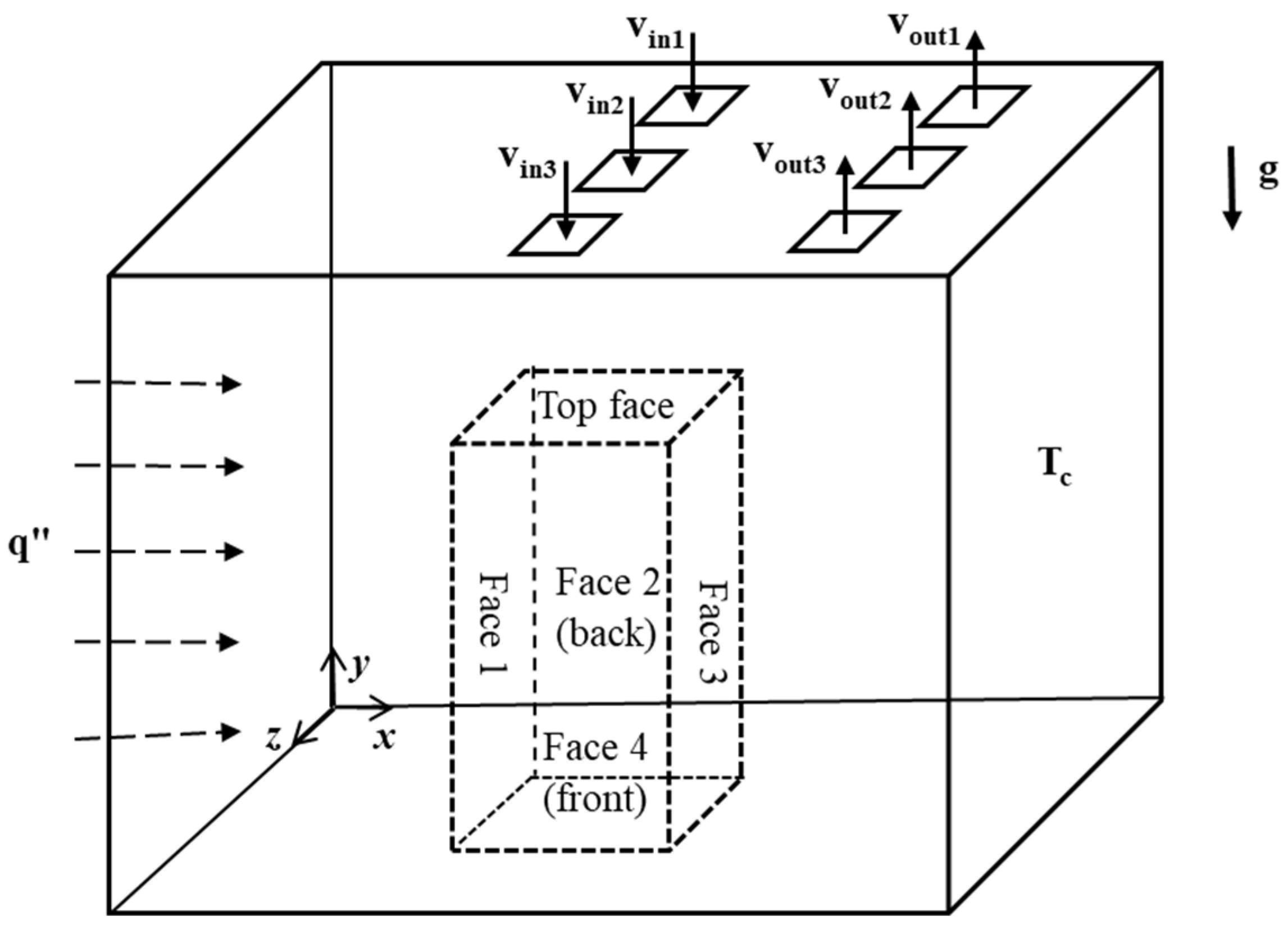
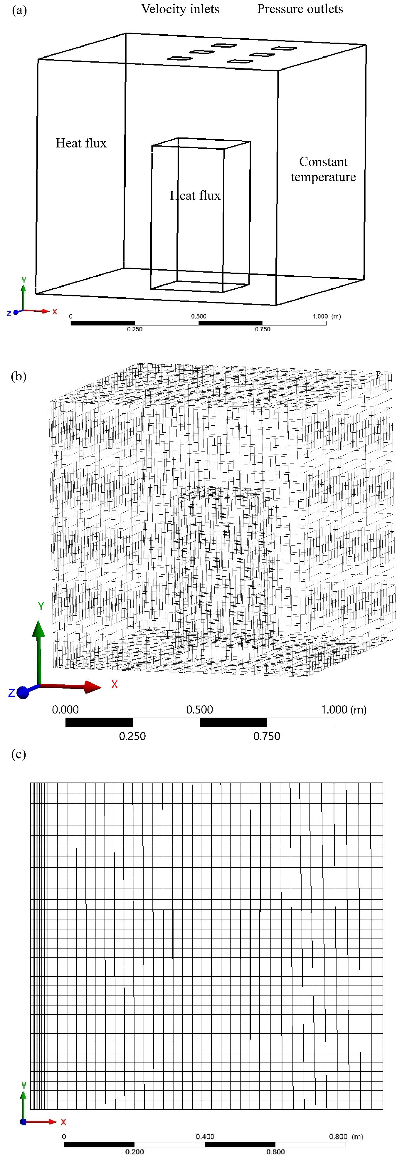
An analysis of turbulent convection was performed in a 1 m³ cavity (Lx = Ly = Lz = 1.0 m), as illustrated in Figure 1. The system consisted of a left vertical wall subjected to a constant uniform heat flux and an opposing vertical wall maintained at a constant temperature, Tc. All other walls were adiabatic. To minimize radiative heat exchange, every wall was lined with polished aluminum. The fluid in the cavity is air. A central parallelepiped (0.61 m height × 0.30 m depth × 0.30 m length), shown with dotted lines, housed electric resistances on all surfaces to simulate the heat generation of a human occupant. The presented cases are: 1. No thermal source: when there is no parallelepiped inside of the cavity, 2. Thermal source off: when the parallelepiped is located inside the cavity but is not generating heat, and 3. The thermal source in the parallelepiped at the interior is generating heat. The dimensions of the entrances and exits of air are 8 cm (all of them at y = 1 m) and the locations of the entrances are 0.46 m ≥ x ≤ 0.54 m at the x-coordinate, while the z-axis locations are 0.21 m ≥ z ≤ 0.29 m, 0.46 m ≥ z ≤ 0.54 m, and 0.71 m ≥ z ≤ 0.79 m, for inlets 1, 2 and 3, respectively. The outlets (located at 0.71 m ≥ x ≤ 0.79 m), the z-axis locations are 0.21 m ≥ z ≤ 0.29 m, 0.46 m ≥ z ≤ 0.54 m, and 0.71 m ≥ z ≤ 0.79 m for outlets 1, 2, and 3, respectively. The characteristic length for the Rayleigh number at the heated wall is the cavity’s edge dimension. The air at constant temperature enters the cavity with a velocity of 1.3 m/s. The fluid flow was assumed to be turbulent, with a Reynolds number of 7.7 × 10⁵.

2.2. Mathematical Model

The mathematical model is based on the following assumptions: steady-state conditions, air treated as Newtonian, flow in a turbulent regime, viscous dissipation negligible, and the Boussinesq approximation valid. The corresponding system of time-averaged governing equations in tensor notation is:

Continuity:

$${\displaystyle \frac{\mathsf{\partial }{\overline{u}}_i}{\mathsf{\partial }{x}_i}}=0$$

(1)

Momentum:

$$\rho {\overline{u}}_j{\displaystyle \frac{\mathsf{\partial }{\overline{u}}_i}{\mathsf{\partial }{x}_j}}={\displaystyle \frac{\mathsf{\partial }\overline{P}}{\mathsf{\partial }{x}_i}}+{\displaystyle \frac{\mathsf{\partial }}{\mathsf{\partial }{x}_j}}\left[\mu {\displaystyle \frac{\mathsf{\partial }{\overline{u}}_i}{\mathsf{\partial }{x}_j}}-\rho \overline{u_i^{\prime }{u}_j^{\prime }}\right]+\rho g_i\beta \left(\overline{T}-T_0\right)$$

(2)

Energy:

$$\rho {\overline{u}}_j{\displaystyle \frac{\mathsf{\partial }\overline{T}}{\mathsf{\partial }{x}_j}}={\displaystyle \frac{1}{C_p}}{\displaystyle \frac{\mathsf{\partial }}{\mathsf{\partial }{x}_j}}\left[\lambda {\displaystyle \frac{\mathsf{\partial }\overline{T}}{\mathsf{\partial }{x}_j}}-\rho C_p\overline{T^{\prime }{u}_j^{\prime }}\right]$$

(3)

where x_i and x_j are the Cartesian coordinates of the system (i = x, y, z and j = x, y, z), ū is the mean velocity, $\overline{P}$ is the mean dynamic pressure, $\overline{T}$ is the mean temperature, g is the gravitational acceleration; λ, ρ, C_p are the thermal conductivity, density, and the specific heat at constant pressure, respectively. The reference temperature (T₀) is the ambient temperature. However, the above set of equations is not complete due to the presence of the Reynolds stress tensor ($\rho \overline{u_i^{\prime }{u}_j^{\prime }}$) in the momentum equation and the turbulent heat flux vector ($\rho C_p\overline{T^{\prime }{u}_j^{\prime }}$) in the energy equation. To close the turbulence mathematical problem, a turbulence model must be considered.

This study evaluated six turbulence models: the standard k-ε (skε), realizable k-ε (rkε), RNG k-ε (rngkε), standard k-ω (skω), linear pressure-strain Reynolds stress model (rslps), and the Low-Re stress-omega model (rslrso). They are described briefly.

The standard k-ε model (skε) [33], a robust and economical semi-empirical model, remains popular for industrial applications due to its reasonable accuracy across a wide range of turbulent flows. It is a two-equation eddy viscosity model based on the Boussinesq hypothesis, which relates Reynolds stresses to mean velocity gradients and defines turbulent eddy viscosity as a function of turbulent kinetic energy (k) and its dissipation rate (ε). Several variants improve upon the standard model. The realizable k-ε model (rkε) [34] incorporates a new formulation for turbulent viscosity and a revised transport equation for the dissipation rate derived from an exact equation for vorticity fluctuations. The RNG k-ε model (rngkε) [35] includes refinements from renormalization group theory, such as an additional term in its ε equation for rapidly strained flows, built-in swirl effects, and an analytical formula for turbulent Prandtl numbers, unlike the user-defined constants in the skε model.

The standard k-ω model (skω) [36] is well-suited for wall-bounded and free shear flows (e.g., wakes, jets). It includes modifications for low-Reynolds-number effects and compressibility and accurately predicts shear-flow spreading rates. More complex Reynolds Stress Models (RSM) abandons the Boussinesq hypothesis. The low-Reynolds stress-omega model (rslrso) [36] is a stress-transport model based on the ω equation and is suitable for configurations involving curved and swirling surface flows. While it shares closure coefficients with the skω model, it includes additional ones to handle complex physics. The linear pressure-strain Reynolds stress model (rslps) [37] is the most complex RANS-based evaluated model. Instead of assuming isotropic viscosity, it resolves individual transport equations for each Reynolds stress component and an equation for ε, resulting in five additional equations to solve at two-dimensional problems, increasing to seven in three-dimensional situations.

2.3. Non-Dimensional Numbers Used

To generalize results, the nondimensional Reynolds and Rayleigh numbers were determined as:

$$Re={\displaystyle \frac{U_{in}{L}_y}{v}}$$

(4)

$$Ra={\displaystyle \frac{g\beta q^{″}{L}^4}{v\alpha \lambda }}$$

(5)

where ν is the kinematic viscosity, $q^{″}$ is the heat flux on the heated wall, α is the thermal diffusivity, L_y is the height of the cavity, U_in is the air inlet velocity, and λ is the thermal conductivity of the fluid.

The Nusselt number is defined as the ratio between the heat flux at the hot wall in the presence of natural convection and the heat flux due to conduction only, i.e.,

$$Nu={\displaystyle \frac{q_{convective}}{q_{conductive}}}={\displaystyle \frac{hL}{\lambda }}$$

(6)

where h is the convective heat transfer coefficient.

3. Experimental System

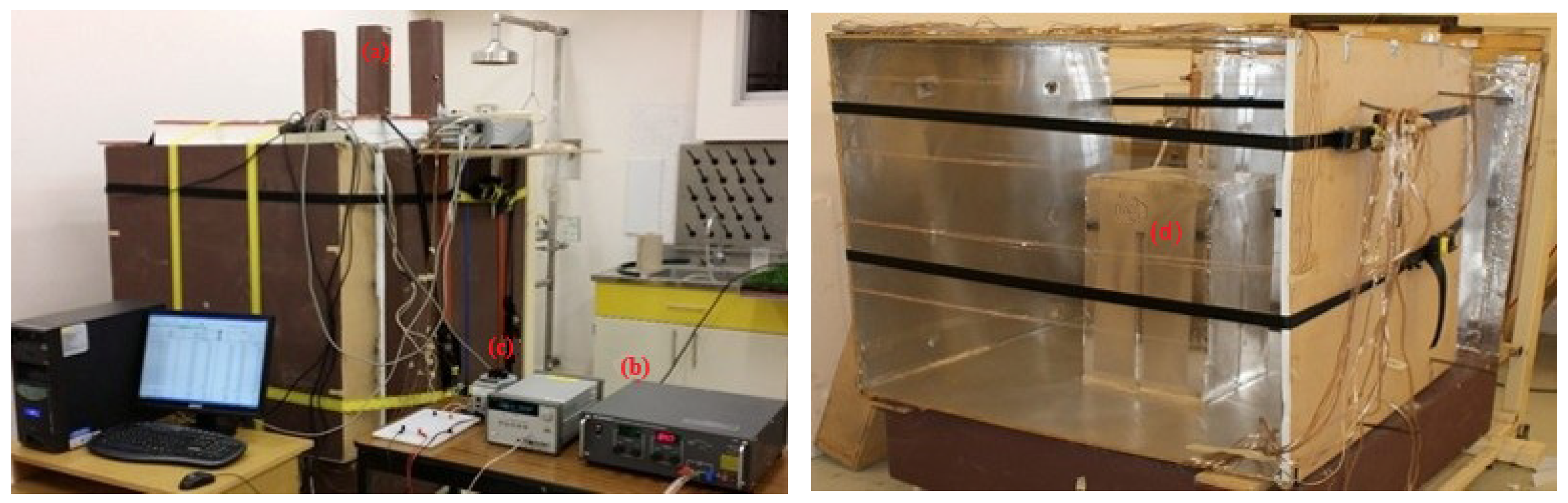
The experimental cavity is shown in Figure 2. The walls of the cavity were built of medium-density fiberboard (MDF) with a 0.05 m-thick polystyrene core. The hot wall has an electrical heater covered with silicon, measuring 0.91 m × 1.01 m. The electrical heater is in contact with an aluminum plate to better distribute heat across the hot face of the cavity wall, and it is supported in a box of medium-density fiberboard (MDF) with 0.1 m of mineral wool and 0.1 m of polystyrene as thermal insulation. The electrical heater is connected to a Powerstat AC variable autotransformer model 3PN136B, allowing the electrical tension to be adjusted to obtain the desired thermal power. To keep the right wall of the cavity isothermal, a heat exchanger from the TEMP-PLATE brand is connected to the Cole-Parmer thermostatic bath, using water as the thermal fluid. The internal heat source is a parallelepiped (base dimensions of 0.3048 m × 0.3048 m and a height of 0.6096 m) filled with mineral wool. The walls are made of MDF and are covered with Omega-brand electrical heaters. Three thermocouples are placed at each vertical surface and one at the top surface. The electrical heaters in the vertical surfaces are connected in parallel to a high-current DC regulating power supply, and the top surface to a single-output programmable DC power supply. All the surfaces inside the cavity are covered with polished aluminum sheets (ε_r ≈ 0.03).

The data acquisition system is composed of three Agilent data acquisition system model 34970A, with three multiplexor cards and a capacity of 20 thermocouples each. To monitor the temperature inside the cavity, 84 k-type calibrated thermocouples with a diameter of 0.079 mm (40 AWG) are used, with a calculated uncertainty of ±0.8 °C. The thermocouples formed an array of six temperature profiles at the following heights: y = 0.25 m, 0.50 m, 0.75 m, and 0.9 m, and at the following depths: z = 0.25 m, 0.50 m, and 0.75 m. At every temperature profile, 14 thermocouples are placed at the following positions on the x-axis: 0 m, 0.004 m, 0.008 m, 0.012 m, 0.016 m, 0.02 m, 0.03 m, 0.97 m, 0.98 m, 0.984 m, 0.988 m, 0.992 m, 0.996 m, and 1.0 m. Additionally, 12 thermocouples are located on an aluminum film attached to the hot surface to measure heat losses. There were no thermocouples in the middle of the cavity due to the location of the internal heat source, as shown in Figure 2b. Three thermocouples measure the air temperature at the outlets, and one thermocouple monitors the milieu temperature.

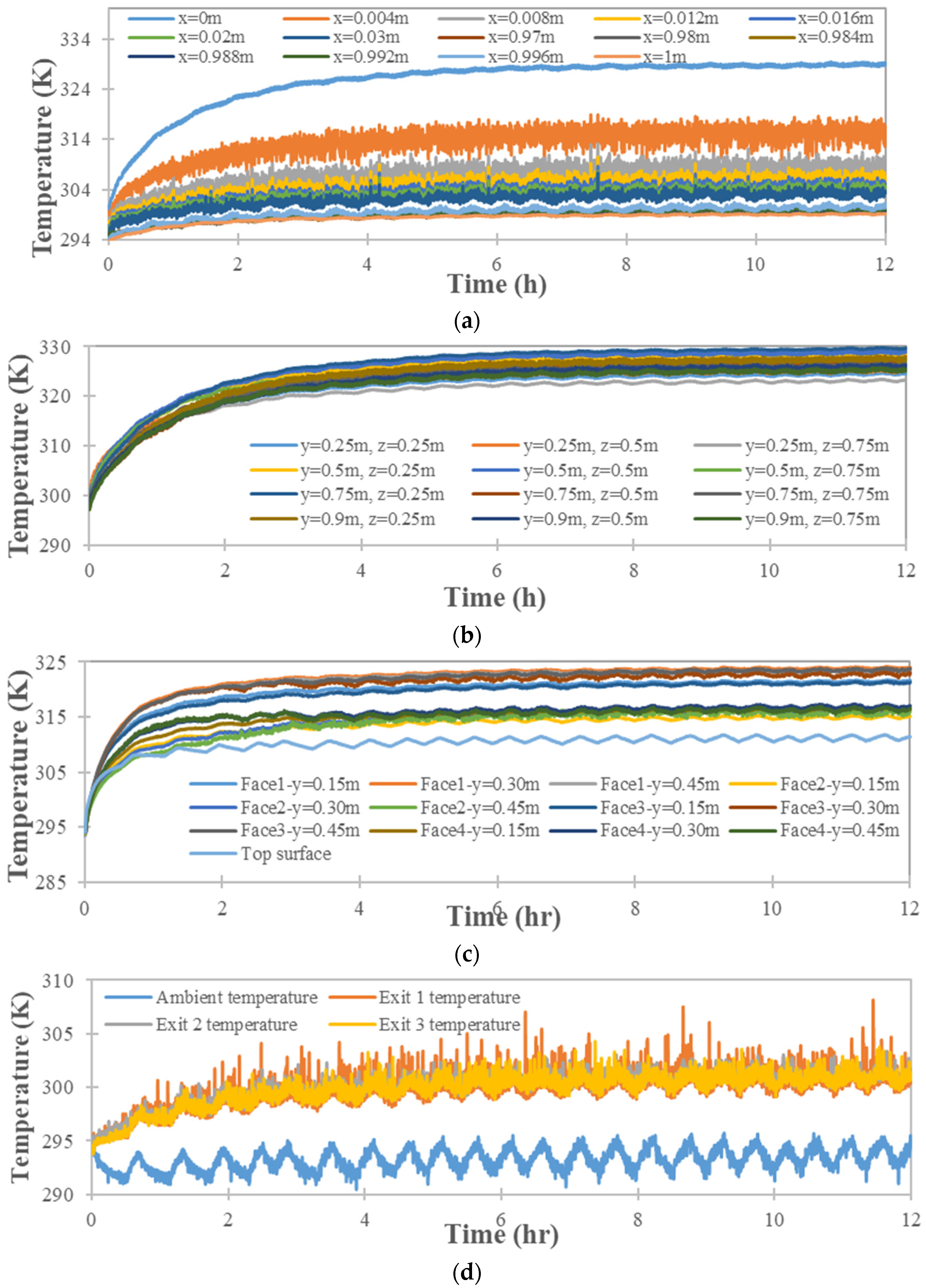
The experiment initiates by setting the heat power to the hot wall (and the heat source) and adjusting the desired air velocity at the inlets. The monitoring interval for temperature data was 10 s, for a total of 12 h. The temperature data processing is illustrated in Figure 3 with the results obtained for a Rayleigh number of 5.5 × 10¹¹ (computed with the heat power applied to the heated wall). The experimental data is plotted from the beginning to the end of the experiment. The temperatures of the heated wall, the ambient temperature, the air outlets, and the air inside the cavity are analyzed. In Figure 3a, it can be observed that, at every position in the cavity, the temperature varies with time, indicating the presence of a turbulent flow regime.

To compare experimental and numerical results (since the turbulence models are based on the Reynolds Averaged Navier-Stokes Equations), the experimental values are time-averaged. The heated wall temperature indicates that after five to six hours, it reaches its maximum value and remains practically constant throughout the experiment. In Figure 3b–d, the effect of the time-average treatment (interval of 3 h) on the temperatures of the air inside the cavity, incoming air, and heated wall, respectively, is shown.

Newton’s law computes the experimental values of the convective coefficient (h):

$$q^{″}=hA\left({\overline{T}}_h-{\overline{T}}_c\right)$$

(7)

Considering $q^{″}$ = VI, hence:

$$h={\displaystyle \frac{VI}{A\left({\overline{T}}_h-{\overline{T}}_c\right)}}$$

(8)

where V is the electric tension and I is the current applied to the electrical heater.

4. Numerical Procedure

The computational fluid dynamics study was performed using Ansys Fluent 18 software that solves the governing fluid motion equations using the finite volume method. The pressure-velocity coupling was resolved using the SIMPLE algorithm, while the convective terms were discretized using the MUSCL scheme [38]. A solution was considered converged when the normalized residuals fell below 1 × 10⁻⁶ for all variable balances. The physical model of Figure 1, created with design modeler software and a surface plane at z = 0.5 m, is shown in Figure 4a,b. The conformal hexahedral element mesh has a bias toward the hot wall (left wall) to capture the thermal boundary layer phenomena.

The thermal boundary conditions consisted of a uniform, constant heat flux on the hot wall and the internal heat source, a constant temperature on the cold wall, and adiabatic conditions on the remaining walls. Non-slip conditions were applied at all walls, setting all velocity components to zero. At the inlet, air entered perpendicularly; thus, a constant velocity was specified for the normal component (y-direction), while the tangential components were fixed to null. The fluid thermophysical properties were assumed to be constant at 300 K as can be seen at

Table 1. Fluid thermophysical properties [39].

Cp, (J/(kg·K))	1007
β, (1/K)	0.0033
ν, (m2/s)	15.89 × 10−6
λ, (W/(m·K))	26.3 × 10−3
μ, (N·s/m2)	184.6 × 10−7
ρ, (kg/m3)	1.1614

.

A pressure-outlet boundary condition was applied to the leaving flow. Inflow values for turbulent kinetic energy and its dissipation rate were prescribed using established empirical correlations [40].

$$k_{in}=1.5{\left(0.04U_{in}\right)}^2$$

(9)

$${\mathsf{\epsilon }}_{t,in}={\displaystyle \frac{{\left(k_{in}\right)}^{1.5}}{l_y}}$$

(10)

A grid independence study was performed to determine an appropriate mesh size, fixing the y and z axes at 30 nodes and varying the number of nodes in the x-coordinate, since this is the direction of the thermal gradient. This study was conducted with the internal heat source activated under the following conditions: a total heat flow of 150 W applied to the hot wall, a heat generation rate of 128 W from the thermal source, and an air inlet velocity of 1.3 m/s at the system inlets. The average Nusselt number at the hot wall for the different mesh configurations is shown in

Table 2. Independence mesh study with 30 nodes fixed on the y and z axes.

x-Axis Nodes	Nusselt Number of the Heated Wall	$\mathbf{D}\mathbf{i}\mathbf{f}\mathbf{e}\mathbf{r}\mathbf{r}\mathbf{e}\mathbf{n}\mathbf{c}\mathbf{e}$ (%)
20	147	---
30	149	1.1
40	148	0.1
50	149	0.5

, where it can be observed that the variations become negligible (less than 1%) when a discretization of 30 nodes in the x-direction is reached, resulting in a mesh with 27,000 elements.

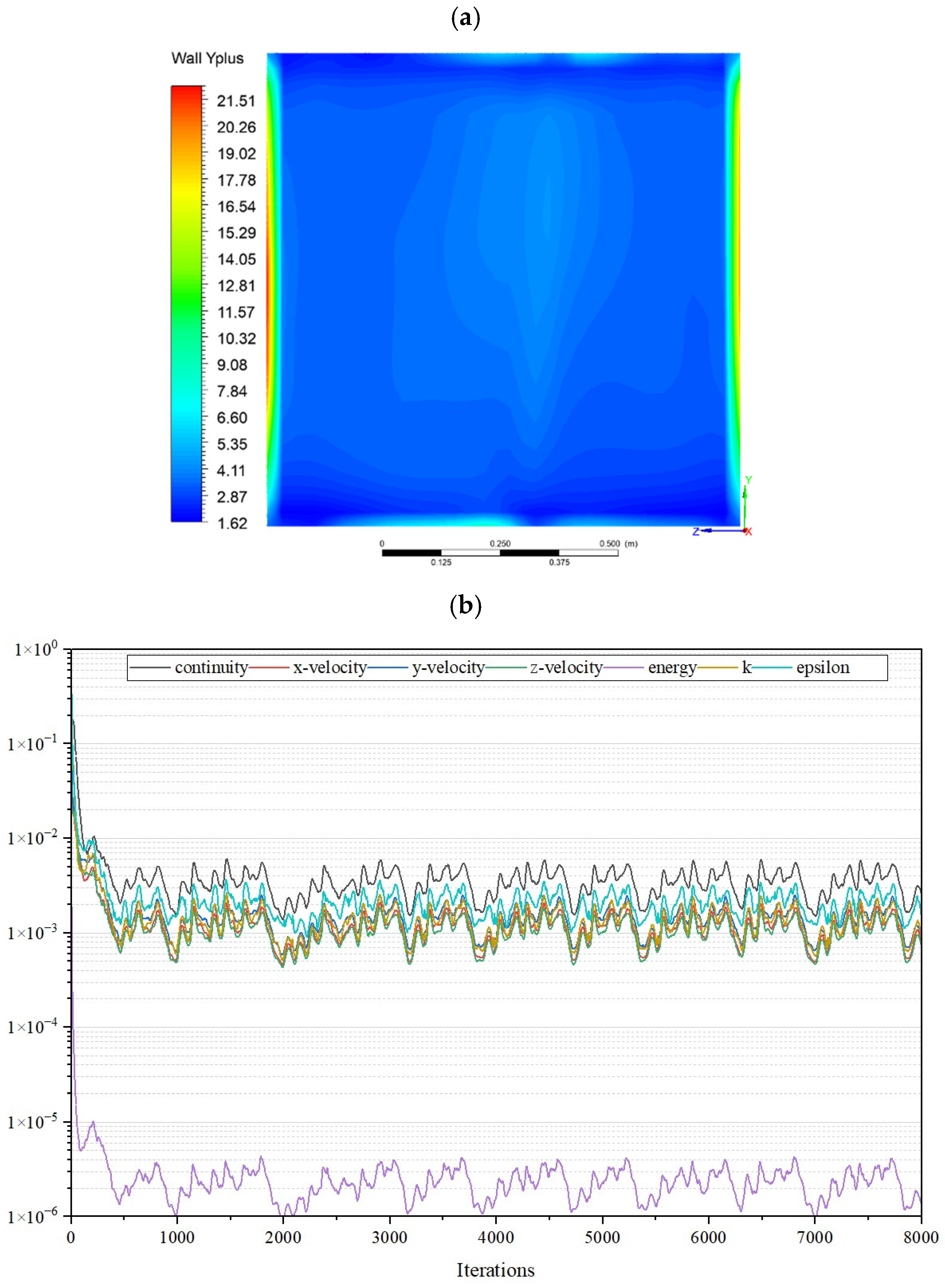
The system mesh orthogonal quality yielded values very close to 1, with the lowest-quality element at 0.98, indicating excellent alignment between grid elements and contributing to improved numerical stability. The y+ values on the hot wall are shown in Figure 5a, where a very uniform distribution with an average of 3.32 is observed. However, localized increases in y+ were identified near the lateral edges of the wall. Their impact is not considered significant, as these regions are adjacent to adiabatic surfaces and far from the region where most heat transfer occurs. According to the Law of the Wall, the linear viscous sublayer is located at y+ < 5; therefore, it is concluded that the boundary layer is properly resolved. The residuals evolution for the thermal source on case is presented in Figure 5b where it can be observed the steady values from the 1000 iterations onwards. This is similar for the no thermal source and thermal source off cases.

5. Results Analysis

The results correspond to a heated wall Rayleigh number of 5.5 × 10¹¹ (150 W), a Ra = 4.6 × 10¹¹ in the thermal source (128 W), and a Re = 7.7 × 10⁵ (corresponding to a velocity value of 1.3 m/s). The experimental uncertainty was obtained according to [41].

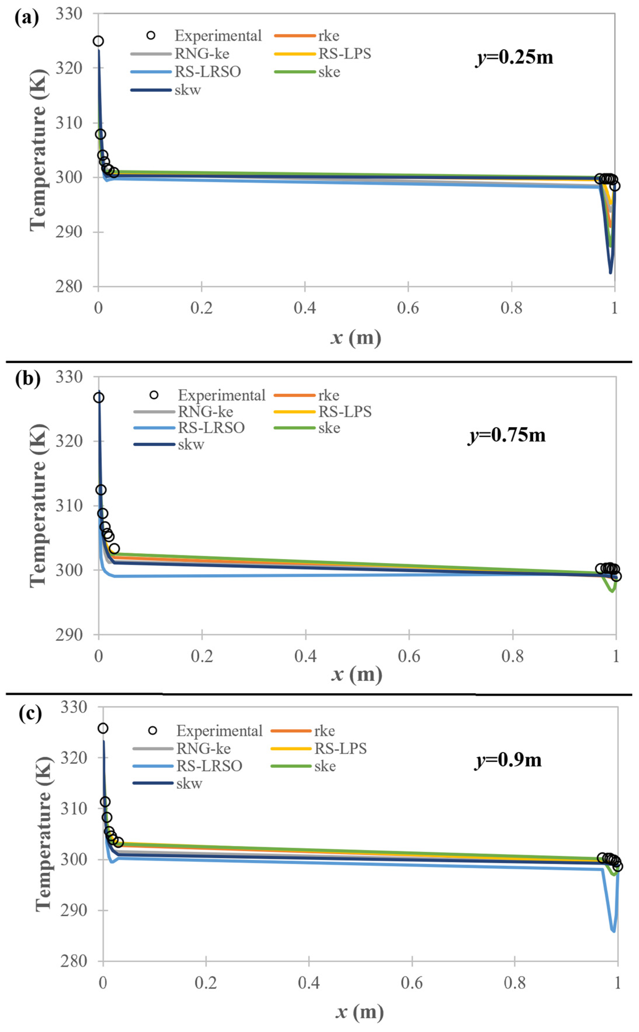
Figure 6 shows the numerical temperature profiles at z = 0.5 m, along with the experimental data, when the heat source is on. Also, at y = 0.25 m, a 325 K temperature is observed at the hot wall. The trend is downward along the x-axis, and there is an underprediction of the lower-temperature wall boundary layer. For y = 0.75 m, the maximum temperature at the hot wall is 326 K, and there is an under-prediction in both boundary layers adjacent to the hot and cold walls. For y = 0.9 m, the highest experimental temperature value is 325 K at the hot wall, and the behavior of all the turbulence models is the same: they underpredict the temperatures. It can be observed that the rslrso model shows greater deviation in the lower-temperature wall boundary layer.

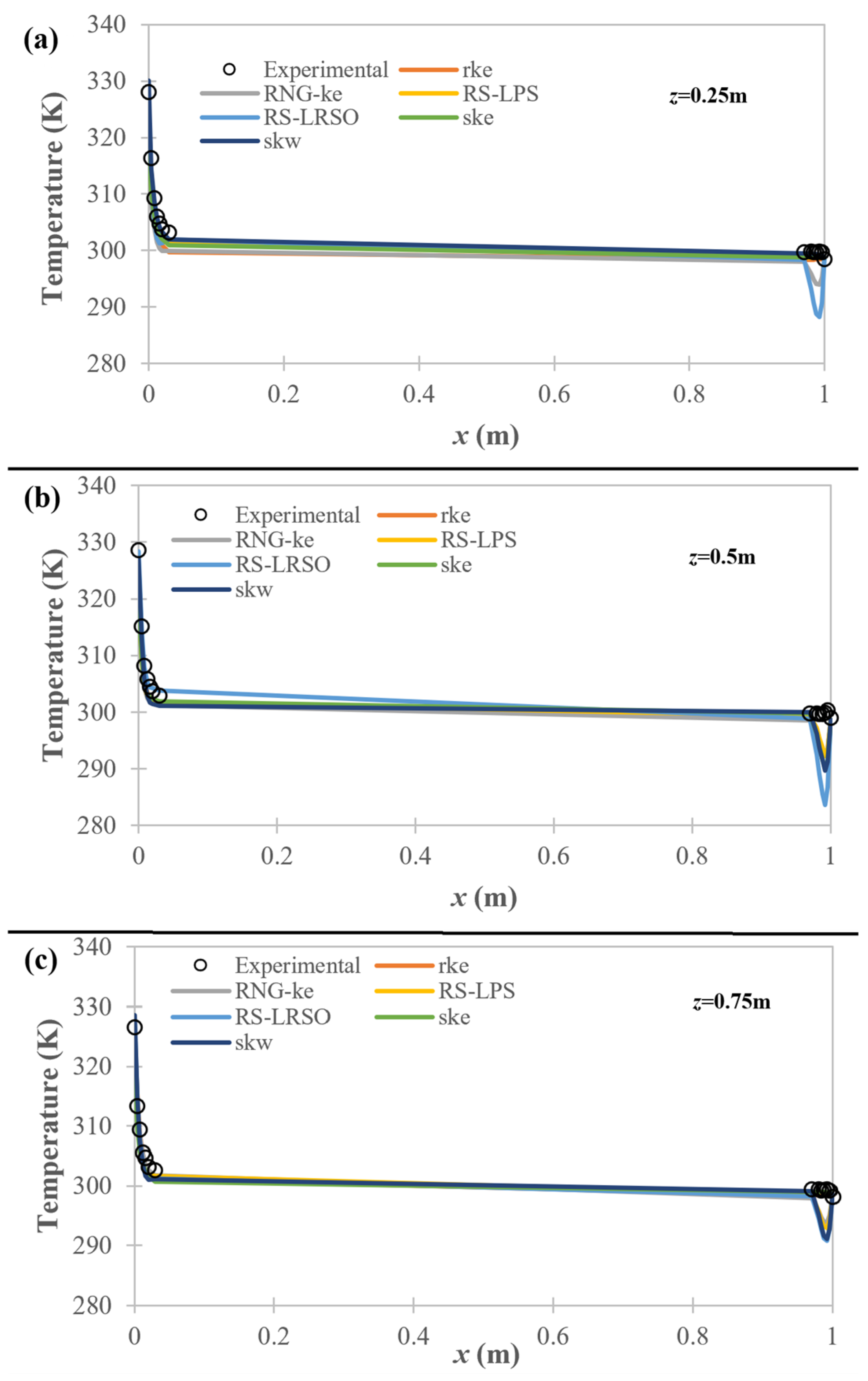
In Figure 7, the experimental and numerical temperature profiles for the thermal source case at y = 0.5 m are shown. In the z = 0.25 m position, a maximum value of 328 K (at x = 0 m). For z = 0.5 m, the temperature at the hot wall is 328 K. Finally, at z = 0.75 m, the temperature at the heated wall is 326 K. In the three cases, an underprediction of the numerical results at the boundary layer of the cold wall is observed, and the middle profile (z = 0.5 m) shows the largest difference.

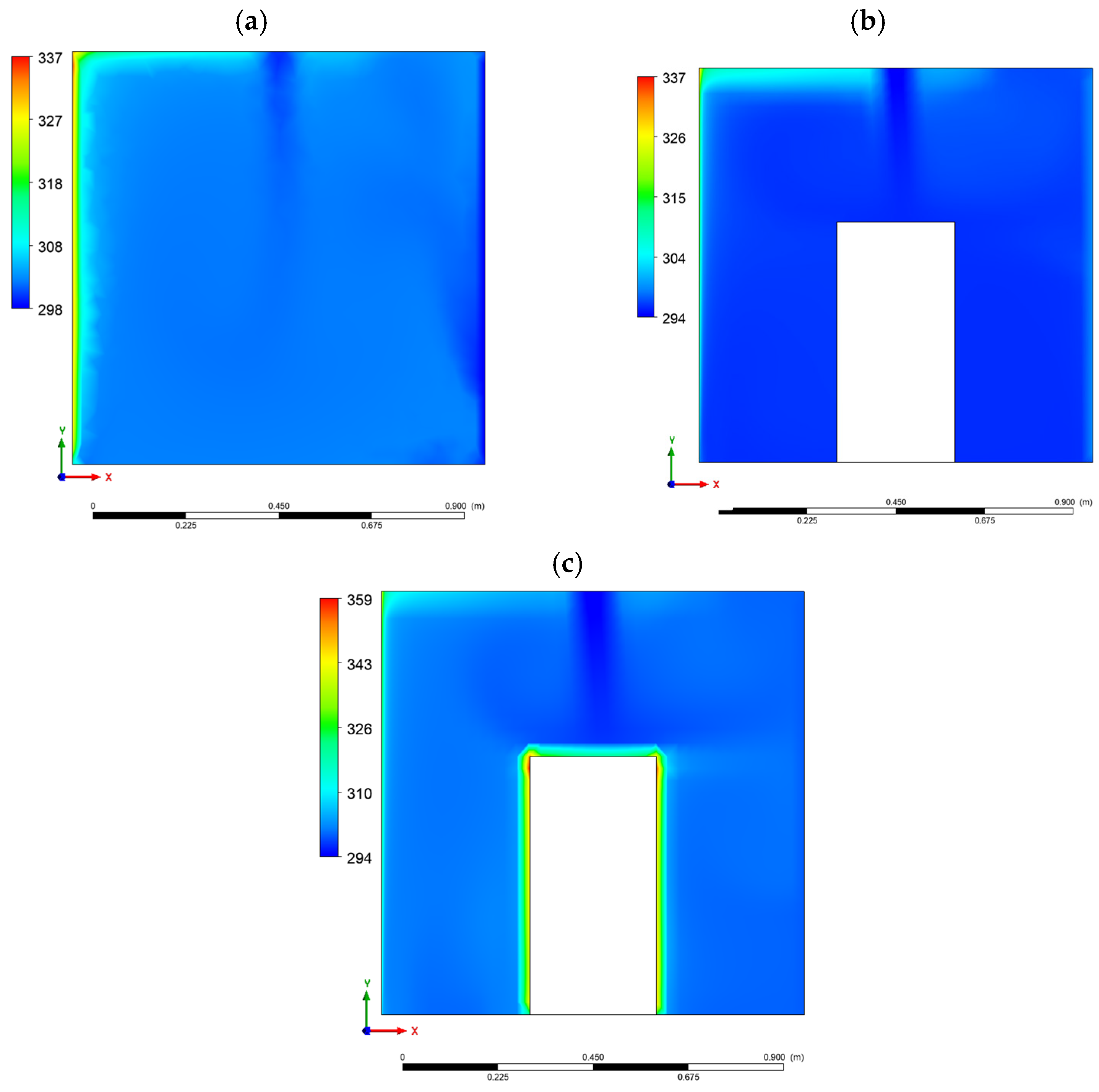
The temperature contours presented at Figure 8, exhibit that for the cavity without heat source (Figure 8a) most of the plane present a 305 K temperature value, but near the cold wall where it can be appreciated a 300 K value; the hot wall presents a thermal boundary layer with a thickness near to 0.05 m, but this value increases till 0.07 m at 0.9 m height where the fluid reaches the top surface and begins to exit the cavity. This behavior is interrupted because the inlet port at 0.5 m along the x-axis has a 300 K temperature, yet appears as a zone with a 310 K temperature. In the thermal source off case (Figure 8b), most of the cavity has a 300 K temperature, and the thermal boundary layer is thicker than in the case without a heat source. In the environs of the cold wall, a thermal boundary layer cannot be observed. Finally, for the case with the heat source on (Figure 8c), the contour presents regions with a temperature value of 300 K; the thermal boundary layer at the hot wall reduces its thickness compared with the prior cases, and the heat source presents a thermal boundary layer of about 0.025 m thickness at all of its surfaces. The maximum temperature for the case without a heat source is 335 K, and for the case with a heat source, it is 355 K.

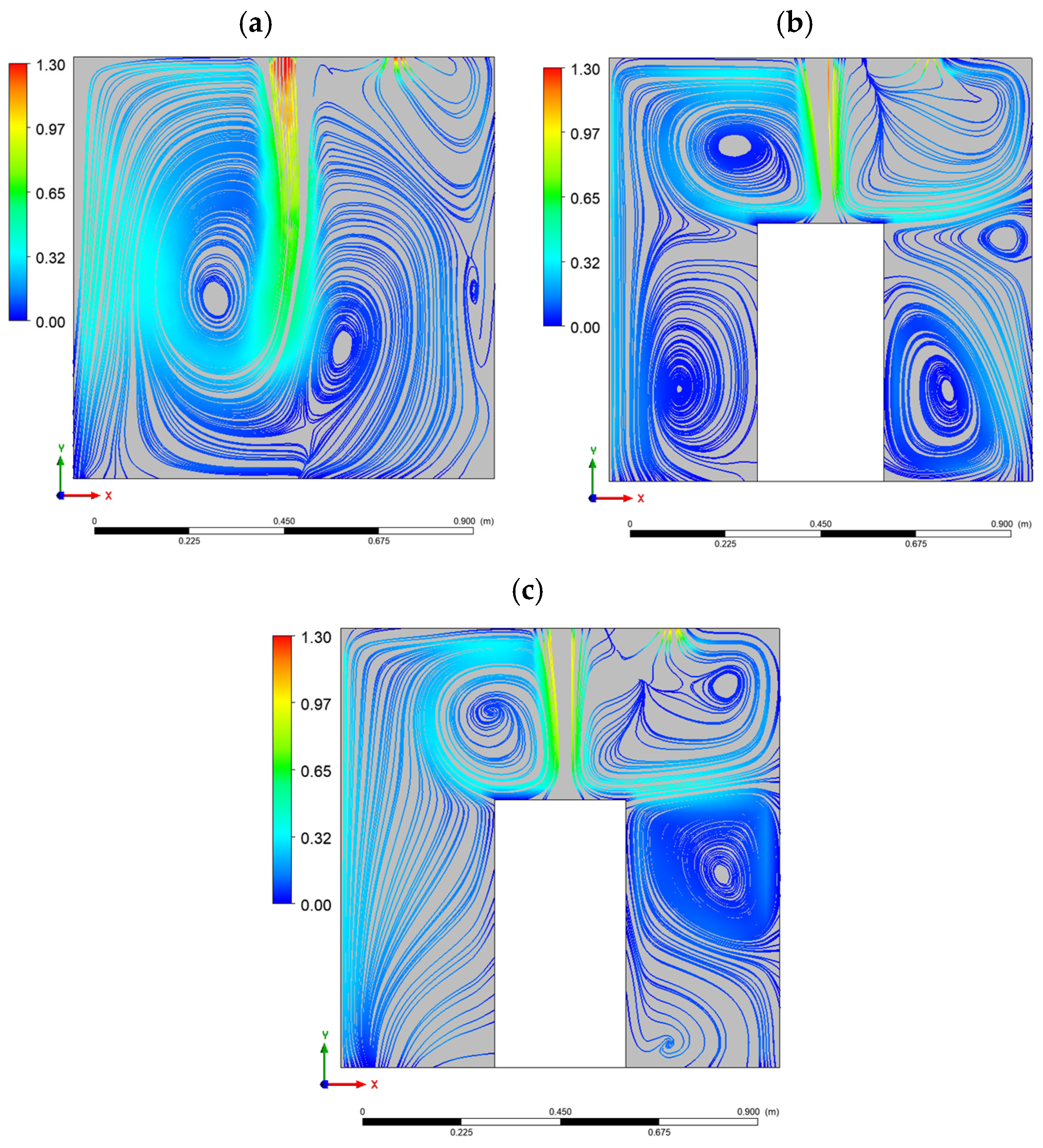
The velocity streamlines at the plane z = 0.5 m in Figure 9 indicate that, for the case without a heat source (Figure 9a), the fluid enters through the middle of the cavity and, when it nearly reaches the bottom surface, it deflects its course at a height of 0.20 m from the floor. The fluid ascends through the hot wall, reaches the top surface, and begins its way to the cavity exit when it is interrupted by the impinging jet. On the other hand, the behavior on the cold wall is irregular, with no defined path. Also, a major vortex can be seen in the middle-left part of the plane, and a minor one on the lower right side. In the thermal source off case (Figure 9b), fluid enters the cavity and reaches the parallelepiped, deflecting its course and forming a clockwise vortex at the upper left of the plane. The fluid ascends along the heated wall until it is interrupted by the top surface, then flows over to the exit. On the cold wall side, the fluid descends to the lower half and recirculates, whereas on the upper half, it rapidly ascends to the cavity exit. Finally, for the case with the thermal source on (Figure 9c), the fluid exhibits a similar behavior to the heat source case, but the heat source’s input of energy defines the fluid path, especially in the vicinity of the cold wall.

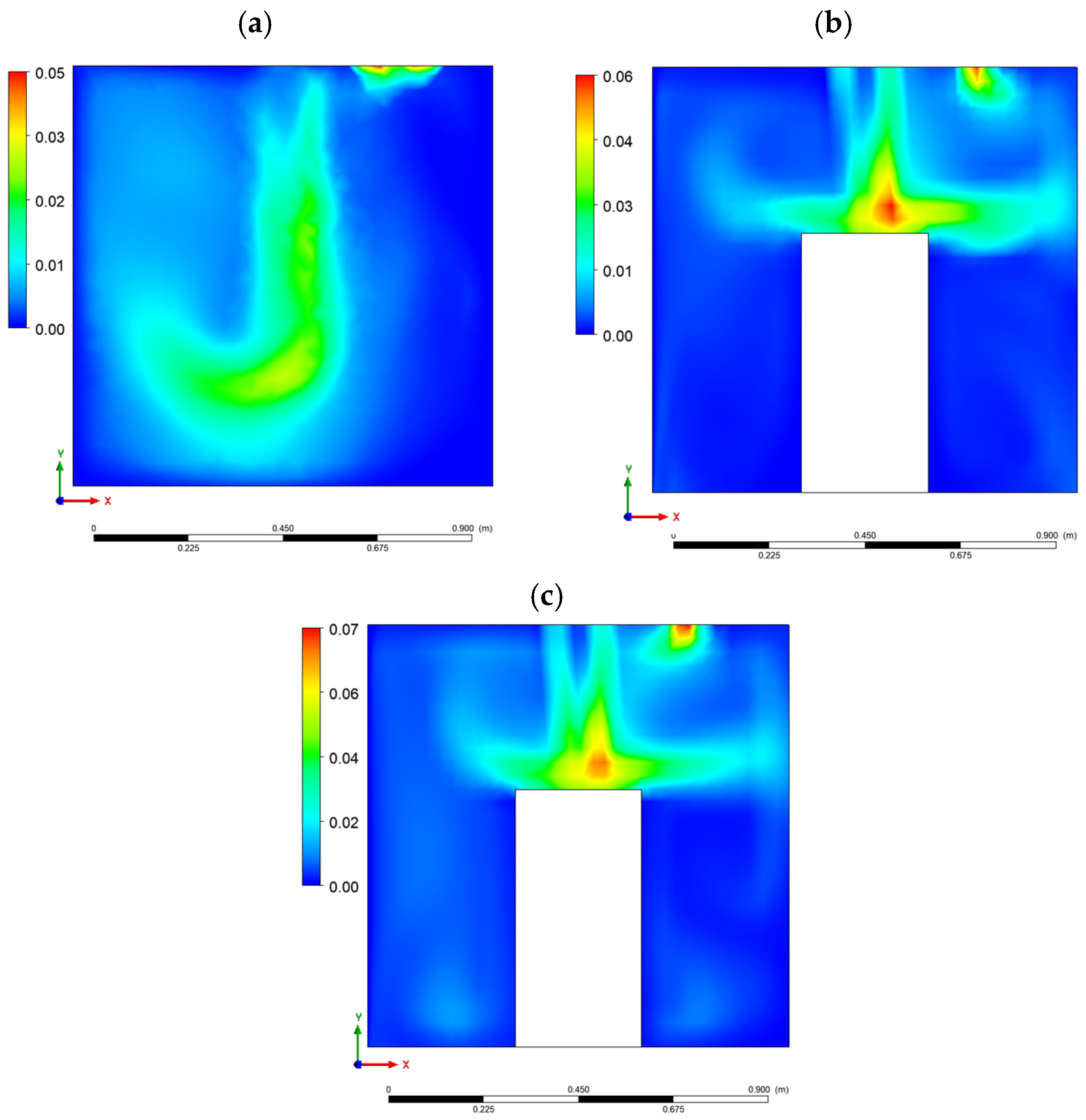
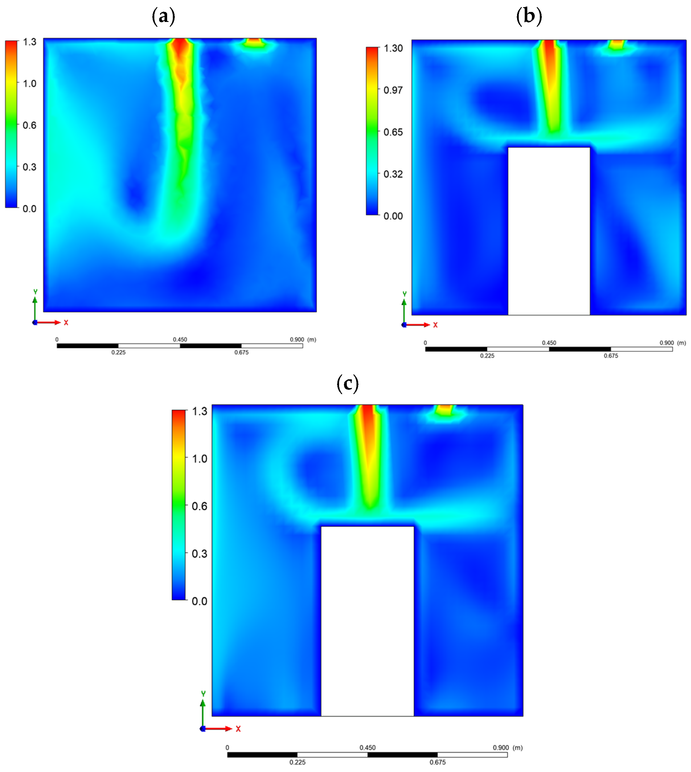
Figure 10 presents the velocity magnitude contours (m/s) at the plane z = 0.5 m. It shows that, in the case with no heat source (Figure 9a), most of the fluid at the plane has a velocity of 0.2 m/s. At the inlet, the fluid velocity passes from the fixed value of 1.3 m/s to a 0.4 m/s value. Near the hot wall, a portion of the fluid reaches a velocity of 0.6 m/s, and at the cavity exit, the fluid leaves with a velocity of 1.2 m/s. On the other hand, the case with the heat source off (Figure 10b) exhibits zones with about 0.1 m/s around the bottom, the source, and the cold wall. However, the velocity magnitude increases to 0.4 m/s at the hot wall, and a zone with values between 0.5 and 1.2 m/s is observed over the source produced by the incoming air. The zone where the fluid goes out has velocities between 0.6 and 1.2 m/s. Finally, the case with the heat source on (Figure 10c) displays zones with a value of 0.1 m/s, around the source and the proximity of the cold wall; at the hot wall the velocity of the fluid rises to 0.4 m/s, at the inlet zone it goes from the fixed value till a 0.6 m/s velocity magnitude; and at the exit zone the velocity magnitude goes from 0.6 to 1.2 m/s.

The turbulent kinetic energy contour at plane z = 0.5 m is shown in Figure 11. The case with no internal heat generation (Figure 11a) indicates a 0.005 m²/s² value for most of the planes, but in the center, a zone with a maximum value of around 0.03–0.035 m²/s², and finally, at the exit zone, the value increases to 0.045 m²/s². On the other hand, the heat source off case (Figure 11b) shows a zone at the top surface of the source with values above 0.045 m²/s², and the distribution decreases to 0.005 m²/s² at the source and the hot vertical walls. Finally, for the heat source in case (Figure 11c), the minimum values are distributed at the hot wall, the vertical walls of the source, and the cold wall, with a value of 0.005 m²/s². The maximum value at the plane is on the upper surface of the source, where it ranges from 0.004 to 0.025 m²/s².

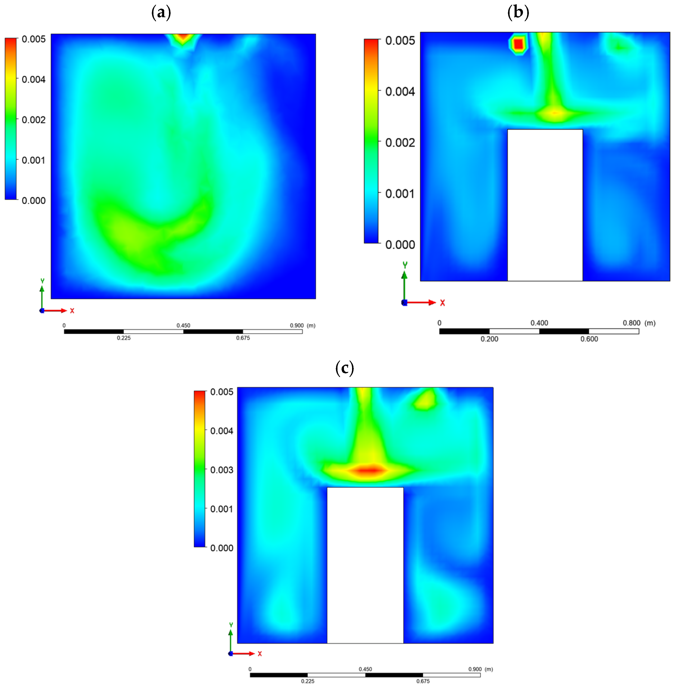
Figure 12 presents the turbulent viscosity contours for the three cases. For the no internal heat generation case (Figure 12a), the minimum is near the cavity walls, with a value of 5 × 10⁻³, while the maximum is at the inlet, with values above 4 × 10⁻³. At the center of the plane, a considerable area is observed with values between 1.5 × 10⁻³ and 3.5 × 10⁻³ kg/m-s. For the case with the heat source off (Figure 12b), at the superior area of the plane, at the inlet and outlet, the value of turbulent viscosity goes above 0.004 kg/m-s, whilst in the zones at the proximity of the cavity and source walls, this value decreases to 0.0005 kg/m-s. Finally, for the case with the heat source on (Figure 12c), the maximum value of 1.5 × 10⁻³ is in the zones next to the source, while the rest of the plane presents values between 0.001 and 0.005 kg/m-s.

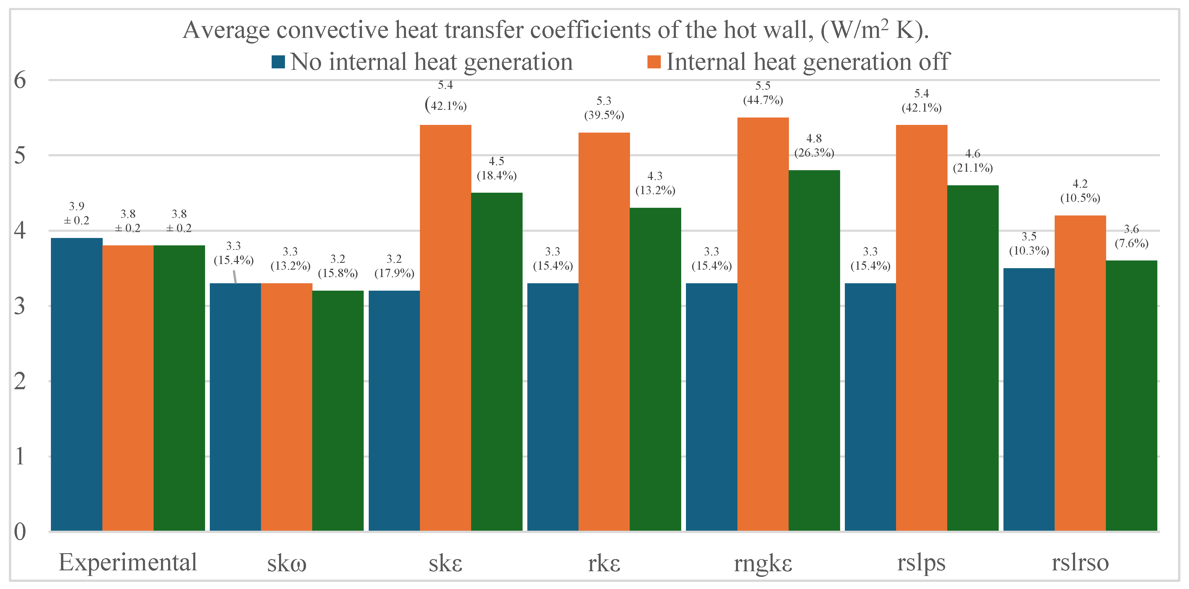
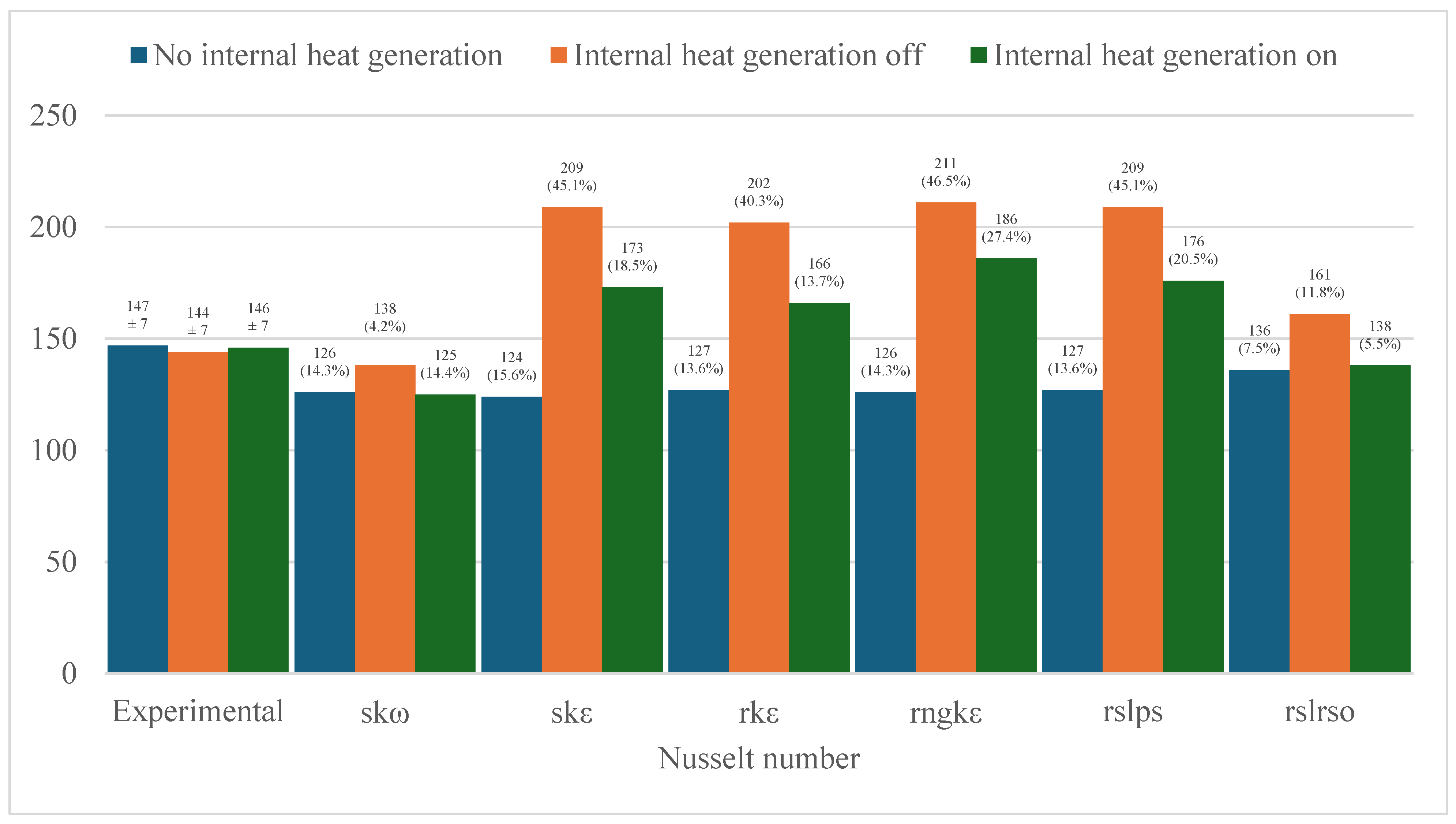
A comparison of the experimental and numerical results for the average convective heat transfer coefficient and the Nusselt number of the heated wall is presented in Figure 13 and Figure 14, respectively.

The agreement between the models and experiment varied significantly. For the average convective heat transfer coefficient of Figure 12, in the case of no internal heat generation, the turbulence model rslrso performed best (with a difference of 7.6%), and the k-ε standard turbulence model showed the largest discrepancy (17.9% difference). When the thermal source was present but turned off, the rslrso model was most accurate (10.5% difference), and the RNG k-ε model was least accurate (~45% difference). At the thermal source on the case, the rslrso model again provided the best agreement (7.6% difference), whereas the RNG k-ε model yielded the largest error (26.3% difference). Whilst for the Nusselt number, this remains with better and worse approximations for the rslrso and ske turbulence models, with 5.5% and 13.6%, respectively, for the no internal heat generation case. When the source is placed inside the cavity but remains off, the standard k-ω turbulence model exhibits the lowest difference of 4.2% and with the RNG k-ε model the highest difference of 46.5%. Finally, when the heat source is turned on, the rslrso and the RNG k-ε model have the best and worst approximations, with 5.5% and 27.4%, respectively.

Critically, the experimental values themselves were largely unaffected by the state of the internal heat source. The average convective heat transfer coefficient remained nearly constant, ranging from 3.8 to 3.9 W/(m²·K) with a calculated uncertainty of ±0.2, and the Nusselt number oscillated only between 144 and 147 with an uncertainty of ±7. It indicates that the presence of the heat source (whether on or off) has a negligible influence on the heat transfer dynamics of the heated wall.

The comparison between experimental and numerical temperature profiles at the cross-sections y = 0.5 m and z = 0.5 m (

Table 3. Temperature profiles at y = 0.5 m, z = 0.5 m for the no thermal source case, (K).

x (m)	Exp.	rkε	$\mathit{\Delta }$, %	rngkε	$\mathit{\Delta }$, %	skε	$\mathit{\Delta }$, %	rslrso	$\mathit{\Delta }$, %	rslps	$\mathit{\Delta }$, %	skω	$\mathit{\Delta }$, %
0	326.4 ± 0.3	306.0	6.2	329.3	0.9	326.3	0.0	321.5	1.5	327.3	0.3	309.3	5.2
0.004	310.6 ± 1.8	304.4	2.0	303.7	2.2	317.3	2.2	314.0	1.1	317.7	2.3	306.6	1.3
0.008	303.9 ± 1.3	303.3	0.2	303.3	0.2	311.4	2.4	309.0	1.7	311.3	2.4	304.8	0.3
0.012	301.2 ± 1.1	302.6	0.5	303.2	0.7	307.6	2.1	305.8	1.5	307.2	2.0	303.7	0.8
0.016	299.9 ± 0.9	302.1	0.7	303.3	1.1	305.2	1.8	303.9	1.3	304.7	1.6	303.0	1.0
0.02	299.4 ± 0.9	301.9	0.8	303.3	1.3	303.9	1.5	302.8	1.1	303.3	1.3	302.6	1.1
0.03	298.7 ± 0.9	301.7	1.0	303.1	1.5	302.7	1.3	301.9	1.1	302.0	1.1	302.3	1.2
0.97	297.6 ± 0.7	301.4	1.2	300.4	0.9	300.9	1.1	301.3	1.2	299.8	0.7	302.1	1.5
0.98	297.6 ± 0.7	301.1	1.2	300.0	0.8	300.4	0.9	300.9	1.1	299.5	0.6	301.8	1.4
0.984	297.8 ± 0.7	300.9	1.1	299.8	0.7	300.1	0.8	300.6	0.9	299.3	0.5	301.5	1.3
0.988	297.9 ± 0.7	300.5	0.9	299.5	0.5	299.6	0.6	300.2	0.8	299.0	0.4	301.1	1.1
0.992	298.0 ± 0.6	300.0	0.7	299.1	0.4	299.1	0.4	299.6	0.5	298.7	0.2	300.4	0.8
0.996	298.5 ± 0.6	299.1	0.2	298.6	0.0	298.5	0.0	298.9	0.1	298.3	0.0	299.3	0.3
1	298.2 ± 0.1	297.9	0.1	297.9	0.1	297.9	0.1	297.9	0.1	297.8	0.1	297.9	0.1

,

Table 4. Temperature profiles at y = 0.5 m, z = 0.5 m for the thermal source off case, (K).

x (m)	Exp.	rkε	$\mathit{\Delta }$, %	rngkε	$\mathit{\Delta }$, %	skε	$\mathit{\Delta }$, %	rslrso	$\mathit{\Delta }$, %	rslps	$\mathit{\Delta }$, %	skω	$\mathit{\Delta }$, %
0	327.0 ± 0.4	321.3	1.8	317.9	2.8	317.0	3.1	325.6	0.4	316.9	3.1	327.0	0.0
0.004	312.7 ± 1.5	310.6	0.6	309.4	1.0	307.0	1.8	312.1	0.2	307.2	1.7	312.6	0.0
0.008	304.5 ± 1.2	304.4	0.0	304.1	0.1	302.2	0.7	304.9	0.1	302.1	0.8	304.8	0.1
0.012	301.4 ± 1.0	301.0	0.1	300.9	0.2	299.9	0.5	301.8	0.1	299.6	0.6	301.4	0.0
0.016	299.8 ± 0.8	299.1	0.2	299.0	0.3	298.6	0.4	300.2	0.1	298.6	0.4	299.8	0.0
0.02	299.0 ± 0.7	298.2	0.3	298.0	0.3	298.0	0.4	299.2	0.1	298.2	0.3	299.0	0.0
0.03	298.1 ± 0.7	297.5	0.2	297.2	0.3	297.1	0.3	298.0	0.0	297.9	0.1	298.1	0.0
0.97	295.6 ± 0.6	295.4	0.1	295.6	0.0	295.6	0.0	295.7	0.1	295.0	0.2	296.3	0.2
0.98	295.6 ± 0.6	292.8	0.9	296.4	0.3	295.6	0.0	295.8	0.1	290.3	1.8	296.3	0.3
0.984	295.6 ± 0.6	291.5	1.4	296.8	0.4	295.6	0.0	295.9	0.1	287.9	2.6	296.3	0.3
0.988	295.6 ± 0.6	290.5	1.7	297.2	0.5	295.7	0.0	295.9	0.1	286.0	3.3	296.4	0.3
0.992	295.8 ± 0.6	290.1	1.9	297.4	0.5	295.8	0.0	296.1	0.1	285.4	3.5	296.4	0.2
0.996	296.2 ± 0.6	291.7	1.5	297.3	0.3	296.0	0.1	296.2	0.0	288.1	2.7	296.4	0.1
1	296.7 ± 0.1	296.6	0.0	296.5	0.0	296.6	0.0	296.6	0.0	296.6	0.0	296.5	0.0

and

Table 5. Temperature profiles at y = 0.5 m, z = 0.5 m for the thermal source on case, (K).

x (m)	Exp.	rkε	$\mathit{\Delta }$, %	rngkε	$\mathit{\Delta }$, %	skε	$\mathit{\Delta }$, %	rslrso	$\mathit{\Delta }$, %	rslps	$\mathit{\Delta }$, %	skω	$\mathit{\Delta }$, %
0	329.1 ± 0.3	325.1	0.6	321.8	1.6	323.5	1.1	329.5	0.7	321.9	1.6	329.9	0.9
0.004	315.3 ± 1.6	313.6	0.3	313.2	0.2	313.3	0.2	314.6	0.6	311.4	0.4	315.2	0.8
0.008	308.3 ± 1.2	307.7	1.1	307.5	1.0	308.1	1.2	307.1	0.9	306.5	0.7	307.7	1.1
0.012	305.7 ± 1.0	304.8	1.2	304.6	1.1	305.6	1.4	303.8	0.8	304.5	1.0	304.3	1.0
0.016	304.3 ± 0.9	303.5	1.3	303.0	1.1	304.5	1.6	302.5	0.9	303.7	1.3	303.0	1.1
0.02	303.6 ± 0.8	302.9	1.3	302.1	1.0	303.9	1.6	302.1	1.0	303.5	1.5	302.6	1.2
0.03	302.8 ± 0.8	302.1	1.3	300.8	0.9	303.0	1.6	301.6	1.2	302.8	1.6	302.2	1.4
0.97	300.1 ± 0.7	299.5	1.3	299.5	1.3	299.4	1.3	299.9	1.4	299.6	1.4	299.9	1.5
0.98	300.1 ± 0.7	298.9	1.1	299.4	1.3	296.8	0.4	296.3	0.2	294.9	0.2	293.9	0.6
0.984	300.0 ± 0.7	298.1	0.9	299.3	1.3	295.2	0.1	294.2	0.5	292.2	1.1	290.2	1.8
0.988	300.1 ± 0.7	297.1	0.5	299.3	1.2	293.4	0.8	291.9	1.3	289.4	2.1	286.8	3.0
0.992	300.2 ± 0.7	296.1	0.1	299.1	1.1	292.1	1.2	290.2	1.9	287.7	2.7	284.8	3.7
0.996	300.8 ± 0.6	296.2	0.0	299.0	0.9	293.1	1.0	291.7	1.5	289.9	2.2	287.9	2.8
1	299.4 ± 0.1	298.8	0.7	298.9	0.7	298.8	0.7	298.8	0.7	298.9	0.7	298.9	0.8

) reveals consistent trends across all three cases. The largest discrepancies generally occur near the heated wall, while the smallest are found at the cold wall. The findings for each case are as follows:

• No thermal source: The biggest difference was 6.2% at x = 0 m (near the heated wall) for the k-ε realizable turbulence model. Three turbulence models achieved perfect agreement (0% difference) at x = 0.996 m (near the cold wall): rslps, rngkε, and skε.
• Thermal source off: A 3.1% value is the biggest difference at x = 0 m position for the turbulence models skε and rslps. Multiple models showed perfect agreement at various points along the profile.
• Thermal source on: The largest differences occurred within the boundary layers, with a maximum of 3.7% in x = 0.992 m position with the skω turbulence model. In x = 0.996 position, a null difference with the rkε turbulence model was obtained.

The temperature standard deviation, indicative of turbulent fluctuations, followed a consistent pattern across all cases. The maximum values (ranging from 1.5 to 1.8) consistently occurred near the heated wall at x = 0.004 m, while the minimum values (~0.1) were consistently observed at the cold wall (x = 1 m).

6. Conclusions

This paper reports on the results of a numerical and experimental study of the heat transfer in a cavity with ventilation under turbulent conditions, with and without a thermal source at the interior. We can conclude the following:

• The thickness of the thermal boundary layer next to the hot wall is greater in the case without a thermal source.
• The deactivated thermal source case exhibits low turbulent kinetic energy values, while both the no thermal source and active thermal source cases show a complex distribution and generation of this energy across the plane shown.
• The turbulent viscosity results indicate that the highest values occur in the deactivated thermal source case, while the lowest occur in the active thermal source case.
• The temperature values (numerical vs experimental) show that the largest difference corresponds to rkε (turbulence model with 6.2%).
• Experimental results demonstrate that the Nusselt number and the average convective heat transfer coefficient at the hot wall remain largely unaffected when a thermal source is introduced, regardless of its operational state (active or inactive).
• The predictive accuracy of the turbulence models varied considerably across different scenarios. In the case without a thermal source, the skε and rslrso models exhibited the worst and best performance, respectively. When the thermal source was present but inactive (off), the skω model produced the most accurate results, while the rngkε model performed the worst. Finally, with the thermal source active (on), the rslrso model achieved the highest accuracy, whereas the rngkε model achieved the lowest.

References

1. IEA. World Energy Outlook 2023, Paris. Available online: https://www.iea.org/reports/world-energy-outlook-2023 (accessed on 2 June 2026).
2. Singh, S.; Sharif, M.A.R. Mixed convective cooling of a rectangular cavity with inlets and exit openings on differentially heated side walls. Numer. Heat Transf. Part A 2011, 44, 233–253. [Google Scholar] [CrossRef]
3. Posner, J.D.; Buchanan, C.R.; Dunn-Rankin, D. Measurement and prediction of indoor air flow in a model room. Energy Build. 2003, 35, 515–526. [Google Scholar] [CrossRef]
4. Moraga, N.O.; Lopez, S.E. Numerical simulation of three-dimensional mixed convection in an air-cooled cavity. Numer. Heat Transf. Part A 2004, 45, 811–824. [Google Scholar] [CrossRef]
5. Haslavsky, V.; Tanny, J.; Teitel, M. Interaction between the mixing and displacement modes in a naturally ventilated enclosure. Build. Environ. 2006, 41, 1755–1761. [Google Scholar] [CrossRef]
6. Rahman, M.M.; Alim, M.A. Numerical study of opposing mixed convection in a vented enclosure. ARPN J. Eng. Appl. Sci. 2007, 2, 25–36. [Google Scholar]
7. Daghigh, R.; Adam, N.M.; Sahari, B.B. Influences of air exchange effectiveness and its rate on thermal comfort: Naturally ventilated office. J. Build. Phys. 2008, 32, 175–194. [Google Scholar] [CrossRef]
8. Raji, A.; Hasnaoui, M.; Bahlaoui, A. Numerical study of natural convection dominated heat transfer in a ventilated cavity: Case of forced flow playing simultaneous assisting and opposing roles. Int. J. Heat Fluid Flow 2008, 29, 1174–1181. [Google Scholar] [CrossRef]
9. Tanny, J.; Haslavsky, V.; Teitel, M. Airflow and heat flux through the vertical opening of buoyancy-induced naturally ventilated enclosures. Energy Build. 2008, 40, 637–646. [Google Scholar] [CrossRef]
10. Saha, S.; Mamun, A.H.; Hossain, Z.; Islam, S. Mixed convection in an enclosure with different inlet and exit configurations. J. Appl. Fluid Mech. 2008, 1, 78–93. [Google Scholar] [CrossRef]
11. Stavrakakis, G.M.; Koukou, M.K.; Vrachopoulos, M.G.; Markato, N.C. Natural cross-ventilation in buildings: Building-scale experiments, numerical simulation and thermal comfort evaluation. Energy Build. 2008, 40, 1666–1681. [Google Scholar] [CrossRef]
12. Susanti, L.; Homma, H.; Matsumoto, H.; Suzuki, Y.; Shimizu, M. A laboratory experiment on natural ventilation through a roof cavity for reduction of solar heat gain. Energy Build. 2008, 40, 2196–2206. [Google Scholar] [CrossRef]
13. Ezzouhri, R.; Joubert, P.; Penot, F.; Mergui, S. Large Eddy simulation of turbulent mixed convection in a 3D ventilated cavity: Comparison with existing data. Int. J. Therm. Sci. 2009, 48, 2017–2024. [Google Scholar] [CrossRef]
14. Lariani, A.; Nesreddine, H.; Galanis, N. Numerical and experimental study of 3D turbulent airflow in a full scale heated ventilated room. Eng. Appl. Comput. Fluid Mech. 2009, 3, 1–14. [Google Scholar] [CrossRef]
15. Karava, P.; Stathopoulos, T.; Athienitis, A.K. Airflow assessment in cross-ventilated buildings with operable façade elements. Build. Environ. 2011, 46, 266–279. [Google Scholar] [CrossRef]
16. Larsen, T.S.; Nikolopoulos, N.; Nikolopoulos, A.; Strotos, G.; Nikas, K.S. Characterization and prediction of the volume flow rate aerating a cross ventilated building by means of experimental techniques and numerical approaches. Energy Build. 2011, 43, 1371–1381. [Google Scholar] [CrossRef]
17. Rahimi, M.; Arianmehr, I. The Effect of a vertical vent on single-sided displacement ventilation. Int. Sch. Res. Netw. 2011, 2011, 431014. [Google Scholar] [CrossRef]
18. Rodríguez, N.A.; Hinojosa, J.F. Numerical study of airflow and heat transfer in an air-cooled room whit different inlet positions. J. Build. Phys. 2014, 37, 246–268. [Google Scholar] [CrossRef]
19. Hinojosa, J.F.; Rodriguez, N.A.; Xaman, J. Heat transfer and airflow study of turbulent mixed convection in a ventilated cavity. J. Build. Phys. 2015, 4, 204–234. [Google Scholar] [CrossRef]
20. Serrano-Arellano, J.; Demesa Lopez, D.N.; Aguilar-Castro, K.M.; Belman-Flores, J.M. Numerical analysis of the heat and mass transfer in a ventilated cavity for turbulent convective flow with extreme hot and humid climate conditions. Heat Transf. 2024, 54, 1691–1710. [Google Scholar] [CrossRef]
21. Papanicolaou, E.; Jaluria, Y. Mixed convection from an isolated heat source in a rectangular enclosure. Numer. Heat Transf. Part A 1991, 18, 427–461. [Google Scholar] [CrossRef]
22. Papanicolaou, E.; Jaluria, Y. Mixed convection from localized heat source in a cavity with conducting walls: A numerical study. Numer. Heat Transf. Part A 1993, 23, 463–484. [Google Scholar]
23. Hsu, T.H.; Wang, S.G. Mixed convection in a rectangular enclosure with discrete heat sources. Numer. Heat Transf. Part A 2000, 38, 627–652. [Google Scholar]
24. Radhakrishnan, T.V.; Verma, A.K.; Balaji, C.; Venkateshan, S.P. An experimental and numerical investigation of mixed convection from a heat generating element in a ventilated cavity. Exp. Therm. Fluid Sci. 2007, 32, 502–520. [Google Scholar] [CrossRef]
25. Ghasemi, B.; Aminossadati, S.M. Numerical simulation of mixed convection in a rectangular enclosure with different numbers and arrangements of discrete heat sources. Arab. J. Sci. Eng. 2008, 33, 189–207. [Google Scholar]
26. Bilgen, E.; Muftuoglu, A. Cooling strategy by mixed convection of a discrete heater at its optimum position in a square cavity with ventilation ports. Int. Commun. Heat Mass Transf. 2008, 35, 545–550. [Google Scholar] [CrossRef]
27. Ermolaev, I.A.; Zhbanov, A.I. Mixed convection in a vertical channel with discrete heat sources at the wall. Fluid Dyn. 2009, 44, 511–516. [Google Scholar] [CrossRef]
28. Rodriguez-Muñoz, N.A.; Briceño-Ahumada, Z.C.; Hinojosa-Palafox, J.F. Numerical study of heat transfer by convection and thermal radiation in a ventilated room with human heat generation and CO2 production. Lat. Am. Appl. Res. 2013, 43, 353–361. [Google Scholar]
29. Ajmera, S.K.; Mathur, A.N. Experimental investigation of mixed convection in multiple ventilated enclosure with discrete heat sources. Exp. Therm. Fluid Sci. 2015, 68, 402–411. [Google Scholar] [CrossRef]
30. Biswas, N.; Mahapatra, P.S.; Manna, N.K. Thermal management of heating element in a ventilated enclosure. Int. Commun. Heat Mass Transf. 2015, 66, 84–92. [Google Scholar] [CrossRef]
31. Harish, R. Effect of heat source aspect ratio on turbulent thermal stratification in a naturally ventilated enclosure. Build. Environ. 2018, 143, 473–486. [Google Scholar] [CrossRef]
32. Azizul, F.M.; Alsabery, A.I.; Hashim, I.; Chamka, A.J. Impact of heat source on combined convection flow inside wavy-walled cavity filled with nanofluids via heatline concept. Appl. Math. Comput. 2021, 393, 125754. [Google Scholar] [CrossRef]
33. Gibson, M.M.; Launder, B.E. Ground effects on pressure fluctuations in the atmospheric boundary layer. J. Fluid Mech. 1978, 86, 491–511. [Google Scholar] [CrossRef]
34. Shih, T.H.; Liou, W.W.; Shabbir, A.; Yang, Z.; Zhu, J. A new k-ε eddy-viscosity model for high Reynolds number turbulent flows-model development and validation. Comput. Fluids 1995, 24, 227–238. [Google Scholar] [CrossRef]
35. Choudhury, D. Introduction to the renormalization group method and turbulence modeling. In Technical Memorandum; TM-107; Fluent Inc.: New York, NY, USA, 1993. [Google Scholar]
36. Wilcox, D.C. Turbulence Modeling for CFD; DCW Industries Inc.: La Canada, CA, USA, 1998. [Google Scholar]
37. Fu, S.; Launder, B.E.; Leschziner, M.A. Modelling strongly swirling recirculating jet flow with Reynolds-stress transport closures. In Proceedings of the Sixth Symposium on Turbulent Shear Flows, Toulouse, France, 7–9 September 1987. [Google Scholar]
38. Van Leer, B. Towards the ultimate conservative difference scheme. J. Comput. Phys. 1979, 32, 101–136. [Google Scholar] [CrossRef]
39. Bergman, T.L.; Lavine, A.S.; Incropera, F.P.; DeWitt, D.P. Fundamentals of Heat and Mass Transfer, 7th ed.; John Wiley & Sons: Hoboken, NJ, USA, 2011; p. 1077, ISBN 13: 978-0470-50197-9. [Google Scholar]
40. Nielsen, P. Specification of a two-dimensional test case. In Energy Conservation in Building and Community System; Annex 20; Institut for Bygningsteknik, Aalborg Universitet: Aalborg, Denmark, 1990; 15p. [Google Scholar]
41. JCGM100:2008; Evaluation of Measurement Data–“Guide to the Expression of Uncertainty in Measurement”. Joint Committee for Guides in Metrology: Sèvres, France, 2008.
Figure 1. Scheme of the physical model.
Thermo 06 00043 g001
Figure 2. Experimental cavity: (a) inlets; (b) DC power supply; (c) rheostat; (d) internal heat generation source.
Thermo 06 00043 g002
Figure 3. Evolution of the experimental temperature for the case with a heat source on: (a) y = z = 0.5 m profile, (b) heated wall, (c) heat source, (d) exits and ambient.
Thermo 06 00043 g003
Figure 4. (a) Physical model with boundary conditions; (b) Geometry of the system, and (c) Mesh plane at z = 0.5 m.
Thermo 06 00043 g004
Figure 5. (a) Contour of y+ at the hot wall solid-fluid interface, (b) Residuals for the thermal source on case.
Thermo 06 00043 g005
Figure 6. Profiles of temperature for the internal heat generation case on, at z = 0.5 m; (a) y = 0.25 m, (b) y = 0.75 m and (c) y = 0.9 m.
Thermo 06 00043 g006
Figure 7. Profiles of temperature for the internal heat generation case at y = 0.5 m; (a) z = 0.25 m, (b) z = 0.5 m and (c) z = 0.75 m.
Thermo 06 00043 g007
Figure 8. Temperature contours (K) at plane z = 0.5 m: (a) No thermal source, (b) thermal source off, (c) thermal source on.
Thermo 06 00043 g008
Figure 9. Velocity streamlines at plane z = 0.5 m: (a) No thermal source, (b) thermal source off, (c) thermal source on.
Thermo 06 00043 g009
Figure 10. Contours of magnitude of velocity (m/s) at plane z = 0.5 m: (a) No thermal source, (b) thermal source off, (c) thermal source on.
Thermo 06 00043 g010
Figure 11. Contours of turbulent kinetic energy (m2/s2) at plane z = 0.5 m: (a) No thermal source, (b) thermal source off, (c) thermal source on.
Thermo 06 00043 g011
Figure 12. Contours of turbulent viscosity (kg/m-s) at plane z = 0.5 m: (a) No thermal source, (b) thermal source off, (c) thermal source on.
Thermo 06 00043 g012
Figure 13. Average convective heat transfer coefficients of the hot wall, (W/(m2·K)).
Thermo 06 00043 g013
Figure 14. Average Nusselt numbers of the hot wall.
Thermo 06 00043 g014