Coupled Modeling of the Surface Pipeline Network in a Low-Enthalpy Geothermal Field

Abstract

This paper addresses the often overlooked, yet critical, aspect of designing and optimizing the surface pipeline network for the transportation of geothermal fluids from the wellheads to the delivery point, such as greenhouses, food drying plants, or fish farming units. While research on the geothermal industry predominately focuses on the reservoir and well engineering aspects of exploitation, insufficient attention has been given to the design of the pipeline network, leading to improper design and significant, yet avoidable, energy losses. Thus, this paper presents a comprehensive methodology for modeling and simulating geothermal fluid flow within the pipeline network by fully considering all hydraulic (friction, viscous flow, and gravity effects) and thermal (open air and underground pipeline heat loss) phenomena. These two aspects are handled simultaneously by setting up and solving the coupled set of the governing (differential) equations. We also demonstrate the difficulties that arise when attempting the solution of the mathematical problem, such as potential instability or lack of convergence. Finally, a fully detailed study of the real-world geothermal production system is presented utilizing the developed methodology to optimize the design and operation conditions of the system. By integrating debottlenecking strategies into the analysis, this approach not only maximizes power output, but also identifies and mitigates constraints within the system, ensuring efficient operation and performance increase.

1. Introduction

Low-enthalpy geothermal resources are less conventional than high-temperature geothermal systems for power generation but can still be used to harness the Earth’s natural thermal energy [1]. This sustainable energy source typically operates with fluid temperatures ranging from 30 to 150 °C [2], making it suitable for various applications such as heating, cooling, and possibly electricity generation in regions where high-temperature resources are not readily available [3]. When in its low temperature range, ground-source heat pumps are typically used to improve the heating result by utilizing the solar energy stored in the shallow ground rather than the heat from the Earth’s core [4]. Nevertheless, in direct-use applications, the geothermal fluid’s moderate temperature is directly utilized for heating buildings, greenhouses, and fish farms, for providing hot water, for drying products [5], and for producing electricity via heat transfer to a secondary fluid in an Organic Rankine Cycle (OCR) [6]. According to the European Geothermal Energy Council, geothermal energy is able to satisfy around 25% of heating and cooling consumption and around 10% of electricity in Europe [7]. Despite its lower temperature range, low-enthalpy geothermal energy is an environmentally friendly and cost-effective solution, contributing to the diversification of the global energy mix and promoting a more sustainable approach to meeting our energy needs [6]. Direct use of low-enthalpy geothermal energy could be particularly interesting for members of the European Union, which has set robust decarbonization commitments for 2030 [7]. According to world estimates, using geothermal resources for non-electrical applications saves about 25 million tons of fuel oil and about 24 million tons in carbon emissions annually, compared to using conventional fuel resources for the same applications [8].

Low-enthalpy geothermal reservoirs are typically produced via a number of wells that bring underground water to the surface, often by means of pumping devices to ensure a high enough flowrate [9]. Unlike high-enthalpy geothermal systems, such as those by Wairakei and Larderello, which currently produce geothermal fluid from 73 and 200 wells, respectively [10,11,12], low-enthalpy systems are smaller in scale, with the number of their producers varying from single-well configurations to a few dozen wells [13,14,15,16,17]. Nonetheless, the wellheads spread over the field are connected through pipelines to a backbone network, which eventually brings the hot fluids to the delivery point. Pressure is expended along the pipeline system to ensure that the produced fluids will arrive at the desired delivery point. The pressure decay rate depends on the geometric characteristics of the pipelines as well as on their conditions with respect to erosion, corrosion, and cracking [18]. As the pipelines may be set in open air or buried at a shallow depth to avoid exposure to weather conditions, fluid heat is dissipated to the environment and thus wasted. The temperature loss depends on the pipeline’s condition, its burial location, and the amount of insulation installed, if any [5].

Three interrelated steps are taken to design the pipeline network. First, the network geometry needs to be defined by considering the exact path followed by each pipeline segment, the terrain elevation, and the physical constraints that may apply, such as avoiding passing through a specific area. Pipeline dimensioning relies on the diameter, material, and quality of each pipeline segment. A network may consist of many segments, each exhibiting its own features depending on the anticipated flowrate. Under-dimensioning some pipe segment’s diameter may lead to excessive pressure loss, which in turn may impose the need for more powerful and energy-consuming well pumps. Finally, the thermal properties of the pipelines which control the heat loss when the fluids are transferred from the wellheads to the delivery point, need to be set up. The burial depth and the insulation properties of the pipes need to be selected in conjunction with the economic benefit anticipated by the investment. Poor estimation of the system heat loss may lead to the underperforming of the whole system and severe reduction in the exploited heat power at the delivery point, thus endangering the success of the venture [19].

Engineers’ expertise is often utilized to provide a first estimate on the network design, which, however, often leads to severely suboptimal results, especially when the network is complex [20]. As a result, optimization techniques come into play to facilitate the system design. In this context, optimization implies that various designs may be considered and evaluated using appropriate simulation software that can estimate the prevailing conditions, flowrates, pressures, and temperatures in descent accuracy. By simulating alternate designs and getting the expected system hydraulic and thermal performance, the results are then forwarded to the business model to provide the Final Investment Decision (FID) [21,22]. Questions considering the suitable pipeline location and connectivity to avoid unnecessary costs, the optimal pipeline diameter and quality to moderate pressure loss, and the insulation thickness to maximize the heat power can then be handled.

In this work, we provide a detailed framework to simulate the steady-state flow dynamics of a surface pipeline network by coupling the hydraulic and thermal behavior of the system to fully model fluid pressure at the wellheads, junctions, and delivery point, and fluid rate and temperature at each pipe. Due to the complexity of the system, an “element-by-element” approach was preferred, which was based on the distinct characteristics of each element/pipe and allowed us to analyze the behavior of each separate part of the surface system rather than analyzing the whole system altogether. To further simplify the solution, the complete model was decoupled into two separate models, i.e., one hydraulic and one thermal, which were solved iteratively. Eventually, the model estimated the pressure drop and the heat power loss across the surface network, acting as an easy-to-use and rapid design tool that was able to identify the system’s weak points efficiently and quickly.

To demonstrate the effectiveness and usefulness of the developed model, the surface network installed in a real-world Northern Greek low-middle-enthalpy geothermal field was modeled, analyzed, and debottlenecked. Then, four different scenarios of varying designs were analyzed to represent various operational situations. Each modification of the pipelines’ design characteristics was performed to overcome the hydraulic and thermal limitations and issues of the previous attempt.

To the best of the authors’ knowledge, there is no dedicated coupled product available in the market or in open sources to fully model the flow of single-phase geothermal fluids along the connecting surface pipeline network. Nevertheless, such software is commonly used in the oil and gas industry, where packages such as Pipesim (v. 2023) by SLB [23] and GAP (v. 13.5) by Petroleum Experts [24] offer the ability to model the hydrocarbon flow from the wellheads to the delivery point (system separator) while further considering hydraulic and thermal effects, pumps, and separators.

The modeling of two-phase geothermal fluids or single-phase steam for geothermal purposes can be handled by generic commercial simulators such as Aspen’s HYSYS (v.12.2), and some open-source options, like Power Pipe and GeoSteam.Net [25,26,27]. The model presented in this work is dedicated to single-phase fluids only, thus allowing for the utilization of a segment-based simulation logic, instead of the conventional differential approach, to express mathematically the fundamental principles of conservation of mass, momentum, and energy that dictate the flow behavior along a pipe. Furthermore, our code can reliably estimate the pressure drop and heat loss per pipeline length, allowing for more ergonomic and efficient debottlenecking.

The rest of this paper is organized as follows. First, we present the mathematical model in full detail. In Section 2, the complete framework is analyzed along with the equations describing the hydraulic and thermal effects. Furthermore, the fluid model used for the simulation is also presented in detail. The case study design, along with its detailed description, followed by the debottlenecking process, is presented in Section 3. In the Conclusions Section, a summary of all findings and a discussion about the usefulness of the developed model as a design and decision-making aid tool is offered.

2. Surface Pipeline Network Mathematical Model

A surface pipeline model simulates the pressure drop and the heat loss of the geothermal fluid along connected pipelines of any complexity. The steady-state flow in the single-phase geothermal 1D pipeline network is governed by the principles of mass, energy, and momentum conservation, which eventually lead to a set of differential equations applicable to each cross-section of the pipelines. To simplify the solution of such a continuous, complex system, a discrete, “element by element” method is preferred instead. This method is based on the distinct character of each element (pipe segments) of the surface system and allows to express the behavior of the system by analyzing the behavior of each separate part of the network on its own. More specifically, fluid properties along each element (density and viscosity) are constantly set to their average values, thus allowing the flowrate to be considered as constant along the pipeline. This approximation is typically utilized when studying liquid pipeline networks, and it is safe due to the very loose dependence of the fluid properties of geothermal water on the mild pressure and temperature changes occurring along the pipeline segments [28].

In general, a joint network consists of $L$ elements and $N$ nodes ($E$ external and $I$ internal), where the endpoints of each element are connected to nodes. As an example, consider the simplistic network shown in Figure 1 consisting of $L=3$ elements and $N=4$ nodes, of which $E=3$ external nodes (nodes 1, 2, and 4) and $I=1$ internal node (node 3). Typically, external nodes correspond to points where fluids either enter or exit the network, such as wellheads and the delivery point, whereas internal nodes correspond to junctions. Each element is governed by a hydraulic flowrate–pressure relation and a flowrate–temperature thermal relation. Similarly, each node (wellhead/junction/delivery point) is governed by three relations honoring the conservation of mass, heat, as well as the continuation of pressure. The adopted approach allows for the mapping of the governing differential equations to a system of algebraic equations, which can be easily solved using conventional non-linear solvers [29]. Hydraulic and thermal equations are coupled.

For any system connectivity and complexity, the network needs to be solved for $3L+N$ unknowns: flowrate at each element ($L$ unknowns), pressure at each node (N unknowns), and temperature at the entry and exit of each element ($2L$ unknowns).

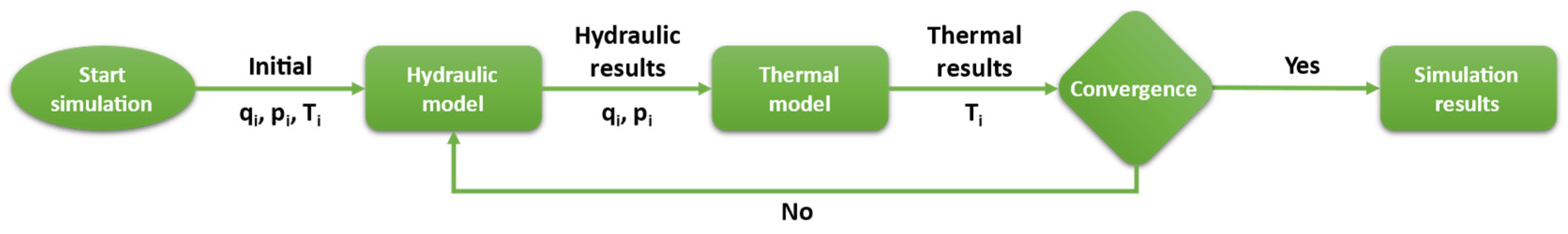
To further simplify the complexity of the model, the coupled network model can be split into two separate physical models, i.e., a hydraulic and a thermal one, which can be alternately solved until convergence. The hydraulic model is solved to provide pressures and flowrates for some temperature estimates, whereas the thermal model leads to the pipeline endpoint temperatures for the pressure and flowrate estimates obtained in the previous step. At convergence, the two models need to be satisfied by a unique set of pressure, flowrate, and temperature values.

More specifically, flowrate, pressure, and temperature initial estimates are introduced to the hydraulic model (generated by the developed algorithm presented in Section 2.4), which, when solved, provides new pressure estimates at every node and flowrate at each element. Those answers are forwarded to the temperature model to output the entry and exit temperatures of each element, which in turn are introduced back to the hydraulic model. The whole process is repeated in a loop until the coupled model parameters converge, thus leading to unique values of pressure, temperature, and flowrate, which satisfy all governing laws. Each one of the distinct models contains its own number of unknowns, the sum of which corresponds to the unknowns of the coupled system. Similarly, the sum of each model’s equations corresponds to those governing the coupled model. The workflow of the coupled model’s circular solution is presented in Figure 2. The exact form, initialization, and solution method of each separate sub-model are discussed in the following sections.

2.1. Hydraulic Network Model

The hydraulic model contains $L+N$ unknowns, namely the rate at each element (L unknowns) and pressure at each node, including both internal and external ones ($N$ unknowns). It comprises $L+I+E=L+N$ equations, that is, one equation of pressure–flowrate for each element ($L$ equations), one mass conservation equation for each internal node ($I$ equations), and an equation for each boundary condition (flowrate/pressure) at each external node/wellheads and delivery point ($E$ equations).

For the steady-state flow of liquid water through a cylindrical pipe, the pressure drop is attributed to friction due to the viscous flow, the roughness of the pipe, and gravity effects due to the elevation difference of the two pipe endpoints. The relation of pressure–flowrate through a pipe can be expressed using the Darcy–Weisbach equation:

$$p_{in}-p_{out}-\lambda ·\frac{L}{D}·\frac{\rho }{2}·{\left(\frac{4·q}{\pi ·D^2}\right)}^2=0$$

(1)

where $p_{in}$ and $p_{out}$ are the pressures at the pipe entry and exit points, $\lambda$ is the pipe friction factor, $L$ is its length, $D$ is the diameter, $\rho$ is the fluid density, and $q$ is the (volumetric) flowrate. The friction factor depends on the type of flow (laminar/turbulent), which is further determined by the Reynolds number ($Re$). For Reynolds numbers below 2320, the flow is laminar, and the friction factor is simply given by:

$$\lambda =\frac{64}{Re}\to \lambda =\frac{16·\mu ·\pi ·D}{q·\rho }$$

(2)

where $\mu$ is the fluid viscosity. For high Reynolds numbers, the flow is turbulent, and $\lambda$ can be estimated by:

$$\frac{1}{\sqrt{\lambda }}=-2·\log \left[\frac{2.51}{Re·\sqrt{\lambda }}+\frac{k}{3.71}\right]$$

(3)

where $k$ is the relative roughness of the pipe.

Gravity effects can be incorporated into the Darcy—Weisbach equation for laminar flow in the form of:

$$p_{in}-p_{out}-\frac{128·\mu ·L·q}{D^4·\pi }+\rho ·g·\left(h_{in}-h_{out}\right)=0$$

(4)

whereas for turbulent flow, it is expressed by:

$$p_{in}-p_{out}-\frac{8·\lambda ·L·\rho ·q·\left|q\right|}{D^5·{\pi }^2}+\rho ·g·\left(h_{in}-h_{out}\right)=0$$

(5)

and $h_{in}$ and $h_{out}$ stand for the elevation of the pipe ends.

At the internal nodes, conservation of mass dictates that the mass of the fluid exiting the internal node equals the mass that enters it. Therefore, for internal node i:

$$\sum _{j\in I_{{arr}_i}}{\dot{m}}_j=\sum _{j\in I_{{dep}_i}}{\dot{m}}_j\Rightarrow \sum _{j\in (I_{{arr}_i}\cup I_{{dep}_i})}{\delta }_j·q_j=0,\hspace{1em}\hspace{1em}1\le i\le I$$

(6)

where $I_{{arr}_i}$ and $I_{{dep}_i}$ are the sets of elements arriving to and departing from node $i$, respectively, ${\delta }_j$ equals to 1 or −1 depending on whether element j is contributing or removing fluid from the node $i$, based on its connectivity.

Boundary conditions are applicable to the external nodes, and they may correspond to fixed pressure or flowrate values. Out of $E$ external nodes, let $E_P$ be the set containing the ones for which a pressure boundary condition $P_i$ is available, whereas $E_Q$ contains the nodes with a flowrate boundary condition $Q_i$. Then, the boundary conditions equations are as follows:

$$p_i-P_i=0,\hspace{1em}\hspace{1em}i\in E_P$$

(7)

$$q_{j\left(i\right)}-Q_i=0,\hspace{1em}\hspace{1em}i\in E_Q$$

(8)

where $j$ is the index of the element connected to external node $i$.

The hydraulic equations for each element and node can be transformed into a system of $L+N$ non-linear equations, which can be easily solved using a numerical method, such as the conventional Newton–Raphson method. It must be noted that Equation (4) is linear in its unknowns, whereas non-linearity appears when turbulent flow is considered (Equation (5)). As shown in Section 3, in the case of real-world geothermal fluids networks, the introduced non-linearity is quite mild and can be easily handled by conventional non-linear equation-solving methods.

2.2. Thermal Network Model

The thermal model utilizes $2L$ unknowns, namely the temperature at the entry and exit points of each element. The model accounts for the conservation of thermal heat flux for each element ($L$ equations), the conservation of energy at each internal node ($I$ equations), and the boundary temperature conditions at each node/wellhead ($E-1$ equations). In total, the thermal model consists of $L+I+E-1=L+N-1=2L$ equations, equal to its number of unknowns.

The fluid’s thermal energy interchange with the environment is dominated by conduction, controlled by the overall heat transfer coefficient $U$, which accounts for the total conductivity of all material layers (pipe steel, liners, insulation, etc.) between the pipeline segment fluid and the outer environment. The energy that gets transferred per unit of time $dT$ and unit of pipe length $dx$ (i.e., heat power per unit length) is equal to:

$$Q_c=U·A·\left({\overline{T}}_{el}-T_{\infty }\right)$$

(9)

where $A$ accounts for the inside area of a pipe per unit of length, ${\overline{T}}_{el}$ is the average temperature of the fluid inside the pipe, $T_{\infty }$ is the outside temperature (ground or air). Heat power loss from the fluid to the pipe body causes a temperature drop of the fluid, which depends on its thermal capacity and is given by Equation (10):

$$Q_o=\dot{m_w}·C_p·\left(T_{in}-T_{out}\right)$$

(10)

where $\dot{m_w}$ is the mass flowrate of the water, $C_p$ is the specific heat capacity of water, $T_{in}$ and $T_{out}$ are the temperatures at the entry and exit points of the pipe.

By equating Equations (9) and (10), the heat power loss in a pipe along a differential length $dx$ is described by the differential Equation (11) [30]:

$$Q_c=Q_o\to \frac{dT}{dx}=-\frac{U·\pi ·D}{\dot{m_w}·Cp}·\left({\overline{T}}_{el}-T_{\infty }\right)$$

(11)

where $D$ is the pipe’s internal diameter. Solving Equation (11), the temperature drop within a pipe of length $L_i$ is now given by the algebraic Equation (12):

$$\exp \left(R_i·L_i\right)·T_{i{n}_i}-T_{ou{t}_i}=[\exp \left(R_i·L_i\right)-1]·T_{\infty },\hspace{1em}\hspace{1em}1\le i\le L$$

(12)

where:

$$R_i=-\frac{U_i·\pi ·D_i}{{\rho }_i·q_i·C_p}$$

(13)

At each internal node, different water flowrates, each at specific pressure and temperature conditions, arrive and depart as they are transferred through the pipes. Conservation of energy at any internal node states that heat entering such a node equals that exiting that node, thus constraining the inlet and outlet temperatures of the connected elements:

$$\begin{gathered} Q_{{arr}_i}-Q_{{dep}_i}=0\Rightarrow \sum _{jϵI_{{arr}_i}}{Q}_j-\sum _{jϵI_{{dep}_i}}{Q}_j=0\Rightarrow \\ \sum _{jϵI_{arr}}\left(q_j·T_{{out}_j}\right)-\sum _{jϵI_{dep}}\left(q_j·T_{{in}_j}\right)=0 \end{gathered}$$

(14)

where $Q_{{arr}_i}$ and $Q_{{dep}_i}$ correspond to the heat amount arriving and departing by geothermal fluids at internal node $i$. $Q_j$ is the heat flowing through element $j$, and $I_{arr}$ is the set of elements arriving at node $i$. Similarly, $I_{dep}$ is the sum of elements $j$ that depart from node $i$. $T_{{out}_j}$ and $T_{{in}_j}$ correspond to the output and input temperatures at the endpoints of elements belonging to $I_{arr}$ and to $I_{dep}$, respectively.

The thermal behavior of the network at each inlet external node is further dictated by the boundary temperature set ($T_i$). The boundary temperature is applied to the inlet temperature of the connected element ($T_{in}$):

$$T_{{in}_j}=T_i,\hspace{1em}\hspace{1em}i\in E_{in}$$

(15)

where $i$ is the external node and $j$ is the element that connects to said node and $E_{in}$ is the inlet external nodes subset.

Equations (12), (14), and (15) can be collected to a system of $2L$ non-linear equations that is solved using any non-linear solver, such as the conventional Newton–Raphson method. It must be noted that Equation (13) utilizes the fluid’s density, which is not a constant, but rather changes depending on its pressure and temperature conditions, which in turn renders Equation (12) as non-linear. However, this behavior is quite mild in the case of real-world geothermal fluids networks, as shown in the Case Study section.

2.3. Fluid Model

The hydraulic and thermal element equations utilize the fluid’s density and viscosity. These fluid properties are not constant but vary with the fluid’s temperature and pressure conditions. To accurately estimate them, a dedicated fluid model needs to be available.

For this study, the 2012 revised release of the International Association for the Properties of Water and Steam Industrial Formulation 1997 (IAPWS-IF97) was used. This formulation is developed for industrial use and recommended for the calculation of thermodynamic properties of ordinary water in its fluid phases, including vapor–liquid equilibrium. The formulation consists of a set of equations, which are valid for the temperature range of 273.15 K to 1073.15 K for pressures up to 100 MPa and for the range of 1073.15 K to 2273.15 K for pressures up to 50 MPa [31].

Figure 3 shows the five regions into which the entire range of validity of IAPWS-IF97 is divided based on the temperature and pressure conditions. Each of the five regions is dictated by its own equation. Regions 1, 2, and 5 are each defined by a fundamental equation for the specific Gibbs free energy, region 3 is limited by a fundamental equation for the specific Helmholtz free energy, and finally, the saturation curve (region 4) is dictated by a saturation–pressure equation [31,32].

2.4. Initialization Algorithm

Numerical methods, such as Newton—Raphson, require appropriate initial conditions to reach the solution. For that reason, an initial values estimation algorithm has been developed.

First, the algorithm runs for all the external inlet nodes in the system. Those nodes, i.e., the wellheads, are connected on one end with an element, and each one contains a flowrate and a temperature boundary condition. The algorithm then sets the initial flowrate and the initial inlet temperature value of those elements equal to the flowrate and the temperature boundary condition of the wellhead that they are connected to. Once all boundary temperature conditions have been assigned to their corresponding elements, the value of a random boundary temperature condition is assigned to the rest of the initial input/output temperature conditions. The initial pressure value of the end node is set equal to the boundary pressure value set at the delivery point.

To estimate the initial flowrate values for the internal nodes, the algorithm runs a check to determine which elements contribute fluid to the node and which ones remove fluid from it. The check is performed based on element connectivity if the internal node is referenced first and then, the element is considered as an outlet; alternatively, the element is considered as an inlet point. Starting from elements connected to the wellheads (which have already been assigned initial values), the algorithm checks the flowrates of the elements that act as inputs to the internal node, sums the values, and distributes them equally to its output elements.

For every internal node, a check is performed on its input and output elements. If the input node of the input element that is being checked already has an initial pressure condition, then 90% of that value is assigned as the initial pressure condition of the internal node. If none of the input elements fit the criteria above, then the same check is performed on the output node of the output elements, in which case the internal node’s initial pressure condition is set to 110% of the value of the output node.

2.5. Software Implementation

To implement the surface pipeline model, a Python algorithm has been developed. Python’s ability to utilize fast and dedicated libraries for numerical calculations and specialized modules (like the fluid model IAPWS-IF97) or ports of developed algorithms, like the initialization one, makes it ideal for complex simulation applications, resulting in a CPU-time requirement for a complete simulation run to be in the order of milliseconds on a regular PC.

To perform a complete simulation, the only inputs that are required from the user are the number of nodes and elements of the network, the nodes’ coordinates, the pipelines’ connectivity, and their design characteristics (diameter, roughness, and thermal conductivity). The model can handle any user-defined geometry, given the aforementioned inputs by utilizing a developed algorithm.

First, the algorithm identifies which nodes are external (wellheads and delivery point) and which ones are internal (junctions). To perform this characterization, the algorithm checks the connectivity of each element, which is defined by a pair of two nodes, arbitrarily handled as input and output nodes of the equivalent element. This procedure also defines an initial flow direction estimate through that pipeline. The nodes that are identified as being connected to an element only once, and thus used only once as an input or an output, are classified as external nodes; otherwise, they are characterized as internal nodes. Furthermore, if the external nodes have been identified as an input to their element, they are classified as wellheads; otherwise, that node is the delivery point. Proper flow direction is based on the results of the simulation. If the correct flow direction was initially set by the user, then, the results of the flowrate would be positive. Inverse flow would be signified by a negative flowrate value for the pipeline that was initially set wrong. Lastly, the elevation difference between the input and the output of each pipeline is calculated as the difference of its nodes’ Z-coordinates, and the pipeline length is calculated as the Euclidean norm between its nodes’ X-, Y-, and Z-coordinates.

To ensure that proper network geometry has been set, the algorithm also validates the user inputs to ensure proper functionality of the simulation. First, it checks if the number of nodes exceeds the number of elements by one, given that each pipe needs an entry and an exit point. Then, the algorithm validates that a correct number of boundary conditions has been set according to the requirements described in Section 2.1 and Section 2.2. If at any point, there is an issue with user input, the algorithm terminates the code before the simulation begins, promptly informing the user of the input errors so that they can update them and rerun the code.

3. Case Study and Results

3.1. Case Study Setup

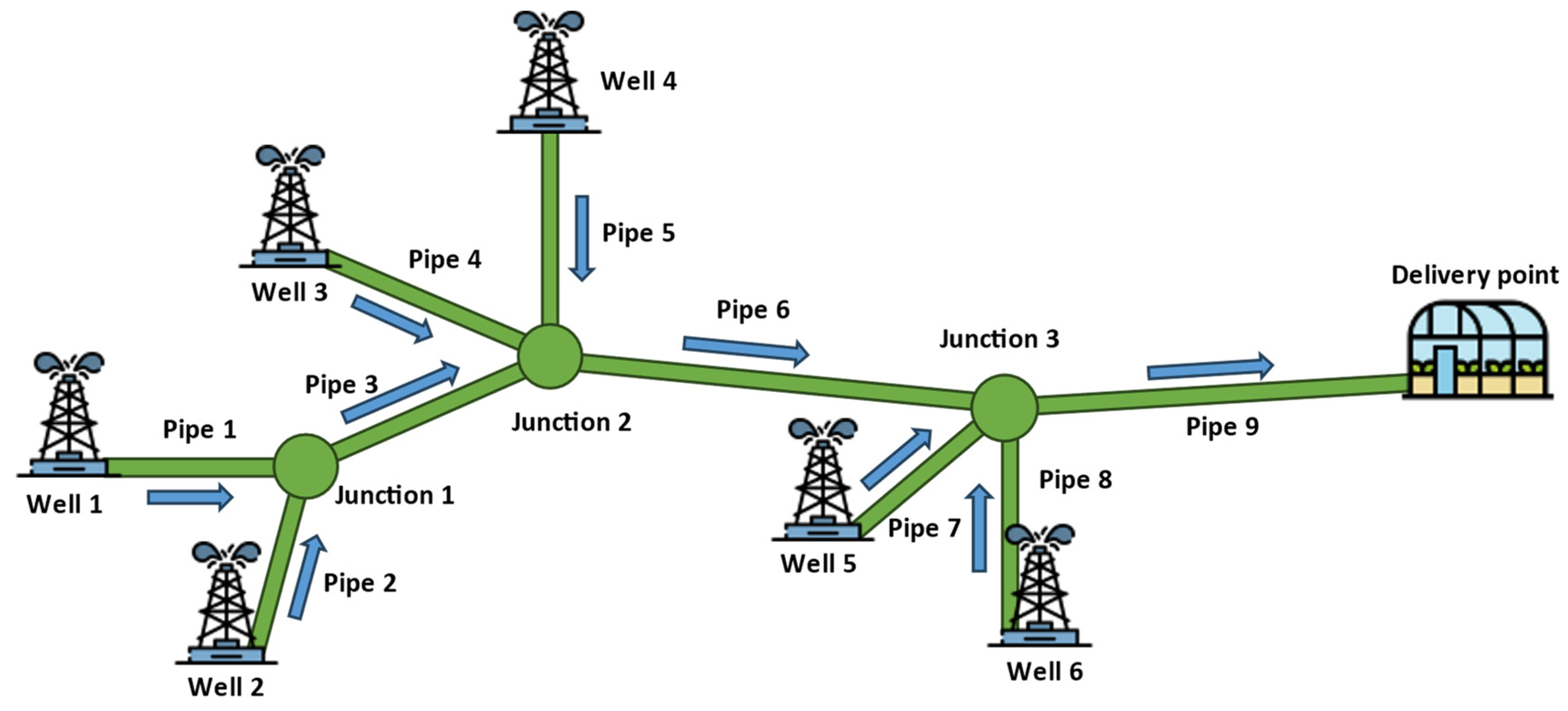
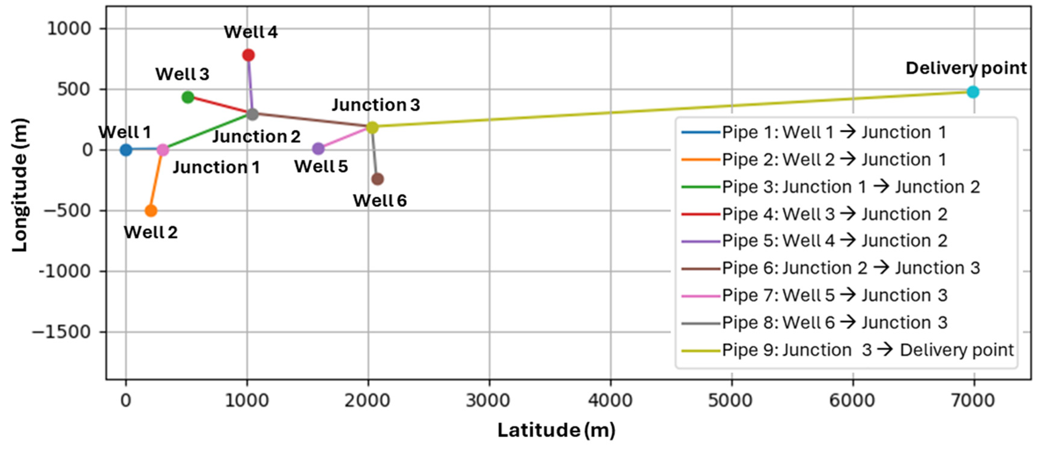
To demonstrate the proposed model structure and solution, a real-world Northern Greek low-enthalpy geothermal field was tested, comprising three well pairs, which deliver about 46 GWH_th, utilizing geothermal fluids of 70–80 °C. The produced geothermal fluid from each well pair was driven to a dedicated junction on the main pipeline network. Each well was connected to its corresponding junction via a dedicated pipe, and the network ultimately directed the commingled fluid to a greenhouse, i.e., to the delivery point. In total, six wells draining different parts of the geothermal resource contributed fluids at different temperatures, and the ending flow was directed to the delivery point (Figure 4 and Figure 5). The network covered an area of 8.95 km² with 9527.8 m of pipelines, with the furthest two points in the network (from wellhead 2 to the delivery point) being 7.3 km apart and exhibiting a maximum inclination of 6.6 m.

The goal was to solve the steady-state flow problem under various construction and operating conditions to maximize the produced enthalpy at the delivery point, while also maintaining the client’s requirement for a fixed output pressure, set to 5 bar in that case. All physical constraints such as avoiding backflow, fluid choking, and excessive heat loss needed to be satisfied by the obtained solution.

Fundamentally, the field’s geometry can be described as a system of 10 nodes, of which 7 are external (6 wellhead entry nodes and 1 delivery point end node) and 3 are internal (junctions), interconnected through nine elements/pipes. Therefore, the following unknowns need to be determined by the simulation:

• Flowrate at each element (nine unknowns in total)
• Pressure at each node (10 unknowns in total)
• Input and output temperatures at each element (18 unknowns in total)

The design problem contains 37 unknowns, 19 of which are incorporated in the hydraulic model (elements’ flowrates and nodes’ pressures), whereas the remaining 18 are contained in the thermal model (elements’ input and output temperatures).

To complete the system description, seven boundary conditions are needed. First, six boundary flowrates and six boundary temperatures must be defined, two at each wellhead. It must be noted that these conditions correspond to the properties of the fluids that arrive at the wellheads; they are expected to be obtained from the reservoir and wellbore models or directly from the wellhead monitoring systems, and they are imposed on the surface network model by boundary conditions [33]. Additionally, one boundary pressure condition at the end node needs to be set as this pressure, corresponding to the pressure target at the delivery point, and is adjusted by the operator. The network’s geometry and boundary parameters of the external nodes are given in detail in

Table 1. Network geometry and boundary parameters.

Nodes	Coordinates (m)			Flowrate (m3/h)	Temperature (°C)	Pressure (Bar)
	X	Y	Z
Well 1 (W1)	0.0	0.0	0.0	63.55	89.82	-
Well 2 (W2)	205.1	−498.7	−1.8	65.34	87.34	-
Well 3 (W3)	513.2	437.6	2.8	52.76	81.48	-
Well 4 (W4)	1016.7	783.4	4.4	53.71	79.74	-
Well 5 (W5)	1588.3	5.4	0.5	51.92	75.19	-
Well 6 (W6)	2074.3	−241.9	−2.2	56.38	73.61	-
Junction 1 (J1)	307.9	2.8	0.9	-	-	-
Junction 2 (J2)	1051.0	296.8	1.0	-	-	-
Junction 3 (J3)	2036.3	187.2	0.9	-	-	-
Delivery Point (DP)	6987.6	472.6	0.1	-	-	5.00

.

In summary, the coupled model is described mathematically by the following set of equations:

• The hydraulic model consists of 19 equations:
  • A pressure–flowrate equation for each element (nine equations in total)
  • A conservation of mass equation for each internal node (three equations in total)
  • A flowrate or pressure boundary condition at the external nodes (seven equations in total)
• The thermal model is defined by 18 equations:

  4.

  A thermal heat flux conservation for each element (nine equations in total)

  5.

  A conservation of energy for each internal node (three equations in total)

  6.

  A temperature boundary condition for the wellheads (six equations in total)

In conclusion, the coupled model of the case study is described by 37 equations, equal to the total number of unknowns in the system.

According to the initial system design, all pipelines were made from the same material. Due to the temperature and pressure conditions typically expected at the wellhead (70–90 °C and <30 bar), steel Schedule 40 pipes, welded and seamless, with a polypropylene liner, uniform roughness of 0.061 mm, and diameter of 100 mm [18], were chosen to protect them from corrosion [34]. The ambient air temperature was set at −5 °C to simulate winter conditions commonly encountered in Northern Greece, hence simulating maximum insulation losses, and the ground temperature was set at 15 °C.

3.2. Scenario 1: Surface-Installed Uninsulated Pipes with 100 mm Diameter

Scenario 1 was set up to simulate a very rough design where only moderate-diameter pipelines (100 mm) equipped with very limited insulation were considered. Such a scenario would correspond to a minimum investment cost, and the impact on the system performance remained to be estimated. According to this scenario, all pipelines were assumed to be installed at the surface, bearing no thermal insulation, which was modeled with an overall heat transfer coefficient as high as 5 BTU/h/ft²/°F, a typical value for an uninsulated steel pipe with a polypropylene liner. This, coupled with the fact that the pipes are installed at the surface, i.e., they are exposed to a cold winter environment at −5 °C, is expected to result in a high heat power loss across the network.

The simulation results detailed in

Table 2. Pressure, flowrate, temperature, and enthalpy results per network node for scenario 1.

Node	Pressure (bar)	Flowrate (m3/h)	Temperature (°C)	Power (MW)
W1	26.03	63.55	89.82	-
W2	27.24	65.34	87.34	-
W3	11.77	52.76	81.48	-
W4	11.47	53.71	79.74	-
W5	−47.40	51.92	75.19	-
W6	−47.07	56.38	73.61	-
J1	24.58	128.89	84.02	-
J2	10.22	235.36	77.35	-
J3	−48.90	343.66	73.01	-
DP	−680.38	343.66	64.79	-

display various issues within the system nodes and pipes. This design exhibited significant hydraulic and thermal flaws, with the most prominent being a backflow problem along pipes 6, 7, 8, and 9, as indicated by the negative pressure values at one junction point (J3), two wellheads (W5, W6), and the delivery point (DP). Moreover, the estimated pressure and temperature drop gradients ($\Delta p/\Delta L$ and $\Delta T/\Delta L$ respectively) shown in

Table 3. Flowrate, input and output temperature, pressure, and heat losses for scenario 1 pipelines.

Pipe	Flow Direction			D (mm)	U (BTU/h/ft2/°F)	q (m3/h)	Tin (°C)	Tout (°C)	Δp/ΔL (bar/km)	ΔT/ΔL (°C/km)
Pipe 1 (Surface)	W1	→	J1	100	5.0	65.34	87.34	81.83	5.19	10.76
Pipe 2 (Surface)	W2	→	J1	100	5.0	128.89	84.02	79.85	17.97	5.22
Pipe 3 (Surface)	J1	→	J2	100	5.0	52.76	81.48	74.66	2.79	12.27
Pipe 4 (Surface)	W3	→	J2	100	5.0	53.71	79.74	73.99	2.56	11.80
Pipe 5 (Surface)	W4	→	J2	100	5.0	235.36	77.35	74.71	59.63	2.66
Pipe 6 (Surface)	J3	→	J2	100	5.0	51.92	75.19	69.56	3.11	11.65
Pipe 7 (Surface)	J3	→	W5	100	5.0	56.38	73.61	69.08	4.25	10.53
Pipe 8 (Surface)	J3	→	W6	100	5.0	343.66	73.01	64.79	127.33	1.66
Pipe 9 (Surface)	DP	→	J3	100	5.0	65.34	87.34	81.83	5.19	10.76

indicate that the primary pipeline network suffered from substantial pressure drop, as can be seen from the high gradient values across the whole pipeline network and especially at the main pipeline (pipes 3, 6, and 9). Additionally, pipes 6 and 9 show an unrealistically high pressure gradient (the total pressure drop along pipe 6 was larger than the available pressure at J2), indicating that backflow occurred before Junction 3. Insufficient geothermal fluid pressure was also observed at the third junction, as indicated by the negative pressure value at J3. The flowrate results after J3 were calculated for mathematical purposes only; they were completely unreliable and not representative of reality at all, which is also the reason that the produced enthalpy at the DP was not calculated for scenario 1 and thus, is not shown in Table 2. Finally, the excessively high values of the $\Delta T/\Delta L$ index signify substantial heat losses within the network, and especially along pipes 1, 2, 4, 5, 7, and 8, which distributed the fluid from the wellheads to the mainline.

These results show that it is imperative to first undertake a hydraulic redesign to address these issues before addressing the system’s heat power loss.

3.3. Scenario 2: Surface-Installed Increased-Diameter Uninsulated Pipes at the Mainline

To address the backflow issues, modifications were made to the main network line, comprising the pipes linking the three junctions together with the pipe segment leading to the delivery point, in order to compensate for the excessive pressure drop caused by the high flowrate, according to Equation (5). More specifically, to drastically compensate for the unrealistic pressure losses, the mainline pipe diameter was increased to 200 mm. The pipeline parameters were reset, and the coupled hydraulic and thermal problems were resolved utilizing the modified system properties.

This redesign effectively resolved the backflow problem as shown by the simulation results, elaborated in

Table 4. Pressure, flowrate, temperature, and enthalpy results per network node for scenario 2.

Node	Pressure (Bar)	Flowrate (m3/h)	Temperature (°C)	Power (MW)
W1	25.90	63.55	89.82	-
W2	27.11	65.34	87.34	-
W3	25.59	52.76	81.48	-
W4	25.29	53.71	79.74	-
W5	23.90	51.92	75.19	-
W6	24.23	56.38	73.61	-
J1	24.45	128.89	83.98	-
J2	24.04	235.36	75.10	-
J3	22.40	343.66	69.78	-
DP	5.00	343.66	54.72	21.60

and

Table 5. Flowrate, input and output temperature, pressure, and heat losses for scenario 2 pipelines.

Pipe	Flow Direction			D (mm)	U (BTU/h/ft2/°F)	q (m3/h)	Tin (°C)	Tout (°C)	Δp/ΔL (bar/km)	ΔT/ΔL (°C/km)
Pipe 1 (Surface)	W1	→	J1	100	5.0	63.55	89.82	86.24	4.71	11.63
Pipe 2 (Surface)	W2	→	J1	100	5.0	65.34	87.34	81.79	5.18	10.84
Pipe 3 (Surface)	J1	→	J2	200	5.0	128.89	83.98	75.78	0.52	10.27
Pipe 4 (Surface)	W3	→	J2	100	5.0	52.76	81.48	74.6	2.79	12.37
Pipe 5 (Surface)	W4	→	J2	100	5.0	53.71	79.74	73.94	2.56	11.89
Pipe 6 (Surface)	J2	→	J3	200	5.0	235.36	75.1	70.01	1.65	5.13
Pipe 7 (Surface)	W5	→	J3	100	5.0	51.92	75.19	69.51	3.11	11.75
Pipe 8 (Surface)	W6	→	J3	100	5.0	56.38	73.61	69.06	4.25	10.56
Pipe 9 (Surface)	J3	→	DP	200	5.0	343.66	69.78	54.72	3.51	3.04

for nodes and pipes, respectively, which demonstrate the successful delivery of geothermal fluid to the greenhouse at the desired pressure specified by the client. This design allowed an enthalpy production at a commendable value of 21.60 MW.

Doubling the pipe diameter resulted in a significant reduction in pressure loss within the primary pipeline network. Specifically, the pressure drop along pipe 3 was reduced from 17.97 bar/km to 0.52 bar/km, and the previously unrealistic loss along pipes 6 and 9 presented a healthy drop of 1.65 bar/km and 3.51 bar/km, respectively. However, heat loss across the whole network persisted at elevated levels, as anticipated from the large temperature difference between the warm fluid traveling along the uninsulated pipelines and the cold ambient environment. The most severe heat loss (10–12 °C/km) appeared across pipes 1, 2, 4, 5, 7, and 8, which link the wellheads to the mainline and are attributed to the high wellhead fluid temperature. The first section of the mainline (pipe 3) exhibited a lower flowrate value compared to the rest of the sections (pipes 6 and 9), which means that the fluid flowed through it with less velocity and therefore, had more time to react with the cold environment and exchange heat with it. This justifies the increased value of $\Delta T/\Delta L$ (10.27 °C/km), which is evident in pipe 3 compared to pipes 6 and 9 (5.13 °C/km and 3.04 °C/km, respectively).

Further redesigning efforts were necessary to rectify the thermal deficiencies in the network.

3.4. Scenario 3: Underground-Installed Uninsulated Pipes with 200 mm Diameter at the Mainline

To mitigate the escalating heat loss within the system, an assessment was conducted to explore the possibility of installing the pipelines underground. This strategic placement aimed to capitalize on the naturally occurring higher ambient underground temperature, compared to the colder aboveground temperatures. In real-life scenarios, the ground temperature is expected to stay constant at approximately 15 °C all year long, regardless of the prevailing surface conditions, at a depth of about 1 m below the surface.

The simulation results, shown in

Table 6. Pressure, flowrate, temperature, and enthalpy results per network node for scenario 3.

Node	Pressure (bar)	Flowrate (m3/h)	Temperature (°C)	Power (MW)
W1	25.81	63.55	89.82	-
W2	27.02	65.34	87.34	-
W3	25.5	52.76	81.48	-
W4	25.2	53.71	79.74	-
W5	23.82	51.92	75.19	-
W6	24.15	56.38	73.61	-
J1	24.36	128.89	84.96	-
J2	23.95	235.36	77.26	-
J3	22.32	343.66	72.45	-
DP	5.00	343.66	60.92	23.96

and

Table 7. Flowrate, input and output temperature, pressure, and heat losses for scenario 3 pipelines.

Pipe	Flow Direction			D (mm)	U (BTU/h/ft2/°F)	q (m3/h)	Tin (°C)	Tout (°C)	Δp/ΔL (bar/km)	ΔT/ΔL (°C/km)
Pipe 1 (Underground)	W1	→	J1	100	5.0	63.55	89.82	86.99	4.70	9.18
Pipe 2 (Underground)	W2	→	J1	100	5.0	65.34	87.34	82.99	5.18	8.50
Pipe 3 (Underground)	J1	→	J2	200	5.0	128.89	84.96	78.52	0.52	8.06
Pipe 4 (Underground)	W3	→	J2	100	5.0	52.76	81.48	76.19	2.79	9.52
Pipe 5 (Underground)	W4	→	J2	100	5.0	53.71	79.74	75.3	2.56	9.09
Pipe 6 (Underground)	J2	→	J3	200	5.0	235.36	77.26	73.32	1.65	3.98
Pipe 7 (Underground)	W5	→	J3	100	5.0	51.92	75.19	70.92	3.11	8.83
Pipe 8 (Underground)	W6	→	J3	100	5.0	56.38	73.61	70.22	4.25	7.88
Pipe 9 (Underground)	J3	→	DP	200	5.0	343.66	72.45	60.92	3.49	2.33

, demonstrate the success of this redesign in reducing heat loss throughout the network, especially across the main pipeline, resulting in an overall increase in the fluid’s temperature by 1, 2, and 3 °C in junctions 1, 2, and 3, respectively. Heat loss remained more prominent across pipes 1, 2, 3, 4, 5, 7, and 8, as was the case with scenario 2, but it was uniformly reduced by 2.2–2.9 °C/km. Consequently, the geothermal fluid arrived at the delivery point at a significantly higher temperature (60.92 °C compared to 54.72 °C).

As a result of this adjustment, additional power was produced, which amounted to 23.96 MW, an improvement over the previous design’s 21.60 MW (11% increase).

3.5. Scenario 4: Underground-Installed Insulated Pipes with 200 mm Diameter at the Mainline

Although the outcomes of scenario 3 exhibited significant improvement over the former ones, the network was not fully optimized before addressing the effect of adding insulation to the network pipes. To explore this, the overall heat transfer coefficient value of the formerly uninsulated pipelines, set at 5 BTU/h/ft²/°F, was adjusted to 1 BTU/h/ft²/°F for the insulated ones. This value corresponded to a moderately insulated pipeline. The most common pre-insulated pipe material was steel, which was covered with a layer of polyurethane foam on the inside, with a thickness of 40 mm and a thermal conductivity of 0.18 BTU/h/ft²/°F/in and protected from moisture by a PVC jacket, according to the European minimum standard of 3.175 mm of thickness and a thermal conductivity of 1.2 BTU/h/ft²/°F/in [5,34,35].

The results of the simulation, depicted in

Table 8. Pressure, flowrate, temperature, and enthalpy results per network node for scenario 4.

Node	Pressure (Bar)	Flowrate (m3/h)	Temperature (°C)	Power (MW)
W1	25.59	63.55	89.82	-
W2	26.79	65.34	87.34	-
W3	25.28	52.76	81.48	-
W4	24.98	53.71	79.74	-
W5	23.62	51.92	75.19	-
W6	23.94	56.38	73.61	-
J1	24.14	128.89	87.84	-
J2	23.73	235.36	83.37	-
J3	22.12	343.66	79.69	-
DP	5.00	343.66	76.91	29.97

and

Table 9. Flowrate, input and output temperature, pressure, and heat losses for scenario 4 pipelines.

Pipe	Flow Direction			D (mm)	U (BTU/h/ft2/°F)	q (m3/h)	Tin (°C)	Tout (°C)	Δp/ΔL (bar/km)	ΔT/ΔL (°C/km)
Pipe 1 (Underground)	W1	→	J1	100	1.0	63.55	89.82	89.26	4.70	1.83
Pipe 2 (Underground)	W2	→	J1	100	1.0	65.34	87.34	86.46	5.17	1.71
Pipe 3 (Underground)	J1	→	J2	200	1.0	128.89	87.84	86.47	0.51	1.72
Pipe 4 (Underground)	W3	→	J2	100	1.0	52.76	81.48	80.4	2.78	1.94
Pipe 5 (Underground)	W4	→	J2	100	1.0	53.71	79.74	78.84	2.55	1.85
Pipe 6 (Underground)	J2	→	J3	200	1.0	235.36	83.37	82.49	1.63	0.88
Pipe 7 (Underground)	W5	→	J3	100	1.0	51.92	75.19	74.33	3.10	1.78
Pipe 8 (Underground)	W6	→	J3	100	1.0	56.38	73.61	72.92	4.24	1.60
Pipe 9 (Underground)	J3	→	DP	200	1.0	343.66	79.69	76.91	3.45	0.56

, show that the addition of insulation to the pipelines drastically reduced the heat loss across the underground pipes, especially across the main pipeline, resulting in an overall increase in the fluid’s temperature by 3, 6, and 7 °C in junctions 1, 2, and 3, respectively. $\Delta T/\Delta L$ was reduced by 6.3–7.6 °C across pipes 1, 2, 3, 4, 5, 7, and 8, resulting in an overall low heat loss of the range 0.561–1.935 °C/km.

Consequently, the geothermal fluid reached the delivery point at an even higher temperature, leading to a notably increased power production of 29.96 MW (25% increase compared to scenario 3 and 39% compared to scenario 2).

4. Discussion

For all scenarios, the coupled (hydraulic and thermal) model fully converged after only two iterations of the outer loop (Figure 2). This implies that the model’s algorithm is fast, robust, and efficient at converging to the solution of the simulation problem. This behavior comes down to the effectiveness of the initial parameter estimation and the overall near non-linearity of the problem. The flow throughout the network was turbulent; therefore, the hydraulic model utilized the non-linear Equation (5) for each element. However, the very few iterations required for the full convergence of the coupled simulation problem are justified by the fact that the inner hydraulic and thermal problems exhibited only limited non-linear behavior. It is noted that if the flow was laminar, and therefore, the hydraulic model utilized the laminar expression of the Darcy–Weisbach equation (Equation (4)), then, the coupled problem would be almost fully linear (apart from the loose dependency of density and viscosity on temperature), and the solution would result after a single iteration. Furthermore, the effectiveness of the initialization algorithm is shown by the fact that the Newton–Raphson method used to solve the simulation effectively utilizes values that are close enough to the actual solution. This observation is true only when the fluid is liquid, and this behavior is attributed to its very limited compressibility. Obviously, in a network transporting two-phase fluid or single-phase steam, the behavior would be different, and the pressure drop would be greater, thus introducing the need to incorporate an Equation of State in the developed equations.

Each scenario is characterized by different design conditions, such as pipeline diameter, insulation, and installation type, with the only constants across the four variants being the boundary conditions of flowrates and temperatures at the wellhead and the pressure requirement at the delivery point since the latter depends on the reservoir and wellbore performance. Each system variation resulted in different enthalpy being produced at the delivery point, and the different system specifications directly impacted pressure and heat losses across the network.

To achieve the calculated results, the specific calculated pressure conditions were imposed on the network. However, while temperature is naturally derived directly from the reservoir, via the wellbores, wellhead pressures, and thus, the flowrates, can be controlled by the operator either by choking or by pumping the wells. Indeed, a fully developed geothermal system has two control points available to regulate flow once it has been designed and delivered: the pumps and the chokes. If the pressure is not enough at the wellhead to achieve optimal operation, pumps need to be installed to provide the additional pressure needed in the system. On the other hand, if the wellhead presents pressure higher than the one needed to meet the client’s requirements at the delivery point, production can be controlled by operating the chokes, thus reducing the available pressure at the wellheads. If those conditions are altered by the field operator, the network needs to be solved again and the obtained solutions need to be used to globally optimize the geothermal fluid production system.

The economic viability of the scenarios is crucial for the project’s feasibility and sustainability. The varying scenarios, with distinct pipeline materials, diameters, insulation strategies, and installation methods, necessitate detailed economic analyses. The mathematical model is a designing tool; however, in-depth cost estimates, including construction, materials, installation, and operational expenses, are essential for the economic group. These analyses, typically implemented in business models, should account for factors such as power output, operational cost, potential revenue streams, return on investment, and life cycle costs. The software’s flexibility in performing redesigns allows the economic group to validate and update cost estimates promptly and effectively.

The developed tool ensures that economic stakeholders receive comprehensive and relevant information to guide their decision-making processes effectively, which ultimately helps them arrive at a safe Final Investment Decision (FID).

5. Conclusions

The developed mathematical model successfully simulates a surface pipeline geothermal fluids network, which, due to its complex geometry, mathematically requires a large number of unknowns and an equal number of equations to be solved. Decoupling the full model into two separate models, i.e., a hydraulic and a thermal, to simplify the solving process, and then recoupling them, by solving them iteratively, proved to be successful and efficient.

The initial values estimation algorithm consistently provides safe and close estimates to the calculated results, allowing the Newton–Raphson method to operate efficiently without convergence issues and with very few iterations. The results obtained demonstrate reasonable pressure drop and heat loss along each pipe, aligning with expectations.

Quick convergence and a few required iterations confirmed that, for cases of turbulent geothermal fluid flow in low-middle enthalpy geothermal field networks, non-linearity in the problem of simulation is observed. However, it was demonstrated that this behavior is limited, resulting in rapid convergence when methods for non-linear problems are applied.

The developed model succeeded in its role as a reliable design tool that offers engineers and the economic group the ability to perform and analyze a vast number of unique scenarios, utilizing different possible parameters rapidly and efficiently. This process makes identifying and solving problem limitations of the network a quick task and helps with the FID from the management. Ultimately, integration with a reservoir and a wellbore simulator, is the next development step to estimate the flow of the geothermal fluid from the reservoir to the delivery point, while considering all flow subsystems contributing to the field exploitation.