Abstract
The short and long-range orders in alloys can be assessed based on a new expression for the combinatorial factor, which is more convenient and intuitive than the traditionally used form. This novel expression can be directly applied to reproduce the results of several well-known statistical-thermodynamic models that are typically considered independent or even inconsistent. The short list of models includes Quasichemical Theory, Associated Solution Model, Surrounded Atom Model, and Cluster Site Approximation. As a result, the formalism and interpretation of these models are significantly clarified, allowing us to identify and fix several long-standing errors that might otherwise have gone unnoticed. Multicomponent generalization of these models is also greatly simplified. For systems undergoing a phase transition, an extended version of the theory provides a mechanism that allows the correct critical temperature of phase transition to be reproduced, as well as a significant increase in the accuracy of thermodynamic functions. In the case of order–disorder transformations, the new theory ensures an integrated description of short and long-range orders, which has long been considered an important and difficult problem.
1. Introduction
The great variety in the thermodynamic properties of multicomponent solutions is responsible for the abundance of model theories called upon to describe such systems. Even in the simple case of metal-like substitutional mixtures the short list includes Cluster Variation Method (CVM) [1], Quasichemical Theory (CT) [2], Associated Solution Model (ASM) [3], Surrounded Atom Model (SAM) [4], Cluster Site Approximation (CSA) [5].
The listed models are successfully used, among other things, to describe systems with moderate differences in the properties of the components that do not lead to the redistribution of atoms over the sites of several interpenetrating lattices. At the same time, it is natural to expect that even small differences in the energy of the interatomic interaction of the components should cause local deviations in the arrangement of atoms from a random order. Such deviations are described usually mathematically by the Warren–Cowley Short-Range Order (SRO) parameter [3,6].
If the differences in the properties of components become stronger, system with negative deviations from ideality may experience transaction to multigrid state that require usage of Long Range Order (LRO) [7] parameter. The commonly used method to describe such systems is the Compound Energy Formalism (CEF) [7]. Unfortunately CEF in its classical form completely neglects SRO. There have been multiple attempts [8] to model SRO as an artificial addition to the basic CEF formalism but this approach has met significant problems. First of all, this implementation introduces SRO as an independent contribution and therefore such an approach neglects the genetic relations between LRO and SRO that exist at the atomic level. Second, SRO modeling is usually achieved by adding artificial mathematical expression (typically, presented as polynomial in alloy concentration) to the CEF expression for the free energy and it is very difficult to ensure the correct behavior of this expression at very high or very low temperatures. This brings CEF outside of the scope of this article because SRO is our primary subject in this article.
We must also remember that there are actually several types of SRO [6]. We are particularly interested here in the chemical SRO [9], which describes local deviations in the number of atoms of various components from the average. Topological SRO describes the displacement of atoms from their local equilibrium positions and is outside of our attention.
There is a clear consensus on the substantial role of SRO in the thermodynamics of liquid and solid alloys [8,9,10,11]. At the same time, the accurate description of SRO presents evident mathematical challenges confirmed by the fact that we do not have a commonly accepted method to take this phenomenon into account. The most advanced way to handle this task is the Cluster Variation Method [1], which allows us to take into account both short and long-range orders and their interrelation. Unfortunately, the use of this method is limited due to its computational complexity, which increases exponentially with the number of components.
The already mentioned short-range parameters [2,6,9] are widely used to describe the elements of SRO accessible from diffraction experiments, but, unfortunately, provide merely a one-dimensional picture of SRO. Such an approach turns out to be quite suitable for the correct calculation of the energy of a simple alloy, but can hardly be considered sufficient when considering the entropy of the system. With such a description, the details of the three-dimensional arrangement of atoms, which are equally important for understanding the structure of the alloy and which directly affect the entropy and other properties, remain hidden. This is also true for the already mentioned popular Warren–Cowley SRO parameter.
The importance of taking into account the three-dimensional form of the distribution of atoms in comparison with the one-dimensional description supported by the standard SRO parameters can be illustrated by a simple example. One-dimensional description of SRO is implemented inside the quasichemical theory (QT) just by taking in the account the number of pairs of type [2]. The free energy of the alloy in the framework of this simple theory depends only on two model parameters: the binding energy of two adjacent atoms a and b and the coordination number z of the lattice. This means that, within the framework of QT, two alloys with the same coordination number are thermodynamically indistinguishable if the energy of atom interaction is the same.
To test this prediction of QT we can consider two systems having the same coordination number : 2D triangular and 3D simple cubical lattices. Rather than being termodynamically indistinguishable, these two system exhibit pronounced differences: near the critical point the simple cubical lattice has a configurational entropy that is nearly 40% greater than the entropy of the triangular lattice [12].
To correctly model such differences, we must consider configurations of atoms that exist in three dimensions but are not possible in two dimensions. This goal can be achieved by including groups of atoms containing at least four atoms, since three atoms cannot be considered as a three-dimensional object. This approach is used in the Cluster Variation Method [1], the most advanced model in thermodynamics of alloy, which, unfortunately, as discussed above, cannot be widely applied. As result, we have an abundance of attempts to take SRO into the account within the framework of model theories [3,4]. Model theories try to represent SRO by directly modeling the allocation of components within small groups of atoms, and then by calculating how this allocation changes the energy and entropy of the alloy. The collected information is used to predict the thermodynamics of the system as a whole.
The described scenario, in which we deduce the thermodynamics of the entire system by just modeling the local atoms arrangement is so typical that it can be used to describe the corresponding theories from some general point of view. The purpose of this article is to show that although the above-mentioned theories such as Quasichemical Theory [2], Associated Solution Model [3], Surrounded Atom Model [4], Cluster Site Approximation [5] (to name just a few best known) are usually presented in intentionally incompatible forms, they still have a common basis that allows us to treat these models as part of some general approach.
Theory of Inhomogeneous Short-Range Order (TISR) [13,14,15] was just developed as an attempt to present the thermodynamics of alloy through the properties and relative amounts of small groups of atoms (cells, as they will be referred to in the following text) conventionally selected in the system, and in this respect is very similar to the listed model theories. It is distinct, however, in several aspects, and it is important to recognize the most significant differences when reading this report.
First, a new form of treatment for combinatorial problems will be provided. It is more intuitive than, for example, the methods traditionally used by the quasichemical theory, and, besides, presents the combinatorial factor (CF) [9] in a form that simplifies the multicomponent generalizations.
Second, a new set of variables will be used to express the properties and composition of an alloy in a parametric form. The use of these variables can greatly simplify mathematical formalism.
Third, all versions of the formalism will be evaluated by comparison with the results presented for the Ising model in [12], to be sure that an acceptable level of precision can be ensured. This step is vital for eliminating the errors in the CF made by some well known model theories, as shown below.
The unusual term “cell” instead of the usual “cluster” is used in this article intentionally to distinguish between a cluster as physical entity and a cell as a formal imaginary construct introduced for computational purposes. The presentation of alloy as a conglomerate of cells has many technical advantages. Each cell makes some contribution to the energy of the system. The permutations of atoms within the cells and rearrangements of cells as a whole are responsible for the configurational entropy of mixing. At the same time, knowledge of atom allocation inside every cell can be considered as a specific form of SRO presentation in the vicinity of this cell.
When SRO is understood in this sense, it also suggests that SRO varies from cell to cell. The term “inhomogeneous” in the name of theory just emphasizes that the model takes into account these local variations of SRO. The standard short-range parameters [2,6,9] use the averaged form of this information and therefore can be used for energy evaluation only. The ability to calculate the configurational entropy is lost, and usually it means that the crude Bragg–Williams [2] approximation has to be used instead.
TISR shares the described form of SRO presentation with all the previously mentioned model theories and, consequently, can be directly applied to reproduce all the results of these theories, if the cells are selected accordingly.
We will see that the developed approach accurately reproduces the results of few models, such as CT and CSA, and significantly improves ASM and SAM by identifying and correcting blunders in these models that have gone undetected for many years.
At the same time, an integrated approach makes it possible to significantly improve the accuracy of all models under consideration with the help of a patch, which has so far only been applied inside the CSA. In general, the unification achieved through the application of the proposed method provides advantages that should not be underestimated.
The structure of the main text is as follows:
The basic formalism or TISR is presented in Section 2 with immediate application to the ordinary quasichemical theory in Section 3.
The Section 4 presents improved version of CF that allows to ensure correct critical temperature to be enforced in every of the model considered in the text.
In the following sections the formalism presented in Section 2, Section 3 and Section 4 is applied to remaining cases:
Although every one of the listed in Section 3, Section 4, Section 5, Section 6, Section 7 and Section 8 cases has some specificity, the structure and the logic used to develop the listed partial cases remains mostly unchanged. Accordingly, some of the corresponding sections (in particular, the Section 5, Section 6, Section 7 and Section 8) may be omitted on first reading.
2. Theory of Inhomogeneous Short-Range Order
We starting with the simple case, when N atoms of different kind are distributed over the sites of a regular lattice with coordination number z. Our main goal is to obtain an expression for the free energy of such an alloy. A necessary step in this direction is to find a good approximation for the CF of the system. It is here that TISR suggests a new heuristic method that seems to be more intuitive and more productive than, for example, the canonical method used by quasichemical theory [16] to handle alloy as an ensemble of atom pairs. Indeed, the quasichemical theory tries to take into account simultaneously all pairs of the nearest neighbors existing in the alloy, plus all permutations of these pairs, but such an approach is counter-intuitive since the overlapping of pairs makes this procedure confusing. Technically, this leads to a significant overestimation of the number of possible configurations and requires a mechanical renormalization procedure to obtain meaningful results.
TISR selects atom groups differently to completely avoid overlapping. Namely, rather than consider all possible pairs, one can select a representative subset in which the selected groups have no common elements at all. This approach ensures that there is no need for renormalization in all cases considered.
Let us follow this scenario, which will help to develop a more intuitive approach. It is possible from the very beginning to consider cells (atom groups) of arbitrary size to overcome the well known restrictions of the quasichemical approximation [17]. In Figure 1 a simple cubic lattice is presented as an ensemble of atom groups—cells. Interatomic bonds between the atoms included in a cell are also included in the cell and are shown in the figure by solid lines. Bonds between distinct cells are neglected and are shown by dotted lines. Every lattice atom is included in some cell and only in one cell—cells do not intersect.
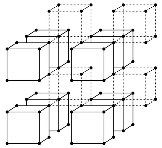
Figure 1.
Splitting the grid into cells. Cells are represented by solid lines while bonds between cells are dashed. Some dotted lines are omitted so as not to clutter up the drawing.
For the lattice having sites, (where is the number of atoms of the component i) we will have cells (where in the case under consideration).
The cells can differ in composition, and if the composition is the same, in the arrangement of the constituent atoms.
It is convenient to describe the values associated with a cell by a pair of indexes , where the first index implies that the cell has i atoms of type 1 (and, correspondingly, atoms of type 2) and the second index numbers all possible for the cell of specified composition micro-configurations:
In particular, let us denote the number of cells of type and —the internal energy of such cell (meaning the energy of bonds belonging to the cell). Then we can express the total energy E of all bonds in the system as
where is the ratio of the total count of bonds in the system to the count of bonds located inside the described ensemble of cells:
The introduced symbols can be used to express the composition of alloy:
The expression for the CF [17] is more complicated and will be constructed in several steps.
The starting point is the Bragg–Williams approximation [17] that neglects all correlations and assumes that the system allows unrestricted atom permutations:
Let us take this formula as the basic approximation. Interatomic interactions cause deviations in the distribution of atoms from a random order, and if we want to take these deviations into the account, then we must consider only the macro-configurations that are consistent with this modified distribution. Mathematically, this means that we are switching from a permutation of individual atoms to a permutation of entire cells:
We would like to treat this expression as an alternative combinatorial factor but for this purpose we must be sure that it satisfies two conditions [17]:
- –
- It achieves maximal value when atoms are distributed chaotically;
- –
- It is correctly normalized at this condition, providing the same value as Equation (5).
To be sure that the chaotic distribution in the system is achieved, we will consider the high-temperature limit, when the role of energy contribution (1) can be neglected and each lattice site is populated independently of other sites. Then:
where the superscript ∞ indicates the high-temperature limit and is the molar fraction of component j. We can now use this expression and Equations (3) and (4) to calculate the value of :
We have now shown that is an acceptable CF. We can make one step more to improve this result. Returning to Figure 1, we can say that the CF takes into account the atom correlations associated with the bonds localized inside cells. The bonds outside of cells are completely neglected. We can see also that these neglected bonds (dotted lines in the picture) form by themselves a set of cells that is in any respect similar to the original set. Naturally, we want to include correlations associated with this second cell set into the combinatorial factor.
The transition from the Bragg–Williams approximation to can be represented formally as the application of some multiplicative correction factor to :
One can say that, taking into account the bonds shown in Figure 1 by solid lines, we have reduced the CF by times. Since we have two sets of cells, we would like to accept the following expression for the CF:
where for the case under consideration.
For other grid types and with a different choice of cell size, the result may be different. In the general case, the value of can be estimated similar to the way the value was evaluated: for the case depicted in Figure 1, one set of cells is responsible for bonds belonging to this set; we need sets to ensure that all bonds are taken into account:
In our case , so we again obtain .
For the tetrahedron cell in the face-centered cubic structure .
We have now all the necessary elements to construct the expression for the free energy:
where is a temperature factor—the product of absolute temperature T and the Boltzmann constant [17]; and are the Lagrange multipliers [17].
Taking into account that
we can now obtain the basic equations of the model:
where .
The solution to these equations can be written immediately as
where are defined by
Taking into account the explicit dependency of on (5) and the expression for the free energy (12), we can now calculate the chemical potentials of components:
We must introduce some additional notation that will be required to represent all physically important objects in a compact form:
where
can be treated as the statistical sum [17] of a cell containing i atoms of type 1 and atoms of type 2.
Even if the factor in this expression is exactly equal to one, we keep it in place to have the possibility to make a more sophisticated choice of in the following sections.
Equations (3) and (4) can be rewritten now in a more compact form:
where the new notation c
was introduced to represent composition and thermodynamic activity as parametric functions of c.
First, Equation (19) defines as a function of c. Then the Equation (21) defines as a function of c. This information can be directly substituted into expressions (20) and (16) for and to complete the calculation. The necessary basis for the described calculation is the knowledge of , which are expected to be considered as the model parameters in the applications of theory.
All formulas in this section were derived in the assumption that we consider a regular lattice with a specific coordination number. However, all the details of the atom arrangements and interaction occur hidden inside the parameters . It means not only a very significant economy in the number of adjustable parameters, but also the opportunity to extend the theory outside the original assumptions. The atom distribution inside cells may be irregular but we hope that this irregularity can be encapsulated into parameters describing cells.
This consideration helps to justify the commonly-used applications of quasi-lattice approximation to liquid mixtures [3].
3. Quasichemical Theory
The Quasichemical Theory (QT) corresponds to the selection of dimers () as cells. The equations of the previous section can be applied to this case directly without any modifications. All Equations (12)–(21) remain unchanged but with a different value for . The expressions for the thermodynamic functions are presented by TISR in parametric form and we must be sure that they produce the same result as the expressions found in [16,17]. We have to remove parametric representation and convert the equations to the explicit form to confirm that the results of both theories are exactly the same. To do this, it is necessary to take into account that in the case of we have only one nontrivial (distinct from 1) value for :
since we only care about thermodynamic functions of mixing. (Here is the interaction energy of two atoms of type i and j.) It is taken into account here that and, therefore, both can be excluded from the expression for . Using these values and Equations (19) and (20) we can obtain the equation defining the parameter c:
Getting the value of c from this quadratic equation we can substitute it into the expression for the chemical potential (16), immediately reproducing the standard quasichemical expressions [16,17]:
where
The results of this section show that the simplest version of TISR ensures the precision of consideration not worse than by quasichemical theory. We can expect that the usage of cells with should improve the quality of the approximation (though usage of asymmetrical cells can diminish quality of approximation).
4. Improved Combinatorial Factor
The parameters and introduced in the Section 2 turned out to have the same value, as defined by (2) and (11). While the choice of looks quite good founded, the selection of may raise some questions. In fact, the final value of in (11) is based solely on the assumption that the distribution of bonds within one ensemble of cells is completely independent of the existence of other similar ensembles.
In classical literature devoted to QT, this type of assumption is called “non-interference hypothesis” [16]. This hypothesis looks quite plausible at high temperatures but hardly could be justified in the critical region where the correlation length aims to infinity. It can be expected that, near the critical immiscibility point, knowledge of the correlations associated with one ensemble of cells provides at least partial information about correlations associated with other ensembles. Effectively, it may mean that near the critical point the effective value of could be less than it is suggested by the “non-interference hypothesis” and defined by expression (11).
Unfortunately, there are no simple approaches to assess how the effect under discussion can affect the value of . It turns out, however, [13,14] that it is quite possible to impose an additional requirement on , which will help to ensure the reproduction of the correct critical temperature of immiscibility and at the same time significantly improve the calculated values of the most important thermodynamic quantities. This adjustment can be easily done within the framework of the Ising model—i.e., the environment that provides a comprehensive list of data related to the critical region [12] and therefore a good reference base for comparison.
The model assumes that atoms of two types are distributed over the nodes of an ideal crystal lattice and each atom interacts only with its nearest neighbors, while the interaction energy depends solely on the type of interacting atoms [12,17].
In this case the curve representing the dependency of free energy of mixing on the composition is symmetric with respect to the concentration . This behavior severely limits the direct applicability of the model to real systems, which rarely exhibit such a high level of symmetry. It means also that the immiscibility curve (binodal [2]) can be described as not trivial ) solution of the equation
Using Equation (16) for the chemical potential and definition (21) we can interpret (25) as an equation on c:
or
Assuming that is known, this transcendent equation defines c and the corresponding points on the binodal as functions of temperature . Critical point corresponds to when . Under this condition, the Equation (27) turn into an identity. Resolving this uncertainty we coming to the final expression for the critical point:
Using data from [12] and the expression (20) for , this transcendent equation can be solved for multiple two- and three-dimensional Ising models and for different approximations. The results are collected in Table 1. The table includes the most important 2D and 3D lattices and for every type of lattices several possible choices of cells are presented.

Table 1.
Critical Values (per atom) calculated using Bragg–Williams (BW), Surrounded Atom Model (SAM), Quasichemical (QT), and Improved Quasichemical Theory (IQT) [13] along with the best theoretical estimations [12].
For every type of the lattice and every cell’s size the table provides:
- –
- Size of the cell k (number of atoms included into cell);
- –
- Geometrical factor , defining location of the critical point;
- –
- Dimensionless ratio of interchange energy to the critical immiscibility temperature of alloy [9];
- –
- Dimensionless ratio of the energy per atom taken at critical temperature E to the interchange energy ;
- –
- Dimensionless expression for entropy at critical immiscibility temperature.
The column with the header BW contains critical values calculated using Bragg–Williams approximation.
The column with the header QT contains critical values calculated using Quasichemical Theory.
The column with the header SAM contains critical values calculated using Surrounded Atom Model. Even if the cell size used by SAM is larger than the size of the quasichemical cell (equal two), it is evident from the table, that SAM provides precision significantly worse than standard QT. This error introduced by standard Surrounded Atom Model will be explained and corrected in the Section 5.
The column with the header IQT corresponds to the Improved Quasichemical Theory—i.e., Quasichemical Theory where parameter of model is adjusted to reproduce the correct critical temperature, as explained above. Comparison of column QT and IQT shows that adjustment of critical temperature significantly improves quality of approximation.
Even better results can be found in the IQT2 column, which considers cells that better match the geometrical structure of the simulated grids. Accordingly, the following choices are made:
- –
- for a square lattice, a regular square (k = 4) is a natural choice;
- –
- for a triangular lattice, a regular triangle (k = 3) is the choice;
- –
- for a simple cubical lattice, a regular cube (k = 8) is the choice;
- –
- for a Body Centered Cubical (BCC) lattice, an irregular tetrahedron (k = 4) with two vertices in the main grid and two vertices from the sublattice formed by central atoms;
- –
- for a Face Centered Cubic (FCC) lattice, a regular tetrahedral (k = 4) is the choice.
In general, the data in the table show that the “Improved Quasichemical Theory” (IQT and IQT2) really provides significant improvements compared to the standard Quasichemical Theory (QT).
The possibility to completely eliminate the error in determining the location of the critical point in the phase diagram should be considered extremely important if one remembers that the usual quasichemical 10% shift in the critical temperature value can mean a defect up to (or even more) for typical metal alloys. Data in the table show also that the adjustment of the critical temperatures helps at the same time to reduce significantly the errors in estimating the critical values of energy and entropy of the alloy. This fact can be confirmed and clarified by Figure 2, which shows two different versions of the CF at , compared to the exact CF derived by [18] using the Onsager solution [19] for the square lattice.
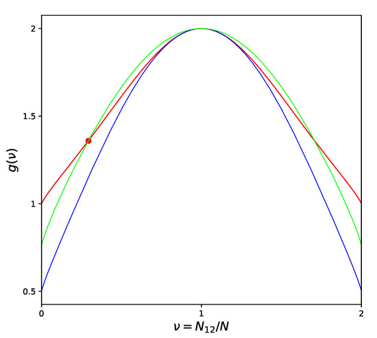
Figure 2.
Different Approximations of the Combinatorial Factor for a Square lattice: Quasichemical approximation—blue line; Improved Quasichemical approximation—green line; Onsager solution [19]—red line; Location of the critical point by [19]—large dot.
High temperature corresponds to chaotic atom distribution (equivalent to for the square lattice) and we can see from the picture that in this region the ordinary QT approximation is extremely close to the Onsager’s solution. When the temperature decreases and we approach the critical point, then the difference between QT and the exact curve sharply increases. On the contrary, partially losing the quality of approximation in the high-temperature limit, IQT provides a more uniform (though hardly perfect) representation of the exact curve over the entire range from high temperatures to the critical point. Exaggerating, we can say that QT is very good around one point, while IQT is reasonably good inside the whole physically meaning region. This is the real reason why all the related values improve when we switch from QT to IQT.
In the above part of this section, we considered the systems with positive deviation from Raoult’s Law [7] only. The atoms in these systems prefer to be surrounded by atoms of the same type, especially when the temperature drops and approaches the critical point. Atoms in systems with negative deviations from Raoult’s law tend to be surrounded by atoms of the opposite kind, but this tendency can be severely limited in some cases. The Face Centered Cubic lattice is the most important example. No matter how one divides the lattice into two sublattices, each atom will have neighbors from both sublattices. As result, some part of the bonds will be of or type and the proportion of pairs can never exceed 2/3, as seen from Figure 3.
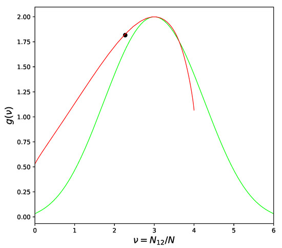
Figure 3.
Versions of Combinatorial Factor for FCC Lattice: Quasichemical approximation—green line; Improved Quasichemical approximation with —red line; Location of the critical point by [12]—large dot.
Such condition is commonly known as “geometrical frustration” [20]. Frustration-free lattices, such as Cubical or Body Centered Cubical, have an additional symmetry [17], which effectively leads to a symmetric form of CF dependence on the number of pairs , as in Figure 2. Frustrated lattices are critically different in this respect but the asymmetrical behavior of CF cannot be recognized on the level of pair-like approximation. We need four or more atoms to be included in the cell in order to correctly represent the three-dimensional structure of the alloy and to be sure that the frustration phenomenon is described correctly.
Returning to Figure 3 we can see that the left branch of CF curve goes above the quasichemical graph. The value of corresponding to the left branch is less than the quasichemical value, in agreement with the heuristic arguments at the beginning of the section. The ordering phase transition in the FCC lattice (right branch) is of the first order [10] and therefore these arguments cannot be applied. Indeed, as can be seen from Figure 3 and will be confirmed in the Section 7, the ordering in the Au − Cu system has to be described by which is larger than the quasichemical estimation (11).
5. Surrounded Atom Model
The Surrounded Atom Model (SAM) was introduced in [21,22] as a direct generalization of quasichemical theory. The motivation for such generalization was the well-known deficiency of QT [16] which is not capable to describe systems with any asymmetry on the curve representing the dependence of thermodynamic values on the composition. The generalization was achieved by replacing the dimers, used as the basis of QT, by groups of atoms, where every group consists of one “central” atom and all z its nearest neighbors. This approach opens the possibility to introduce the direct dependence of atom interactions on the local composition and explain in this way the asymmetry, if any. Though SAM cannot be considered as popular as QT, it is still in use [23,24,25,26] because of its intuitive appeal.
The formalism of theory was constructed to mimic the arguments used by [16] to derive the classical QT equations, but a sad mistake in the calculation of the CF—the basic element of theory—significantly impaired the quality of the resulting model.
To describe the “surrounded atoms” in the framework of TISR, we selecting as a cell the same configuration as SAM does: atom surrounded by z nearest neighbors. Just as is commonly accepted by SAM, only z bonds between the central atom and the shell are included in the cell; bonds between the surrounding atoms are excluded. A central atom in the cell occurs in a special position and we must take extra care to be sure that central and peripheral atoms have the same average composition. To handle this task, we can present a cell as a combination of two sub-cells, where the central atom constitutes one sub-cell, while z surrounding atoms are included in other sub-cell.
It is convenient for the following calculations to define the sub-cell that contains z peripheral atoms as the first sublattice (). The central atom is then the only element of the second sub-cell (). Thus, the total size of the cell is
To completely describe a cell we must specify the content of every sub-cell and indicate how atoms are distributed. To do this we will need three indexes, and in the remainder of this section will mean the number of cells having every:
i atoms of type a in sub-cell 1;
j atoms of type a in sub-cell 2;
will number all possible configurations of a cell having i atoms of type a in sub-cell 1 and j such atoms in sub-cell 2:
The CF will be still expressed by Equation (10) where is defined this time as
Taking into account the existence of sub-cells, we can write down the free energy of the system in the following form:
where we have additional (compared to (12)) restriction included and
The structural parameter , when taken in the quasichemical approximation, is equal to
As immediately follows from the expression (32) for the free energy,
So far, we have not imposed any restrictions on the dependence of cell’ energy on the composition, that is so important in SAM. But since our primary interest is the behavior of CF, from this moment on we will assume that the energy of cells follows strongly the simple rules of the Ising model [2]:
where, as in (22)
This assumption cannot influence the CF, which depends on the geometrical structure of the lattice only, but significantly simplifies and clarifies our work by reducing both models to the ordinary quasichemical theory (some simplification that is certainly impossible in the general case when the energy of the “surrounded atom” is an arbitrary functional of the composition).
As the result of the assumption (38), and as it follows from (35), we can see immediately that the probabilities are independent of , so we can introduce new variables :
where, in agreement with the usual SAM notation [21,22]:
In general, the notations used by SAM and TISR differ significantly and should be brought to a common basis for comparison. In particular, the ensemble of “surrounded atoms” consists of N elements, while the TISR’ ensemble includes only elements. This difference has to be taken in the account when comparing the intermediate values. The variables describing cells are defined differently inside SAM [27], where denotes the number of atoms a surrounded by i atoms b, and denotes the number of atoms b surrounded by i atoms a:
The critical point, where the difference between TISR and SAM becomes evident, is the expression for the CF, namely, the part of the expression for the free energy (32) that includes :
This expression contains an extra multiplier , compared to [27]. The same problem can be indicated in the expression for the internal energy of the system:
Again, we have here extra factor that is missing in SAM [27]. It means that the equations of SAM can be formally received from the equations of TISR if we replace the common value of by the value that is two times larger.
The source of this difference is easy to understand. Parameters and are defined above by conditions (2) and (11), which are actually identical, so we will consider as an example the second equation only:
We can say that is selected to ensure that every bond in the system is counted in the CF precisely one time.
CF in SAM is constructed [27,28] by treating the “surrounded atoms” as independent entities, rather than pairs. It looks natural but it is the source of the problem. Let us consider an arbitrary pair of neighboring atoms . We can identify the “surrounded atom” where m is the central atom and is located in its shell. We can consider also the “surrounded atom” where is the central atom and m is located in its shell. But it means that when calculating the CF, the pair is taken into account twice, while in TISR, as we have seen, every pair is taken into account only once.
As result, the accuracy of SAM is only intermediate between the accuracy of the Bragg–Williams approximation and the accuracy of the quasichemical theory, as can be seen from Table 1. At the same time, the fixed here version of TISR ensures a quasichemical level of precision. And it can be significantly improved by refining the CF of the system as shown in Section 4.
6. Associated Solution Model
Detailed description of ASM is given in [15]. It contains a complete resolution of multiple problems that this model has been suffering from for many years [3,7,8,29]. Here we indicate only the main problems referring to [15] for details.
Using the Equation (17) that defines the probability to find a cell of given composition, we can construct an expression that contains no parameters at all and therefore is a function of the temperature only:
It looks precisely as the mass action equation for the ideal Association Solution Model (ASM) ([30]), where cells are treated as “associates”. In this sense we can say that TISR is always formally equivalent to some effective ideal ASM but includes several significant differences.
First, we can see that the expression (1) for the energy of alloy can be divided in two parts:
where the first term can be treated as formation energy of cells that are treated as “associates”. The second term has to be considered therefore as interaction energy of “associates”.
Second, the Equation (45) includes “associates” of all possible compositions—this never happens in common ASM. This fact is critically important to resolve the well known high-temperature anomalies of ASM [15].
The difference between the two theories will become even clearer if we take into account the specifics of the choice of the CF. The standard for ASM selection of CF is based on the Bragg–Williams approximation [17] being applied to associates, and can be formally derived from the TISR expression (10) at . If we return to the Equation (28) describing the critical point, we can see that is the point of singularity at which this equation has no solution.
This remark confirms the good know fact that the ideal ASM is not capable to describe the systems with positive deviations from Raoult’s Law [29].
At the same time, it can be shown [15] that the efficient TISR-based ASM corresponds to and is completely free of this and many other problems that are so typical for standard ASM [3,7,8,29].
The discussed above possibility to rewrite the equations of TISR in the form similar to the equations of ideal ASM opens the possibility to immediately use TISR for phase diagram calculations since most of the existing phase diagram calculation engines implement ASM. However, this issue is beyond the scope of this article.
Directly related to all mentioned questions is the physical interpretation of ASM equations, which has been discussed in detail in [15].
7. Order–Disorder Transformations
All systems considered in the previous sections show positive deviations from ideality. At low temperatures they usually trend to split in several phases of distinct composition. In this section we will consider crystalline systems providing negative deviations from ideality.
As is well known [7], at low temperatures, atoms in such systems can be redistributed over several intertwined sublattices with the formation of phases usually identified as superalloys [7,8]. Such systems were considered in classical papers devoted to the quasichemical theory [31,32,33] and later the developed approach was improved in a number of papers related to “cluster-site approximation” [34,35]. We will show how the standard approach developed in the current article precisely reproduces the results of the described models.
As could be expected, mathematical description requires some specific in this case. As a working example, we will consider the superstructure Cu3Au, which appears in the Cu–Au system below a certain critical temperature and has an FCC lattice [2]. It is also well known that the Cu3Au superstructure can be represented as the union of two intertwined sublattices, one of which is preferable for Cu and has three times as many nodes as the second sublattice, preferable for Au. It is convenient for our consideration to distinguish these sublattices by an index (which, we assume, varies from one to two). Naturally, in our case, the selection of a tetrahedron as the basic cell results in identifying two sub-cells inside every cell. One of the sub-cells has three nodes and is preferable for Cu, while the second sub-cell has one node and is preferable for Au. We assign an index to every sub-cell to be identical with the index of the corresponding sublattice.
The configuration of the system can be described now as follows.
The lattice having knots is divided into cells containing every knots. We need two variables to specify the count of knots in each sub-cell:
It means that the total number of knots in the sublattice m is
To describe a cell we must specify the content of every sub-cell. We will use for this purpose two indexes .
Accordingly, is the number of cells having every:
i atoms of type a in sub-cell 1;
j atoms of type a in sub-cell 2;
index identifies one of the configurations possible for the cell of specified composition:
In the following part of this section, the superscript indicates the sublattice, while the subscript is the component’s number. In particular, the total number of atoms a belonging to the sublattice m is:
with the total number of atoms a in the system:
The concentration of atoms a (calculated for every sublattice separately) is:
where
The previously introduced local per-sublattice concentrations are directly related to the total alloy composition:
The structural parameter , considered in the quasichemical approximation (11), turns out to be equal to 4. The energy of the entire system is
and differs from the expression (1) only by using two indexes required to specify the cell composition. The configurational entropy of the system reaches its maximum when both sublattices have the same composition. The order–disorder transition occurs when the interatomic interaction is strong enough to spontaneously destroy the equality of atomic concentrations. Accordingly, the variables obtain dynamically-defined values (that can still be uniquely expressed by the formula (51)). The free energy of the system can be written now as a natural generalization of (12):
The basic equations of theory can be obtained by minimization of F with respect to :
The first of these equations can be immediately solved in a usual form:
where b and are defined through
As always, we introduce now a few additional variables that help to present the equilibrium equations in a traceable form:
where
so the Equations (51) and (52) can be rewritten as:
where
To simplify the derived equations we substitute the expressions for given by (63) into the Equation (53):
This equation has to be combined with the normalization condition (64) to remove b.
The expression for will look simpler if we define a few more combinations:
Finally,
Expressing from this equation we will have a solution where defines distribution of components between sublattices, while ensures the correct total composition of the system. Equation (58) (with all components expressed as functions of ) defines the values of that bring the extreme values to the free energy.
Returning to the expression (56), we can simplify it using the equation of equilibrium (57). As a result, all components linear in will be canceled:
and all dynamic variables on the right side are assumed now to be expressed through using (60) and (63).
Now it turns out that the expression for free energy (68) is identical to the corresponding expression from [34] (Equation (5)). This becomes apparent if one uses the correspondence list between the notations used in the current article and the notations introduced by [34] presented in Table 2.
Table 2.
Notation correspondence between [34] and the current article.
Proposed in [34], modifications to CSA were necessary to reproduce the results of the Monte Carlo experiments [36] and occurred very successfully. It happen to be the same modifications that were independently introduced by TISR many years ago [13,14] and described in Section 4. Based on this coincidence, we can now take the value of found by Oates and substitute it into the equations of the current chapter.
The remaining equation could be solved numerically, but it is more instructive to look at the plot of the free energy of the system versus the concentration of atoms a in the first sublattice. Drawing this plot is an easy task taking into account the described above dependency of both values on as a parameter (Figure 4).
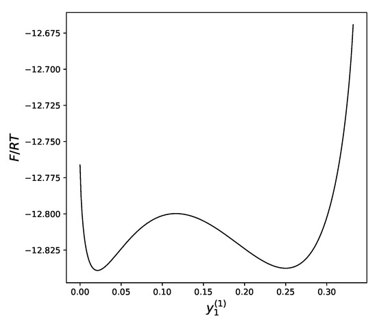
Figure 4.
Molar free energy of alloy near the critical point as a function of the concentration of atoms a in the first sublattice: and .
We can see that at sufficiently low temperatures, the dependency of the free energy on the distribution of atoms between the sublattices has two local minima: one that corresponds to a uniform distribution of atoms over all sublattices (near ), and another, which demonstrates a significant difference in the concentration of atoms between the two sublattices.
The temperature is the main factor that defines which of these two minima will win the competition, bringing, therefore, the lowest value to the free energy.
8. Multicomponent Systems
The multicomponent generalization of thermodynamic models is an important task that can cause significant mathematical difficulties that usually increase with the number of components. For example, we discussed in Section 3 the explicit solution (24) found for the quasichemical model in a two-component system. Generalization of this model, even for ternary alloys, produces a system of nonlinear equations that only allow a numerical solution [37].
The same problem exists in the case of multicomponent ASM [38], where even the binary system formalism cannot avoid using nonlinear equations. The multicomponent generalization of ASM encounters even more principal difficulties when attempting to define multicomponent associates and the interaction between them [8].
In contrast, the parametric representation of a solution using TISR makes multicomponent generalization almost trivial in most cases. Usually, it only requires the replacement of the index i, which describes the cell composition in the binary system, by a n-component vector:
where
As result, we have the following expression for the energy:
where
The composition of the alloy is then
CF is still expressed by (10) where this time
and
appear as direct generalization of expressions (5) and (6). Free energy can be written as:
Omitting the standard steps, we obtain:
while the expression for the chemical potential (16) remains unchanged.
Thanks to the condition (69), all the physically meaningful values depend effectively on independent variables, ensuring the parametric presentation of properties.
This short review makes the details of multicomponent generalization totally clear in the case when all knots inside a cell are equivalent. If a cell has to be divided into two (or more) sub-cells (as happen in the case of the Surrounded Atom Model, Section 5), we need more than one vector index to describe such cell. The key Equation (61) is presented now as
The presence of two vector variables leads to more cumbersome equations; however, the main logic remains unchanged.
9. Results and Disscussion
Combining several model theories within a general scheme is a complex and important problem. This article attempts to achieve this goal by presenting the CF of the theory in a new form that is more intuitive, more general, and allows more precise control over accuracy than traditionally-used constructs. The developed approach allows for the first time utilization of the same formalism to reproduce the results of several theories, including Quasichemical Theory, Associated solution model, Surrounded Atom Model, and Cluster Site Approximation. It is shown that by simply choosing a specific group of atoms—cells—for each model one can reproduce—or even significantly improve—the results of the above theories.
Remarkably, in all cases, the expressions for the energy and for the CF remain basically the same. What changes is the set of indexes necessary to identify the composition and structure of each cell, and the set of external constraints that must be added to the free energy functional to fix the total composition and (in some cases) ensure the internal consistency of the formalism.
An unusual feature of the theory is the presentation of the results in a parametric form, where both the thermodynamic quantities and the concentrations of the components are expressed as functions of a common parameter (or several parameters, in the case of a multicomponent system) that naturally arise as part of the solution. Surprisingly, it is the use of this parametric form that drastically simplifies formalism, especially multicomponent generalizations of the theory.
The combinatorial factor developed within the framework of the theory has proved its advantages, helping to find and correct some errors found in the associated solution model and in the surrounded atom model. The identified errors, if left uncorrected, could jeopardize the accuracy and physical interpretation of these theories. Moreover, the new CF, which without any tricks ensures the accuracy of calculations at the level of quasichemical theory, also allows some modifications that ensure the reproduction of the correct critical temperature of the alloy and significantly increases the accuracy of all thermodynamic quantities.
In general, the presented approach allows us to obtain the following new results:
- –
- A new formalism, equally applicable to several independent models;
- –
- Identification and correction of serious errors in ASM and SAM;
- –
- An extended version of the formalism that allows the recreation of the correct critical temperature and significantly improves the accuracy of calculations for QT, ASM, and SAM.
Finally, very important for the potential application of TISR, is the drastic reduction in the number of adjustable parameters needed to describe the thermodynamic properties of alloys. For example, when considering the FCC lattice in the tetrahedral approximation, we need:
- –
- Three temperature-dependent parameters to describe a binary system;
- –
- Three additional temperature-dependent parameters to describe the comprising ternary system;
- –
- One additional temperature-dependent parameter to describe the containing quaternary system;
- –
- No additional parameters for the systems with five or more components.
We can expect that the possibility of applying this economic approach to a wide range of systems creates a large space for potential applications of theory.
10. Applications of TISR
This section presents the application of TISR formalism to several binary systems known from the literature. The purpose is to demonstrate the possibilities of TISR for describing various in strength metallic binary systems using the minimal tetrahedral approximation. This approximation uses three temperature-dependent parameters to describe integral enthalpy of mixing and activities of components. In all considered cases the polynomial description of thermodynamic functions were taken from the open publications and used as input. Based on this input, the adjustable TISR parameters were obtained using linear regression analysis.
In all the figures below (Table 3), the original data from the literature are shown by solid lines. TISR calculations were performed in the tetrahedral approximation and the results are presented by the dotted lines. The summary of results is available in the table below (where is abbreviated as for compactness).
Table 3.
TISR parameters adjusted to the input polynomials taken from the literature.
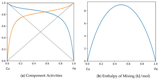
Figure 16.
System Cu-Fe (T = 1873 K): solid lines—[49]; dotted lines—TISR.
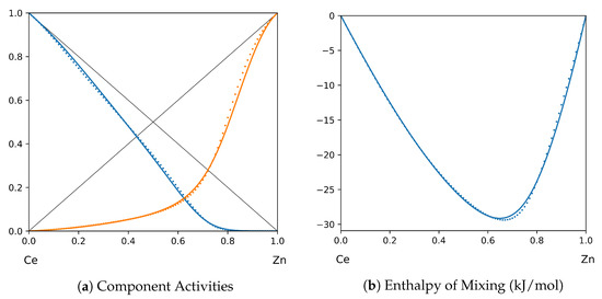
Figure 15.
System Ce-Zn (T = 1873 K): solid lines—[48]; dotted lines—TISR.
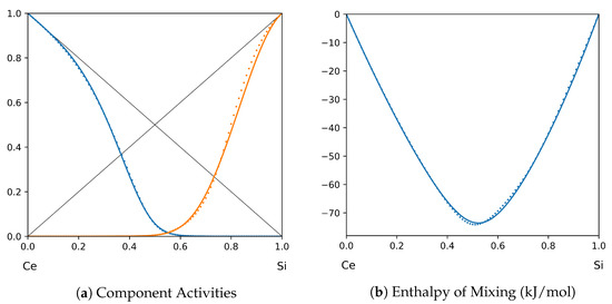
Figure 14.
System Ce-Si (T = 1923 K): solid lines—[47]; dotted lines—TISR.
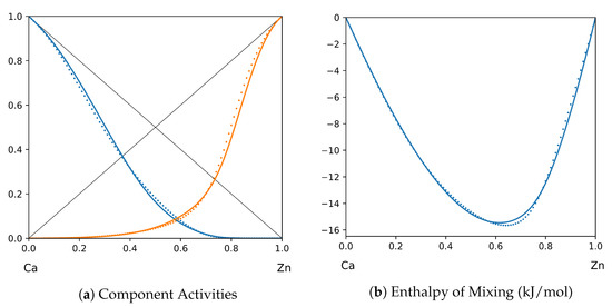
Figure 13.
System Ca-Zn (T = 1520 K): solid lines—[46]; dotted lines—TISR.
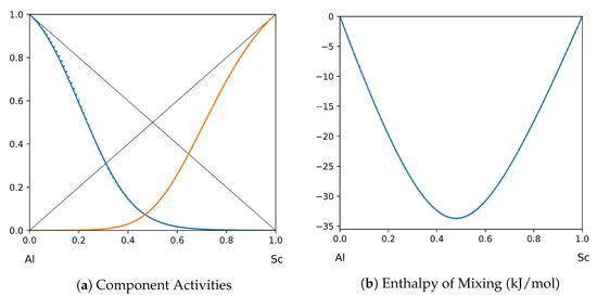
Figure 12.
System Al-Sc (T = 1873 K): solid lines—[45]; dotted lines—TISR.
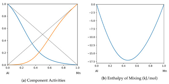
Figure 11.
System Al-Mn (T = 1520 K): solid lines—[44]; dotted lines—TISR.
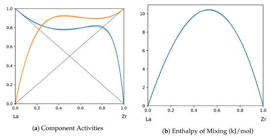
Figure 10.
System La-Zr (T = 1800 K): solid lines—[43]; dotted lines—TISR.
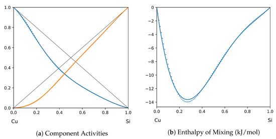
Figure 9.
System Cu-Si (T = 1575 K): solid lines—[41]; dotted lines—TISR.
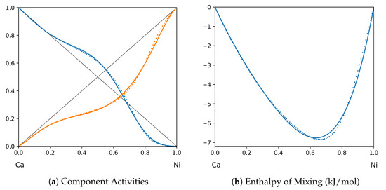
Figure 8.
System Ca-Ni (T = 1120 K): solid lines—[42]; dotted lines—TISR.
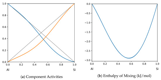
Figure 7.
System Al-Si (T = 1575 K): solid lines—[41]; dotted lines—TISR.
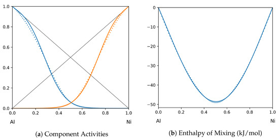
Figure 6.
System Al-Ni (T = 1923 K): solid lines—[40]; dotted lines—TISR.
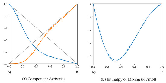
Figure 5.
System Ag-In (T = 1200 K): solid lines—[39]; dotted lines—TISR.
Funding
This research received no external funding.
Data Availability Statement
Not applicable.
Conflicts of Interest
The authors declare no conflict of interest.
Abbreviations
The following abbreviations are used in this manuscript:
| ASM | Association Solution Model |
| BW | Bragg–Williams approximation |
| CEF | Compound Energy Formalism |
| CF | Combinatorial Factor |
| CSA | Cluster Site Approximation |
| CVM | Cluster Variation Method |
| FCC | Face Centered Cubic lattice |
| IQT | Improved Quasichemical Theory |
| LRO | Long-Range Order |
| QT | Quasichemical Theory |
| SRO | Short-Range Order |
| SAM | Surrounded Atom Model |
| TISR | Theory of Inhomogeneous Short-Range Order |
References
- Morán-López, J.L.; Sánchez, J.M. (Eds.) Theory and Applications of the Cluster Variation and Path Probability Methods; Springer Science & Business Media: New York, NY, USA, 2012. [Google Scholar]
- Girifalco, L.A. Statistical Mechanics of Solids; Oxford University Press: Oxford, UK, 2000. [Google Scholar]
- Soustelle, M. Modeling of Liquid Phases (Chemical Thermodynamics Set); Wiley-ISTE: London, UK, 2015. [Google Scholar]
- Lupis, C.H.P. Chemical Thermodynamics of Materials; Prentice Hall: Englewood Cliffs, NJ, USA, 1983. [Google Scholar]
- Oates, W.; Wenzl, H. The cluster/site approximation for multicomponent solutions—A practical alternative to the cluster variation method. Scr. Mater. 1996, 35, 623–627. [Google Scholar] [CrossRef]
- Ossi, P. Disordered Materials: An Introduction; Springer Science & Business Media: New York, NY, USA, 2010. [Google Scholar]
- Lukas, H. Computational Thermodynamics: The Calphad Method; Cambridge University Press: Cambridge, MA, USA, 2007. [Google Scholar]
- Sundman, B.; Chen, Q.; Du, Y. A Review of Calphad Modeling of Ordered Phases. J. Phase Equilibria Diffus. 2018, 39, 678–693. [Google Scholar] [CrossRef]
- Gusev, A.I.; Rempel, A.A.; Magerl, A.J. Disorder and Order in Strongly Nonstoichiometric Compounds; Springer: Berlin/Heidelberg, Germany, 2001. [Google Scholar]
- Krivoglaz, M.; Smirnov, A. The Theory of Order-Disorder in Alloys [Translated from the Original Russian by Scripta Technica. Edited by Bruce Chalmers]; Macdonald: London, UK, 1964. [Google Scholar]
- Christian, J.W. The Theory of Transformations in Metals and Alloys; Newnes: Newton, MA, USA, 2002. [Google Scholar]
- Domb, C. Ising Model. In Phase Transitions and Critical Phenomena, Volume 3; Academic Press: New York, NY, USA, 1974; pp. 357–485. [Google Scholar]
- Vajsburd, S.; Kremer, E. An improved quasi-chemical method and mathematical aspects of its use in the thermodynamics of solutions with an arbitrary number of components (In Russian). In Mathematical Problems of Chemical Thermodynamics; Kokovin, G., Ed.; Nauka: Novosibirsk, Russia, 1985; pp. 89–96. [Google Scholar]
- Kremer, E. Theory of Inhomogeneous Short Range Order and its Usage for Description the Thermodynamic Properties of Sulfide Melts of Iron, Cobalt, and Nickel (In Russian). Ph.D. Thesis, Leningrad State University, Leningrad, Russia, 1988. [Google Scholar]
- Kremer, E. Associated solution model rebuilt. Calphad 2022, 77, 102408. [Google Scholar] [CrossRef]
- Guggenheim, E. Mixtures; Oxford University Press: Oxford, UK, 1952. [Google Scholar]
- Hill, T.L. Statistical Mechanics; McGraw-Hill Book Company, Inc.: New York, NY, USA, 1956. [Google Scholar]
- Prigogine, I.; Mathot-Sarolea, L.; Hove, L.V. On the combinatory factor in regular assemblies. Trans. Faraday Soc. 1952, 48, 485. [Google Scholar] [CrossRef]
- Onsager, L. Crystal Statistics. I. A Two-Dimensional Model with an Order-Disorder Transition. Phys. Rev. 1944, 65, 117–149. [Google Scholar] [CrossRef]
- Sadoc, J.F. Geometrical Frustration; Cambridge University Press: Cambridge, MA, USA, 1999. [Google Scholar]
- Mathieu, J.C.; Durand, F.; Bonnier, É. L’atome entouré, entité de base d’un modèle quasichimique de solution binaire. J. Chim. Phys. 1965, 62, 1289–1296. [Google Scholar] [CrossRef]
- Hicter, P.; Mathieu, J.; Durand, F.; Bonnier, E. A model for the analysis of enthalpies and entropies of liquid binary alloys. Adv. Phys. 1967, 16, 523–533. [Google Scholar] [CrossRef]
- Lehmann, J. Application of ArcelorMittal Maizières thermodynamic models to liquid steel elaboration. Rev. Métallurgie 2008, 105, 539–550. [Google Scholar] [CrossRef]
- Lehmann, J.; Zhang, L. The Generalized Central Atom for Metallurgical Slags and High Alloyed Steel Grades. Steel Res. Int. 2010, 81, 875–879. [Google Scholar] [CrossRef]
- Ha, D.C.; Khanh, N.N. The Surrounded Atom Theory of Order-disorder Phase Transition in Binary Alloys. Commun. Phys. 2011, 21, 265. [Google Scholar] [CrossRef]
- Kotova, N.; Golovata, N.; Usenko, N. Calculation of thermodynamic properties of liquid Fe-Ln alloys. Fr.-Ukr. J. Chem. 2015, 3, 40–43. [Google Scholar] [CrossRef]
- Kapoor, M.L. An Approach to Thermodynamics of Binary Substitutional Solutions. Trans. Jpn. Inst. Met. 1978, 19, 519–529. [Google Scholar] [CrossRef][Green Version]
- Bichara, C.; Bergman, C.; Mathieu, J.C. Monte Carlo calculations of thermodynamic properties of alloys in the case of the surrounded atom model. Acta Metall. 1985, 33, 91–95. [Google Scholar] [CrossRef]
- Pelton, A.D.; Kang, Y.B. Modeling Short-Range Ordering in Solutions. Int. J. Mater. Res. 2007, 98, 907–917. [Google Scholar] [CrossRef]
- Schmid, R.; Chang, Y.A. A thermodynamic study on an associated solution model for liquid alloys. Calphad 1985, 9, 363–382. [Google Scholar] [CrossRef]
- Yang, C.N. A Generalization of the Quasi-Chemical Method in the Statistical Theory of Superlattices. J. Chem. Phys. 1945, 13, 66–76. [Google Scholar] [CrossRef]
- Yang, C.N.; Li, Y. General Theory of the Quasi-Chemical Method in the Statistical Theory of Superlattices. Chin. J. Phys. 1947, 11, 59–71. [Google Scholar]
- Li, Y.Y. Quasi-Chemical Theory of Order for the Copper Gold Alloy System. J. Chem. Phys. 1949, 17, 447–454. [Google Scholar]
- Oates, W.A.; Zhang, F.; Chen, S.L.; Chang, Y.A. Improved cluster-site approximation for the entropy of mixing in multicomponent solid solutions. Phys. Rev. B 1999, 59, 11221–11225. [Google Scholar]
- Oates, W. Configurational entropies of mixing in solid alloys. J. Phase Equilibria Diffus. 2007, 28, 79–89. [Google Scholar] [CrossRef]
- Ferreira, L.G.; Wolverton, C.; Zunger, A. Evaluating and improving the cluster variation method entropy functional for Ising alloys. J. Chem. Phys. 1998, 108, 2912–2918. [Google Scholar] [CrossRef]
- Mickeleit, M.; Lacmann, R. Statistical mechanics and thermodynamic properties of liquid multicomponent mixtures. Part I. The Taylor series for quasichemical equilibrium of ternary mixtures. Fluid Phase Equilibria 1983, 12, 201–216. [Google Scholar] [CrossRef]
- Pok-Kai, L.; Ching-Hua, S.; Tse, T.; Brebrick, R. Quantitative simultaneous fit to the liquidus surface and thermodynamic data for the Ga-In-Sb system using an associated solution model for the liquid. Calphad 1982, 6, 141–169. [Google Scholar] [CrossRef]
- Zivkovic, D.; Manasijevic, D.; Mihajlovic, I. Calculation of the thermodynamic properties of liquid Ag–In–Sb alloys. J. Serb. Chem. Soc. 2006, 71, 203–211. [Google Scholar] [CrossRef]
- Huang, W.; Chang, Y. A thermodynamic analysis of the Ni–Al system. Intermetallics 1998, 6, 487–498. [Google Scholar] [CrossRef]
- He, C.Y.; Du, Y.; Chen, H.L.; Xu, H. Experimental investigation and thermodynamic modeling of the Al–Cu–Si system. Calphad 2009, 33, 200–210. [Google Scholar] [CrossRef]
- Uremovich, D.; Islam, F.; Medraj, M. Thermodynamic modeling of the Ca–Ni system. Sci. Technol. Adv. Mater. 2006, 7, 119–126. [Google Scholar] [CrossRef]
- Mattern, N.; Yokoyama, Y.; Mizuno, A.; Han, J.; Fabrichnaya, O.; Richter, M.; Kohara, S. Experimental and thermodynamic assessment of the La-Ti and La-Zr systems. Calphad 2016, 52, 8–20. [Google Scholar] [CrossRef]
- Shukla, A.; Pelton, A.D. Thermodynamic Assessment of the Al–Mn and Mg–Al–Mn Systems. J. Phase Equilibria Diffus. 2008, 30, 28–39. [Google Scholar] [CrossRef]
- Kang, Y.B.; Pelton, A.D.; Chartrand, P.; Fuerst, C.D. Critical evaluation and thermodynamic optimization of the Al–Ce, Al–Y, Al–Sc and Mg–Sc binary systems. Calphad 2008, 32, 413–422. [Google Scholar] [CrossRef]
- Wasiur-Rahman, S.; Medraj, M. Critical assessment and thermodynamic modeling of the binary Mg–Zn, Ca–Zn and ternary Mg–Ca–Zn systems. Intermetallics 2009, 17, 847–864. [Google Scholar] [CrossRef]
- Shukla, A.; Kang, Y.B.; Pelton, A.D. Thermodynamic assessment of the Ce–Si, Y–Si, Mg–Ce–Si and Mg–Y–Si systems. Int. J. Mater. Res. 2009, 100, 208–217. [Google Scholar] [CrossRef]
- Zhu, Z.; Pelton, A.D. Critical assessment and optimization of phase diagrams and thermodynamic properties of RE–Zn systems-part I: Sc–Zn, La–Zn, Ce–Zn, Pr–Zn, Nd–Zn, Pm–Zn and Sm–Zn. J. Alloys Compd. 2015, 641, 249–260. [Google Scholar] [CrossRef]
- Shubhank, K.; Kang, Y.B. Critical evaluation and thermodynamic optimization of Fe–Cu, Cu–C, Fe–C binary systems and Fe–Cu–C ternary system. Calphad 2014, 45, 127–137. [Google Scholar] [CrossRef]


Disclaimer/Publisher’s Note: The statements, opinions and data contained in all publications are solely those of the individual author(s) and contributor(s) and not of MDPI and/or the editor(s). MDPI and/or the editor(s) disclaim responsibility for any injury to people or property resulting from any ideas, methods, instructions or products referred to in the content. |
© 2023 by the author. Licensee MDPI, Basel, Switzerland. This article is an open access article distributed under the terms and conditions of the Creative Commons Attribution (CC BY) license (https://creativecommons.org/licenses/by/4.0/).