Spatial Bias in Open Biodiversity Data: How GBIF Record Quality Shapes Conservation Analyses

Abstract

Open-access biodiversity repositories such as the Global Biodiversity Information Facility (GBIF) are central to contemporary conservation research, yet their heterogeneous data sources introduce quality issues and spatial sampling biases that may compromise conservation analyses. This study evaluates the spatial and taxonomic quality of GBIF occurrence data for five protected species representing mammals and vascular plants in Central Europe. A transparent data-cleaning workflow was applied, including coordinate validation, removal of duplicate and erroneous locations, and taxonomic harmonization. Spatial sampling bias was quantified using nearest neighbor distance-based metrics, enabling comparison of clustering patterns before and after data cleaning. Raw datasets exhibited strong spatial clustering across all species, with nearest neighbor ratios (NNR) ranging from 0.06 to 0.73. Data cleaning reduced the number of retained records by approximately 15–57% and increased NNR values to 0.27–0.80, indicating the removal of extreme spatial artifacts. However, NNR values remained well below unity after cleaning, demonstrating persistent non-random spatial sampling structure related to uneven sampling effort. The strongest relative improvements were observed for plant species derived from herbarium records. These results highlight the need to distinguish between data quality errors and structural spatial bias in open biodiversity data and underscore the necessity of bias-aware methods beyond standard data-cleaning procedures in conservation analyses.

1. Introduction

Reliable information on species distributions is a cornerstone of effective conservation planning, biodiversity monitoring, and ecological decision-making [1,2,3]. Spatially explicit occurrence data underpins a wide range of conservation applications, including biodiversity assessments, reserve design, connectivity analyses, and evaluations of environmental change [1,4]. In recent years, the rapid growth of open-access biodiversity repositories has profoundly transformed conservation science by enabling large-scale analyses [5,6,7].

Among these repositories, the Global Biodiversity Information Facility (GBIF) has become one of the most comprehensive global platforms for biodiversity occurrence data, integrating records from museums, herbaria, monitoring programs, and citizen science initiatives [8,9,10,11,12]. GBIF data are now widely used in conservation-oriented analyses and spatial assessments, providing opportunities for transparent and reproducible research. At the same time, the heterogeneous origin of this data introduces important challenges related to data quality and representativeness [13,14,15].

Occurrence records derived from open biodiversity databases may suffer from multiple sources of error and uncertainty. Common issues include spatial inaccuracies caused by coordinate rounding, assignment to administrative centroids or institutional locations, and the retrospective georeferencing of imprecise locality descriptions. In addition, taxonomic inconsistencies arising from synonymy, outdated nomenclature, or misidentifications remain a persistent concern, especially in historical and herbarium-based datasets [13,15,16].

Sampling effort in open biodiversity databases is rarely evenly distributed, with occurrence records typically clustered near accessible areas such as roads, urban centers, protected sites, or research institutions. While citizen science initiatives have substantially increased data availability, they may also intensify accessibility-driven bias. If unrecognized or unquantified, such biases can distort spatial analyses and lead to misleading inferences about species distributions and conservation priorities [13,17,18].

Importantly, the nature and magnitude of data quality issues and spatial bias differ among taxonomic groups [15,19,20]. Occurrence data for animals, particularly large or conspicuous species, are often dominated by opportunistic observations and citizen science contributions, resulting in pronounced spatial clustering [21,22]. In contrast, plant occurrence data frequently originate from herbarium collections and historical surveys, where spatial precision and temporal resolution may vary substantially, and multiple records may be associated with identical or near-identical localities [23,24].

Despite growing awareness of these challenges, relatively few studies have systematically quantified data quality and spatial bias patterns in GBIF occurrence records across multiple taxonomic groups within a coherent regional framework. In particular, there remains a need for practical and reproducible workflows that explicitly document how successive data-cleaning steps affect record retention and spatial structure, thereby providing a transparent basis for downstream conservation analyses.

It should be noted that the term “spatial sampling bias” is used here to describe deviations from complete spatial randomness arising from uneven sampling effort and data-collection practices, rather than to imply that species distributions themselves should be spatially random.

Therefore, the aim of this study is to assess the spatial and taxonomic quality of GBIF occurrence records for selected protected species representing mammals and vascular plants in Central Europe. Specifically, I identify and quantify common sources of spatial and taxonomic error in GBIF records, compare data quality and spatial bias patterns between animal and plant datasets, and evaluate the extent to which standard data-cleaning procedures reduce (but do not eliminate) spatial clustering in cleaned occurrence data. By providing a reproducible analytical workflow and a cross-taxon perspective, my study aims to support the responsible use of open biodiversity data in conservation-oriented spatial analyses.

Importantly, rather than aiming to correct or remove spatial bias, this study emphasizes transparent documentation of data-cleaning steps and explicit quantification of sampling structure, providing a diagnostic foundation for downstream ecological analyses.

This study provides four key contributions:

• a cross-taxon comparison of GBIF data quality for mammals and vascular plants;
• a reproducible workflow linking taxonomic filtering and spatial bias metrics;
• a demonstration that standard GBIF cleaning increases NNR but does not remove spatial bias;
• evidence that herbarium-derived plant data carry fundamentally different structural biases.

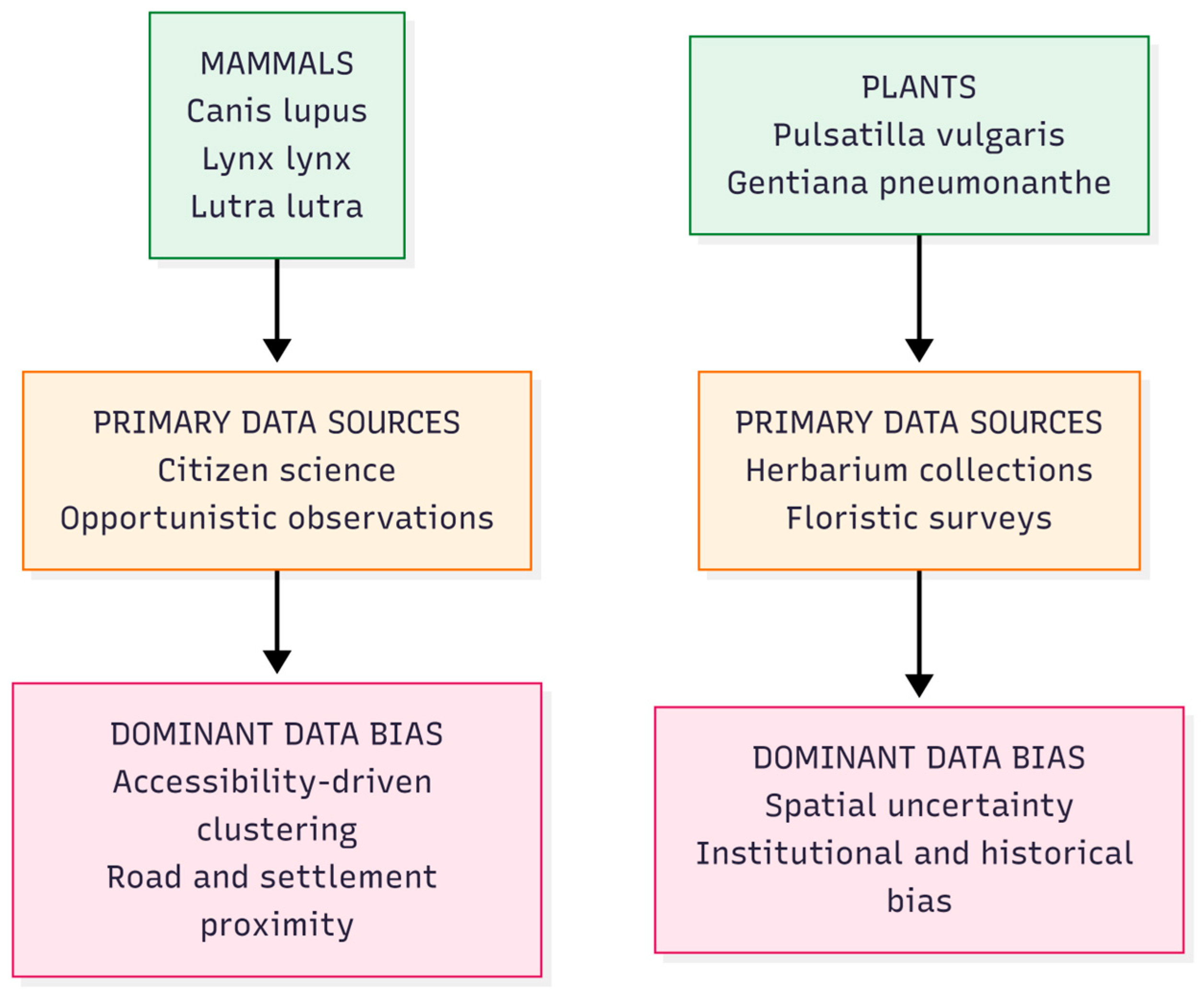
The relationships between the analyzed taxonomic groups, the primary sources of GBIF occurrence data, and the dominant types of bias motivating the methodological approach adopted in this study are summarized in Figure 1.

2. Materials

2.1. Study Area

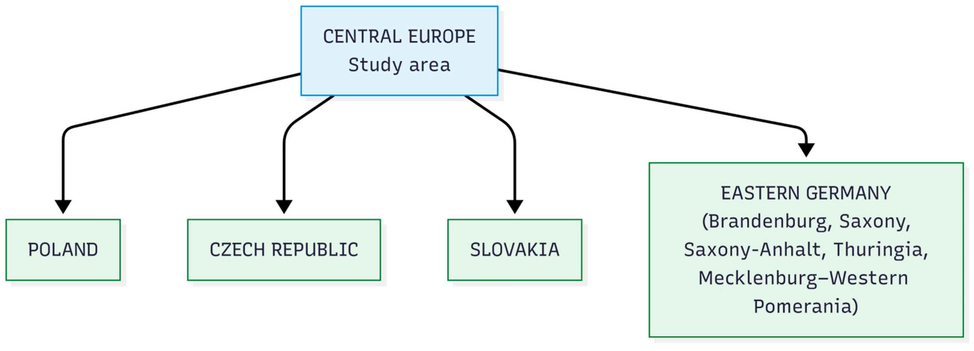
The study was conducted in Central Europe, encompassing four neighboring countries characterized by broadly similar climatic conditions, biogeographic history, and land-use patterns. The analyzed region includes the entire territories of Poland, the Czech Republic, and Slovakia, as well as the eastern part of Germany, specifically the federal states of Brandenburg, Saxony, Saxony-Anhalt, Thuringia, and Mecklenburg–Western Pomerania (Figure 2).

The study area spans a wide gradient of environmental and anthropogenic conditions, ranging from intensively managed agricultural landscapes and densely populated lowlands to extensive forest complexes, wetlands, and mountainous regions. This heterogeneity provides a suitable context for assessing spatial sampling bias and data quality issues in open-access biodiversity datasets, particularly those related to accessibility, observer effort, and historical data collection practices.

2.2. Target Species

The selected taxa intentionally represent contrasting dominant data sources in GBIF, with mammal records largely derived from opportunistic observations and monitoring programs, and plant records dominated by preserved herbarium specimens.

Five protected species representing two major taxonomic groups (mammals and vascular plants) were selected for analysis. Species selection was guided by their conservation relevance in Central Europe, the availability of occurrence records in GBIF, and their suitability for representing contrasting sources and structures of data bias.

The mammal group comprised Canis lupus (gray wolf), Lynx lynx (Eurasian lynx), and Lutra lutra (Eurasian otter). These species are of high conservation importance and are subject to extensive monitoring and reporting efforts across the study region. Their occurrence records originate from a combination of structured monitoring programs, professional surveys, and citizen science initiatives, making them well suited for assessing accessibility-driven spatial bias and observer-related clustering patterns.

The plant group included Pulsatilla vulgaris and Gentiana pneumonanthe. Both species are associated with habitat types of high conservation value, including semi-natural grasslands and wetlands, respectively. Their GBIF occurrence records are derived primarily from herbarium collections and floristic surveys, providing an opportunity to examine data quality and spatial bias patterns related to historical sampling practices, spatial precision, and the aggregation of records at identical or near-identical localities.

2.3. Occurrence Data

Species occurrence data were obtained from the Global Biodiversity Information Facility (GBIF). Records were downloaded using the GBIF data portal, and a Digital Object Identifier (DOI) was assigned to each download [25,26,27,28,29].

Only records meeting the following initial criteria were retained:

• presence of geographic coordinates;
• non-fossil basis of record;
• occurrence dates between 1950 and 2025.

No additional spatial or taxonomic filtering was applied at this stage in order to preserve a representative “raw” dataset suitable for subsequent data quality assessment and spatial bias analysis. The retained occurrence records originated from multiple data sources, including museum and herbarium collections, national and regional monitoring programs, and citizen science platforms, reflecting the heterogeneous nature of open-access biodiversity data.

3. Methods

3.1. Data Cleaning and Quality Control

I applied a systematic data-cleaning and quality-control procedure to identify and quantify common sources of error in GBIF occurrence records prior to spatial sampling bias assessment. The workflow was designed to be transparent and reproducible and was applied consistently to all five target species.

All records were standardized to a common coordinate reference system (WGS 84) to ensure spatial consistency across datasets [30,31].

Spatial validation of occurrence coordinates was performed. Records with potentially erroneous locations were identified and removed, including occurrences positioned at administrative or political centroids, institutional coordinates (e.g., museums and herbaria), zero coordinates, and duplicate coordinate pairs. Records sharing identical latitude and longitude values across multiple observations were treated as spatial duplicates and removed to reduce artificial spatial clustering. In addition, occurrence datasets were screened for extreme spatial outliers exhibiting unrealistic separation from the main cluster of records.

Taxonomic quality control was conducted by harmonizing species names against the GBIF taxonomic backbone. All records were checked for synonymy, outdated nomenclature, and taxonomic inconsistencies, with particular attention given to plant records derived from historical herbarium collections. Records that could not be confidently assigned to the accepted taxon were excluded from further analysis.

Both raw and cleaned versions of each dataset were retained. The number of records removed at each cleaning step was documented and subsequently summarized to allow direct comparison of data loss and dominant error types among species and taxonomic groups. The cleaned datasets resulting from this procedure formed the basis for subsequent spatial sampling bias analyses.

3.2. Assessment of Spatial Sampling Bias

Spatial sampling bias in the cleaned occurrence datasets was quantified using nearest neighbor-based metrics to assess deviations from complete spatial randomness (CSR) [32,33]. Analyses were performed separately for each species and subsequently compared across taxonomic groups to identify consistent and contrasting patterns of spatial clustering.

For each species, the observed mean nearest neighbor distance ${\bar{r}}_{\mathrm{obs}}$ was computed as the average distance between each occurrence and its closest neighbor in geographic space. Distances were measured in a projected, equal-area CRS (ETRS89/LAEA Europe) and are reported in meters [34]. Computing nearest neighbor distances in a planar projection ensures metric consistency required by point-pattern methods.

To enable comparison across species with different numbers of records and spatial extents, ${\bar{r}}_{\mathrm{obs}}$ was normalized by the expected mean nearest neighbor distance under CSR (Clark–Evans) [35,36,37]. The nearest neighbor ratio provides a simple and interpretable summary of spatial clustering that is well suited for cross-taxon comparisons and for evaluating changes in spatial structure following data-cleaning procedures.

Let $n$ denote the number of occurrences within the analysis window $W$ and $A$ its area (m²), with intensity $\lambda =n/A$ (m⁻²). The expected distance is:

$$\mathbb{E}[r_{\mathrm{N}\mathrm{N}}]={\displaystyle \frac{1}{2·\sqrt{\lambda }}}={\displaystyle \frac{0.5}{\sqrt{n/A}}}=0.5\sqrt{{\displaystyle \frac{A}{n}}}.$$

(1)

The nearest neighbor ratio $R$ (hereafter NNR) was then calculated as $\mathrm{N}\mathrm{N}\mathrm{R}={\bar{r}}_{\mathrm{obs}}/\mathbb{E}\left[r_{\mathrm{NN}}\right]$. Values $<1$ indicate clustering relative to CSR, values $\approx 1$ suggest approximate spatial randomness, and values $>1$ indicate regularity.

In this context, NNR is used as a comparative indicator of sampling structure rather than as a test of ecological randomness, and low NNR values are expected even in high-quality datasets due to genuine species aggregation.

The analysis window $W$ was defined as the convex hull of species’ occurrences intersected with the study-area boundary, to avoid inflating $A$ with empty regions (a known issue when using bounding boxes).

Spatial bias metrics were computed after data quality filtering to assess residual clustering patterns in cleaned datasets. Comparisons of NNR values among species and between mammal and plant datasets were used to characterize taxon-specific differences in spatial sampling structure associated with contrasting data sources and collection practices.

3.3. Software and Computational Environment

All data processing and spatial analyses were conducted using open-source software. Data cleaning, data quality assessment, and spatial sampling bias analyses were performed using Python (version 3.13) within the Spyder environment (Anaconda distribution) on a 64-bit Windows operating system.

No specialized hardware or high-performance computing infrastructure was required, and the complete analytical workflow can be reproduced on commonly available research computing environments.

Conceptual figures and workflow schematics were prepared using Mermaid, an open-source text-based diagramming tool, enabling the generation of flowcharts and conceptual diagrams directly from code-like descriptions [38].

4. Results

4.1. Data Quality and Record Filtering

A summary of data retention and dominant sources of data loss for the analyzed mammal species is provided in

Table 1. Summary of data quality assessment and record retention for the analyzed mammal species based on GBIF occurrence data.

Species	Raw Records	Records Retained	Retention (%)	Main Source of Data Loss
Canis lupus	5256	3034	57.7	Duplicate coordinates
Lynx lynx	602	496	82.4	Missing coordinates/date
Lutra lutra	3851	3276	85.1	Duplicate coordinates

.

A substantial reduction in the number of occurrence records was observed during the data-cleaning process. For Canis lupus, 3034 records remained from an initial set of 5256 GBIF records, corresponding to a reduction of approximately 42%. The largest data loss resulted from the removal of records with missing coordinates or event dates (16.6%) and from the elimination of duplicate geographic coordinates (25.7%), highlighting pronounced spatial clustering in the raw dataset. In contrast, centroid-like coordinates and institutional locations contributed negligibly to data reduction, indicating a predominance of point-based observational records.

Data quality patterns differed among the three mammal species. After quality control, 58% of Canis lupus records, 82% of Lynx lynx records, and 85% of Lutra lutra records were retained. For Canis lupus, data loss was dominated by duplicate geographic coordinates, reflecting strong spatial clustering of observations. In contrast, Lynx lynx records exhibited relatively low duplication and were primarily affected by missing coordinates or event dates. The highest overall data retention was observed for Lutra lutra, with minimal loss due to missing metadata and a moderate proportion of duplicate records, consistent with structured monitoring along river corridors.

To assess whether similar data quality patterns occur in plant occurrence datasets, an analogous analysis was conducted for two representative plant species. A summary of data retention and dominant sources of data loss for plant species is provided in

Table 2. Summary of data quality assessment and record retention for the analyzed plant species based on GBIF occurrence data.

Species	Raw Records	Records Retained	Retention (%)	Main Source of Data Loss
Pulsatilla vulgaris	14,883	6408	43.0%	Duplicate coordinates
Gentiana pneumonanthe	7186	3296	46.0%	Duplicate coordinates

.

Both plant species showed pronounced data loss during quality control, with 43% of Pulsatilla vulgaris and 46% of Gentiana pneumonanthe records retained after cleaning. In both cases, data reduction was overwhelmingly driven by the removal of duplicate geographic coordinates, reflecting the common practice of assigning identical coordinates to multiple herbarium specimens originating from the same locality. Missing coordinates, centroid-like locations, and institutional records played a negligible role in data loss, indicating high metadata completeness but limited spatial uniqueness of plant occurrence records.

The dominant filtering criteria differed systematically between taxa and reflect fundamental differences in data provenance. In mammals, record loss was driven by repeated observations of the same locations, consistent with monitoring and citizen science reporting. In contrast, for plant species, duplicate coordinates primarily reflect the aggregation of multiple preserved specimens originating from identical historical localities, rather than repeated ecological observations.

4.2. Spatial Bias in Occurrence Records

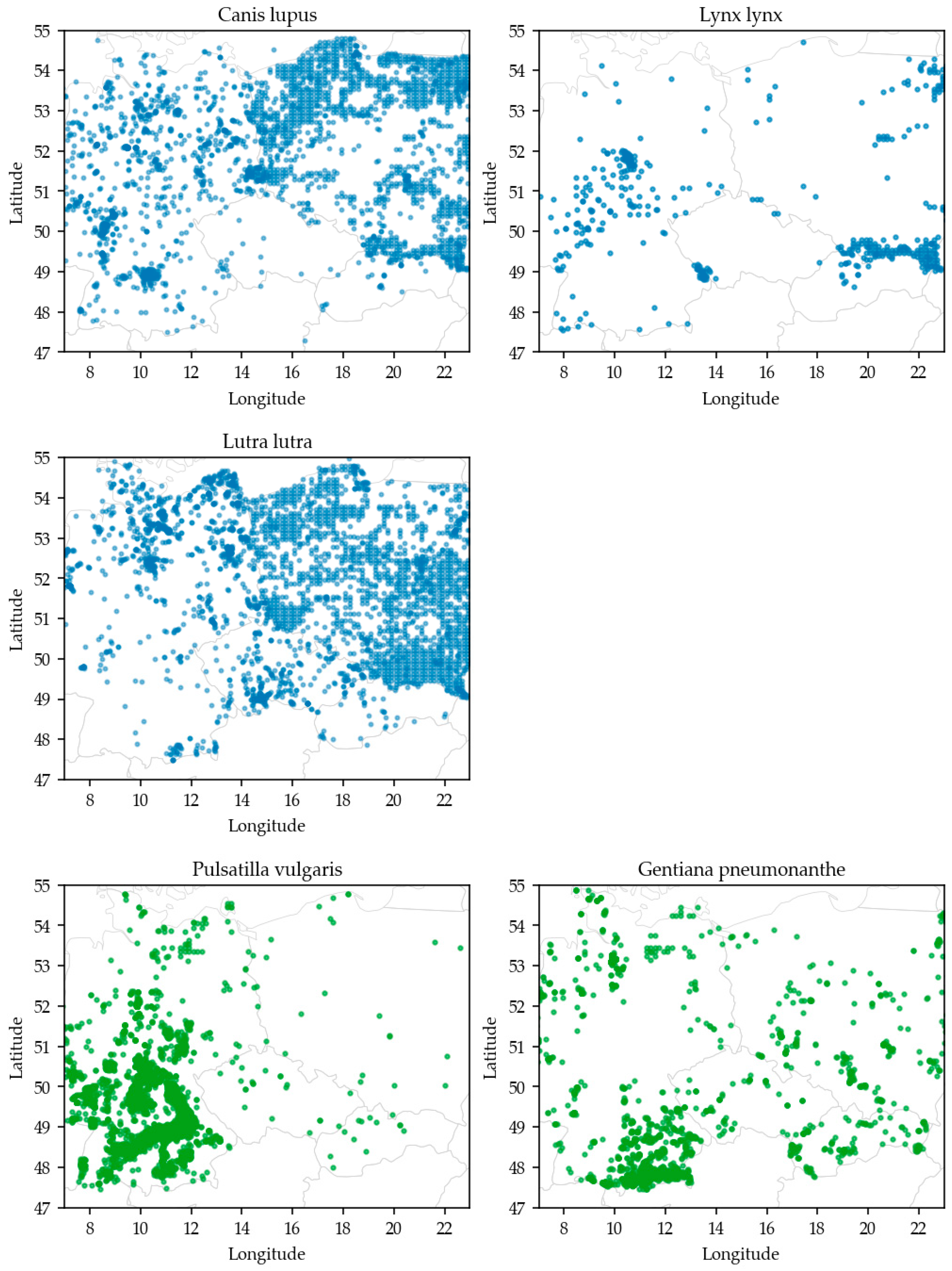
Following data quality control, the spatial distribution of retained occurrence records was examined to assess the presence and magnitude of spatial sampling bias. Despite the removal of duplicate coordinates and other low-quality records, occurrence points remained unevenly distributed across the study region for all analyzed species. This indicates that data quality filtering alone does not remove the uneven spatial structure associated with sampling effort, and that spatial clustering persists even in cleaned datasets.

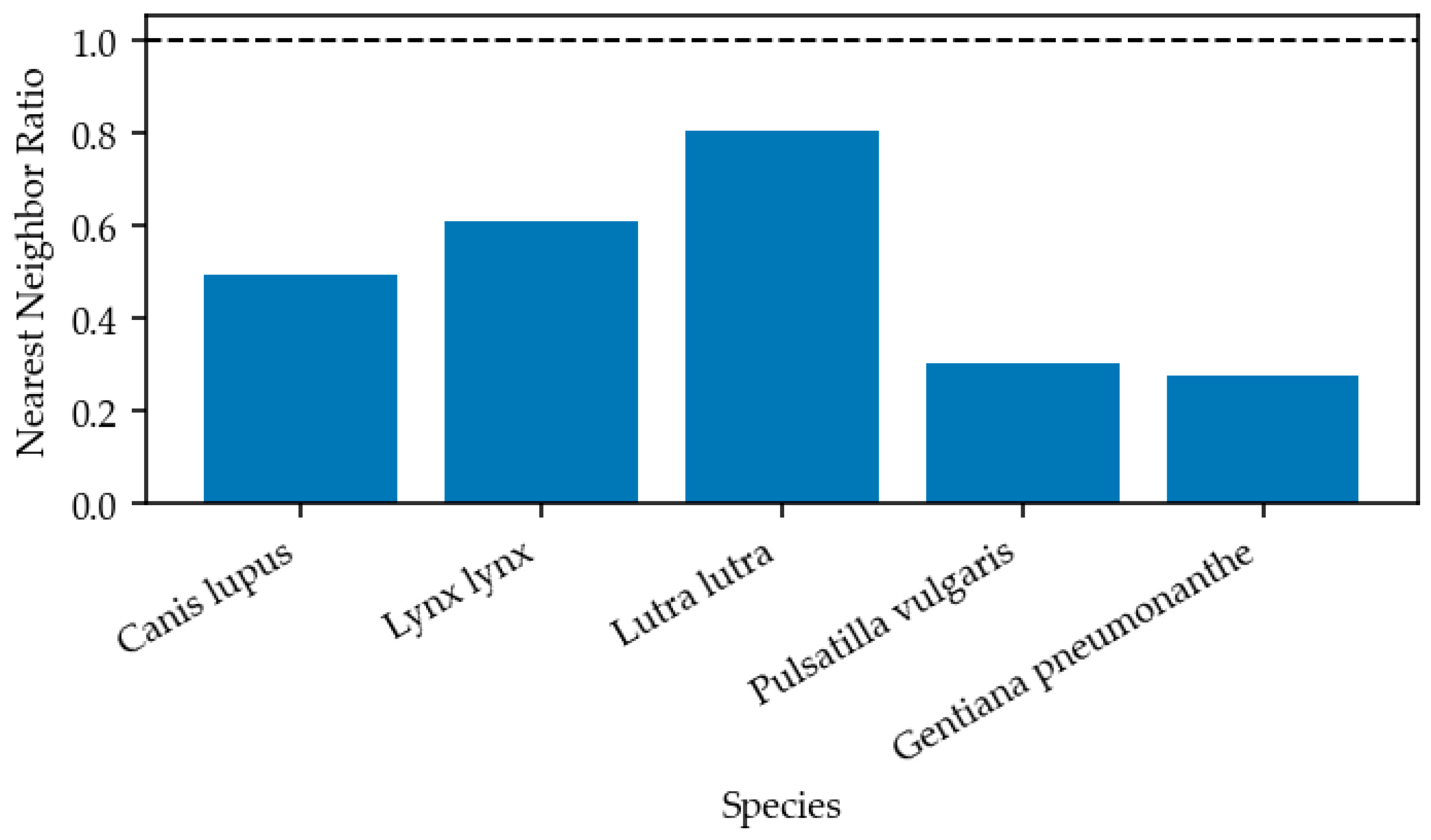
Nearest neighbor distance analysis revealed pronounced spatial clustering across all analyzed species, as indicated by nearest neighbor ratio (NNR) values substantially below unity (

Table 3. Nearest neighbor metrics for cleaned GBIF records.

Species	Mean NND (Observed, km)	Mean NND (Expected, km)	NNR (Naive)	NNR (Guard)
Canis lupus	8.2	16.58	0.49	0.41
Lynx lynx	11.95	19.64	0.61	0.58
Lutra lutra	7.12	8.88	0.80	0.80
Pulsatilla vulgaris	1.67	5.51	0.30	0.31
Gentiana pneumonanthe	2.25	8.16	0.28	0.27

). Spatial clustering patterns quantified using NNR are illustrated in Figure 3.

Among mammal species, the strongest spatial clustering was observed for Canis lupus (NNR = 0.49; guard-region NNR = 0.41), followed by Lynx lynx (0.61; 0.58) and Lutra lutra (0.80; 0.80). In contrast, plant species exhibited substantially lower NNR values, with Pulsatilla vulgaris (0.30; 0.31) and Gentiana pneumonanthe (0.28; 0.27), indicating highly clustered spatial distributions of retained occurrence records. The close correspondence between naive and guard-region NNR values for plant species, and the larger differences observed for mammals, reflect the stronger influence of window-boundary effects in wide-ranging mammalian datasets. These patterns remained evident despite prior data quality filtering and were consistent across the study region.

To evaluate the effect of data cleaning on spatial clustering, nearest neighbor ratios were also calculated for raw occurrence datasets prior to quality control (

Table 4. Comparison of nearest neighbor ratio (NNR) values calculated for raw and cleaned GBIF occurrence records.

Species	Records (Raw)	Records (Cleaned)	NNR (Raw)	NNR (Cleaned)
Canis lupus	5256	3034	0.33	0.49
Lynx lynx	602	496	0.53	0.61
Lutra lutra	3851	3276	0.73	0.80
Pulsatilla vulgaris	14,883	6408	0.06	0.30
Gentiana pneumonanthe	7186	3296	0.13	0.28

).

The spatial distribution of retained occurrence records for all species is illustrated in Figure 4.

Data cleaning consistently increased NNR values across all species, indicating the removal of extreme spatial artifacts associated with duplicate and erroneous coordinates. However, even after cleaning, NNR values remained well below unity, demonstrating that pronounced spatial sampling bias persists in GBIF occurrence data.

The strongest relative increase in NNR following data cleaning was observed for plant species, reflecting the high prevalence of duplicated geographic coordinates associated with herbarium-based records.

5. Discussion

5.1. Data Quality Patterns and Taxon-Specific Biases in GBIF Occurrence Data

The results reveal pronounced taxon-specific differences in the structure and dominant sources of bias in GBIF-derived occurrence datasets. Although identical quality-control procedures were applied across all analyzed species, both the magnitude and underlying causes of data loss differed substantially between mammal and plant taxa.

For large mammal species, data loss was primarily associated with spatial clustering and duplicate geographic coordinates, particularly in Canis lupus. This pattern likely reflects the combined influence of citizen science contributions, repeated monitoring of the same locations, and the high social and management relevance of large carnivores, which tend to attract repeated observations from identical or nearby locations. In contrast, Lynx lynx exhibited a markedly lower proportion of duplicate records and higher overall data retention, consistent with its lower population density, more cryptic behavior, and stronger reliance on structured monitoring programs. The intermediate pattern observed for Lutra lutra further supports this interpretation, as repeated observations along river corridors resulted in moderate spatial duplication without the extreme clustering observed for C. lupus.

In plant species, a fundamentally different data quality profile emerged. For both Pulsatilla vulgaris and Gentiana pneumonanthe, data loss was overwhelmingly driven by the removal of duplicate geographic coordinates, despite high metadata completeness and negligible contributions from centroid-like locations or institutional records. Unlike mammals, these duplicates do not reflect repeated ecological observations, but rather the assignment of identical coordinates to multiple herbarium specimens originating from the same locality. While this practice is taxonomically and historically justified, it substantially reduces the effective spatial resolution of plant occurrence datasets and may artificially inflate sampling intensity at specific locations if not explicitly addressed.

Importantly, the present results demonstrate that superficially similar filtering outcomes, such as the removal of duplicate coordinates, can arise from fundamentally different data-generating processes across taxonomic groups. Treating such filters as purely technical preprocessing steps risks obscuring biologically meaningful differences in sampling structure. Explicit reporting and interpretation of data quality patterns, as performed here, therefore provide essential context for subsequent spatial bias assessment and conservation-oriented spatial analyses.

Overall, these findings underscore that no single data-cleaning strategy can be universally optimal across taxa. Instead, quality control should be understood as an integral component of ecological inference, where the interpretation of filtered occurrence records is inseparable from the biology of the study organisms and the practices by which their data are collected.

Additionally, obtained results demonstrate that the impact of data cleaning cannot be interpreted independently of data source, as identical filtering criteria may remove fundamentally different types of information in observational versus specimen-based datasets.

5.2. Implications of Spatial Bias for Species Distribution Modelling and Conservation Analyses

It is important to emphasize that the persistence of spatial clustering after data cleaning does not indicate residual error but reflects the combined effects of biological aggregation and non-random sampling effort.

The spatial bias patterns identified in this study have important implications for downstream ecological analyses, particularly species distribution modeling (SDM) and conservation-oriented spatial assessments. The pronounced clustering detected across all analyzed species, even after rigorous data quality filtering, indicates that cleaned GBIF occurrence datasets cannot be assumed to approximate random or uniformly sampled representations of species’ geographic ranges.

Importantly, spatial randomness is neither expected nor desirable in ecological datasets, and the persistence of spatial clustering should not be interpreted as a failure of data cleaning, but as an inherent property of both species ecology and human sampling behavior.

An additional component of the observed spatial structure is the uneven density of occurrence records among countries within the study region. This pattern likely reflects a combination of genuine differences in species distribution and habitat availability, as well as country-level variation in sampling intensity, monitoring frameworks, institutional capacity, and data mobilization practices. Even within a relatively homogeneous biogeographic region such as Central Europe, national differences in biodiversity monitoring traditions and data-sharing policies can strongly influence the spatial density of available records. Disentangling ecological gradients from institutional and socio-cultural drivers of sampling effort would require independent effort metrics or structured monitoring data, which lies beyond the scope of the present study.

For mammal species, spatial clustering likely reflects a combination of uneven monitoring effort, repeated observations at accessible locations, and the influence of targeted survey programs. The strong clustering observed for Canis lupus suggests that SDMs calibrated directly on uncorrected occurrence data may overemphasize intensively sampled regions, potentially leading to biased estimates of habitat suitability and range extent. In contrast, the more dispersed patterns observed for Lynx lynx and Lutra lutra indicate comparatively lower sampling bias, although deviations from complete spatial randomness remain evident.

Plant species exhibited even stronger spatial clustering, as reflected by substantially lower nearest neighbor ratio values. Without appropriate bias-aware preprocessing, such clustering can artificially inflate the influence of a limited number of locations in SDMs and spatial prioritization analyses, particularly when presence-only modeling approaches are employed.

These results emphasize that data quality control and spatial bias correction should be treated as distinct and complementary steps in biodiversity data preprocessing. While standard filtering procedures effectively remove erroneous or low-quality records, they do not address the non-random spatial structure inherent in many occurrence datasets. Methods such as spatial thinning, bias-aware background sampling, or weighting schemes are therefore essential to mitigate the effects of clustering and to improve the robustness and ecological interpretability of SDM outputs.

Comparing naïve and guard-region nearest neighbor ratios provides additional insight into spatial structure. For mammal species, guard-region NNR values were consistently lower than their naïve counterparts (e.g., 0.49 → 0.41 for Canis lupus; 0.61 → 0.58 for Lynx lynx), indicating that part of the apparent spatial dispersion observed under the naïve metric was driven by edge effects in the convex hull window. This pattern reflects the wide geographic extent and irregular boundaries of mammal occurrence patterns, where points located near the perimeter of the study extent inflate the expected nearest neighbor distance. In contrast, plant species showed minimal differences between naïve and guard-region NNR values (e.g., Pulsatilla vulgaris: 0.30 → 0.31; Gentiana pneumonanthe: 0.28 → 0.27), demonstrating that their already highly clustered spatial structure is largely unaffected by window geometry. These findings underscore that the impact of edge effects is taxon-dependent and should be explicitly evaluated when assessing sampling bias. For taxa with broad, irregular ranges, such as large mammals, the use of guard-region or edge-corrected metrics provides a more conservative and robust estimate of spatial clustering, whereas for herbarium-derived plant datasets the difference is negligible owing to strong intrinsic clustering.

From a conservation perspective, failure to account for spatial bias may lead to misleading conclusions regarding species’ distribution patterns, habitat associations, and conservation priorities. Explicit quantification and transparent reporting of spatial bias, as demonstrated in this study, provide a robust methodological foundation for informed analytical choices and enhance the credibility and reproducibility of biodiversity analyses based on opportunistic occurrence data.

5.3. Implications for Monitoring Design

My findings highlight clear opportunities for improving biodiversity monitoring strategies. Identifying spatial biases and collector hotspots can directly support the optimization of future sampling schemes, especially in regions systematically underrepresented in herbarium and citizen science data. Targeted supplementary sampling in “cold spots” may substantially improve representativeness.

5.4. Implications for SDM Background Sampling

Bias-aware background generation, e.g., using effort surfaces or bias files can mitigate distortions introduced by uneven collector activity. My analysis demonstrates that quantifying spatial sampling structure can inform more realistic background sampling strategies, ultimately improving predictive performance and reducing overfitting to sampling artifacts.

5.5. Study Limitations

The two vascular plant species analyzed in this study were selected as representative examples of habitat-specialist taxa whose GBIF records are dominated by preserved herbarium specimens. However, vascular plants encompass a wide range of taxonomic complexity, ecological strategies, and recording traditions. Taxonomically complex genera, highly charismatic species, or extreme floristic rarities may exhibit distinct data quality profiles and spatial sampling structures due to frequent misidentification, taxonomic instability, or highly targeted collection effort. Consequently, the plant-specific patterns reported here should be interpreted as illustrative rather than universally representative of all vascular plant taxa.

Despite the robustness of the proposed workflow, several limitations must be acknowledged to contextualize the interpretation of our results.

First, herbarium-derived occurrence data are subject to georeferencing uncertainty, both due to historical imprecision and the retrospective assignment of coordinates to legacy specimens and bias-inferred clustering structure.

Second, the study does not incorporate explicit environmental drivers such as climatic gradients, land-use patterns, or habitat accessibility. Consequently, the observed sampling structures may conflate collector behavior with underlying ecological heterogeneity.

Third, no external comparison with systematic national monitoring schemes was conducted. Such programs offer structured sampling designs and could serve as an important benchmark to quantify the absolute magnitude of sampling bias in opportunistic collections.

Finally, the nearest neighbor ratio, while informative, cannot disentangle genuine ecological clustering from observer-induced aggregation, nor distinguish high-intensity collection hotspots from local environmental attractors. Future work should combine NNR with effort-corrected metrics.

6. Conclusions

My study emphasizes that understanding the spatial structure of opportunistic biodiversity data is essential for producing reliable ecological inference. The introduced framework provides tools that can support more transparent and bias-aware biodiversity management, guide better SDM background sampling, and inform data curation strategies for repositories such as GBIF. By making sampling heterogeneity explicit, future research can integrate collector behavior, environmental drivers, and structured monitoring to build more robust, interpretable models of biodiversity patterns.