Anomaly Detection Utilizing One-Class Classification—A Machine Learning Approach for the Analysis of Plant Fast Fluorescence Kinetics

Abstract

The analysis of fast fluorescence kinetics, specifically through the JIP test, is a valuable tool for identifying and characterizing plant stress. However, interpreting OJIP data requires a comprehensive understanding of their underlying theory. This study proposes a Machine Learning-based approach using a One-Class Support Vector Machine anomaly detection model to effectively categorize OJIP measurements into “normal”, representing healthy plants, and “anomalies”. This approach was validated using a previously published dataset. A subgroup of the identified “anomalies” was clearly linked to stress-induced reductions in photosynthesis. Furthermore, the percentage of these “anomalies” showed a meaningful correlation with both the progression and severity of stress. The results highlight the still largely unexploited potential of Machine Learning in OJIP analysis.

1. Introduction

When a dark-adapted leaf transitions to light, a rapid, polyphasic increase in chlorophyll fluorescence intensity is observed [1]. This progression swiftly moves from its initial value (O) through intermediate steps (J and I) to a peak (P) in less than a second. Step O represents the baseline fluorescence in the dark-adapted state, signifying the minimal fluorescence when all reaction centers are open. The subsequent O-J rise, occurring immediately upon exposure to light, corresponds to the quick reduction in Q_A and Q_B in Photosystem II (PSII). Following this, a more gradual J-I rise is observed, associated with the reduction in the plastoquinone pool. The fluorescence intensity reaches its zenith at P, indicating the peak reduction state of the electron transport chain involving both PSII and Photosystem I (PSI) [2]. Referred to as the OJIP curve, this rapid chlorophyll fluorescence rise kinetics provides a surprising wealth of information regarding PSII photochemical activity, electron transport events, and various photosynthetic processes. OJIP kinetics is also very sensitive to plant physiological conditions and effects of stress. Many stress factors, such as heat stress [3], cold stress [4], drought [5], salinity stress [6], heavy metal exposure [7], and nutrient deficiency [8], trigger distinct changes in OJIP curves. Thanks to its ease of measurement facilitated by user-friendly portable direct fluorescence fluorometers, OJIP analysis has gained widespread recognition as a powerful tool for studying plant photosynthesis and plant stress [9].

Proposed by Strasser in 1995 and perfected since then, the JIP test is a popular method for translating OJIP fluorescence signals into a large number of numerical biophysical parameters that can be used to compare between plant groups, as well as to classify and quantify the effects of stress. (For a thorough review of JIP test, see Tsimilli-Michael’s review in 2020 [10].) Nevertheless, interpreting these parameters can be difficult, particularly for those without a thorough understanding of the underlying theory. Many biophysical parameters derived from the JIP test rely on certain specific assumptions, and misunderstanding or neglecting these assumptions and their limitations can lead to erroneous or oversimplified interpretations [11]. For the benefit of non-expert users, efforts have been made to establish universal metrics that reliably reflect plant photosynthetic and physiological conditions. One of the most popular metrics is the Performance Index, PI_ABS, introduced as a product of terms expressing energy bifurcations, from the absorption events to the reduction of the intersystem electron transport chain [1]. Other variants of PI_ABS include the Structure–Function Index, SFI_ABS [12]; Total Performance Index, PI_TOTAL; and the Driving Forces, DF_ABS and DF_TOTAL [13]. There are also several OJIP-based indices tailored to specific types of stress, such as the Chill Factor Index, CFI [14]; Drought Factor Index, DFI [15]; Heat-Resistance Index, HRI [16]; and Heat Sensitivity Index, HIS [17]. Additionally, Duarte et al. [18] suggested a different methodology where distinct parameters obtained from the JIP test are combined mathematically into a single integrated biomarker response (IBR). It is worth noting that these metrics’ performance differs significantly among various stress types and plant species. While some stress metrics clearly correlate with the level of stress, in other cases, stress may or may not lead to detectable changes [19].

The utilization of Machine Learning (ML) techniques for analyzing OJIP curves presents a highly promising approach that is yet to be widely adopted. Due to its remarkable capacity to employ computer algorithms for extracting valuable insights from complex data, revealing hidden patterns, and offering precise predictions, the Machine Learning Revolution has gained substantial momentum in the last decade, profoundly reshaping various industries and sparking innovation across diverse applications [20]. In the realm of chlorophyll fluorescence measurements and OJIP analysis, ML has begun to make impactful strides. Principal Component Analysis (PCA) is employed to simplify OJIP data, facilitating visualization and the identification of data clusters [21]. Goltsev et al. [22] utilized Artificial Neural Networks (ANNs) to accurately predict relative water content based on chlorophyll fluorescence data. Combining PCA, Hierarchical k-means clustering, and Super-Organizing Maps (sSOMs), Kalaji et al. [23] accurately identified various levels of microelement deficiencies in rapeseed plants. Least-Squares Support Vector Machine (LS-SVM) enables the detection of citrus greening disease, a severe ailment affecting citrus [24]. These examples showcase the potential of ML in analysis of fast fluorescence kinetics data.

However, there are several complicating factors that could potentially challenge the accurate prediction capability of ML models. First, the high diversity of stress responses adds an additional layer of complexity to the picture. The plant stress response forms a highly intricate network that varies significantly depending on both biological and abiotic conditions. Many ML models for stress detection are multiclass classifiers trained on a predefined set of stressed plants [22,23,24]. If future stressed plants differ from the training batch (for example, due to genetic variations, differences in growth conditions, and presence of other stressors), the model may no longer function effectively. Another challenge arises from the spatial heterogeneity of stressed plants. In stressed plants, not all positions are equally affected, and some positions remain seemingly “healthy” [25,26,27]. Most OJIP measuring devices, including the widely used PocketPEA by Hansatech, are point-measurement devices which collect data from a single spot on the leaf. When measuring a stressed plant, while many measurements will correctly reflect the reduction in photosynthesis due to stress, a certain percentage of the measurements may still reflect normal conditions. Such heterogeneity makes it difficult to interpret the data. Last but not least, most published ML-based OJIP analysis models are based on parameters calculated from JIP tests, which are derived rather than directly measured. The validity of these parameters is contingent on numerous assumptions and constraints, which may or may not hold true under stress conditions.

To overcome challenges in analyzing fast fluorescence kinetics data, we recommend using a one-class classification approach utilizing OJIP curve’s raw data. One-class classification is an ML-based technique normally used for anomaly/outlier detection. This method entails training a model using only data from a single class (hence the name) to identify the standard pattern and its boundaries. The model then detects data points that deviate significantly from this standard pattern and identifies them as “outliers” [28]. Similarly, in our approach, we initially train a model using only OJIP curves from healthy plants to establish the standard OJIP pattern. Stress causes deviations from this pattern that are classified by the model as “anomalies”. This approach has several advantages. The relative consistency in OJIP patterns among healthy plants of the same species/cultivars strengthens the one-class classification model, making it more effective in discerning anomalies. In contrast to multiclass classification, where models are trained on data from specific types of stress, single-class anomaly detection allows for a more comprehensive detection of theoretically all types and severities of stress. Additionally, it accommodates the spatial heterogeneity of stressed plants, allowing for the accurate identification and separation of ostensibly “healthy” instances within measurements of stressed plants. Finally, the exclusive reliance on raw OJIP curve data frees the forecasting model from the constraints of the underlying assumptions associated with the JIP test’s theory and increases its objectivity. It is important to emphasize that the designation of a measurement as “anomaly” merely signifies its divergence from the conventional OJIP pattern and should not be automatically interpreted as indicative of stress. A multitude of processes in plants, including acclimatization to new conditions or intrinsic physiological processes such as flowering, are commonly associated with alterations in photosynthetic behaviors. Nevertheless, these processes are not typically regarded as stress.

In this study, we established a one-class classification model using OJIP data exclusively from healthy lettuce (Lactuca sativa Larissa) plants. This model was then employed to predict the photosynthetic status of lettuce plants throughout their cultivation, classifying them as either “normal” or “anomaly”. The prediction results and how they change throughout the year, in different growing conditions (both in the field and greenhouse), and when influenced by an external factor—namely, the presence of a radiofrequency electromagnetic field (RF-EMF)—would elucidate the feasibility of this novel approach.

2. Results and Discussion

2.1. Data Overview

A total of 1580 OJIP measurements from our previous study [29] were used in this study, including 864 from the greenhouse experiment and 716 from the field experiments. Each experiment began with the first measurement on 3-week-old plants fresh from the greenhouse that we assumed to be perfectly healthy. A total of 228 initial measurements were taken. Further measurements were taken over the next 4 weeks. The detailed distribution of measurements over time is shown in

Table 1. Overview of OJIP measurements used in this study.

	Field Experiments	Greenhouse Experiment	Total
Initial measurements	120	108	228
Week 1	80	108	188
Week 2	199	216	415
Week 3	159	216	375
Week 4	158	216	374
Total	716	864	1580

.

2.2. Screening of “Anomalies” for Model Fine-Tuning

Any classification model needs to be fine-tuned to balance Type I (false positive) and Type II (false negative) errors. In the case of a one-class classification model, the model is trained only on data from one class (healthy, i.e., “normal”, plants), so only Type I (“normal” misidentified as “anomalies”) error can be assessed. In order to assess Type II error (“anomalies” misidentified as “normal”), it is necessary to use data from the “anomaly” class as well. Several data points from our data can be identified as “anomalies” based on their F_V/F_M values. F_V/F_M represents the maximum quantum yield of photosystem II. Among the many parameters of chlorophyll fluorescence analysis, F_V/F_M is one of the most consistent values. It shows minimal variation in healthy plants regardless of differences in cultivar or growth conditions, which otherwise have a large influence on other parameters. It is well known that stress conditions can (but do not necessarily) reduce the values of F_V/F_M [2,30]. First, we analyzed the distribution of F_V/F_M values from the 228 initial measurements taken on 3-week-old plants, all of which were assumed to be perfectly healthy. All “normal” samples are expected to have F_V/F_M values within three standard deviations of this distribution. We then examined the F_V/F_M values from the remaining 1352 measurements. We found that 24 cases fell below this range (Figure 1). It is highly likely that these 24 cases represent a significant deviation from the typical pattern observed in healthy plants and therefore qualify as “anomalies”.

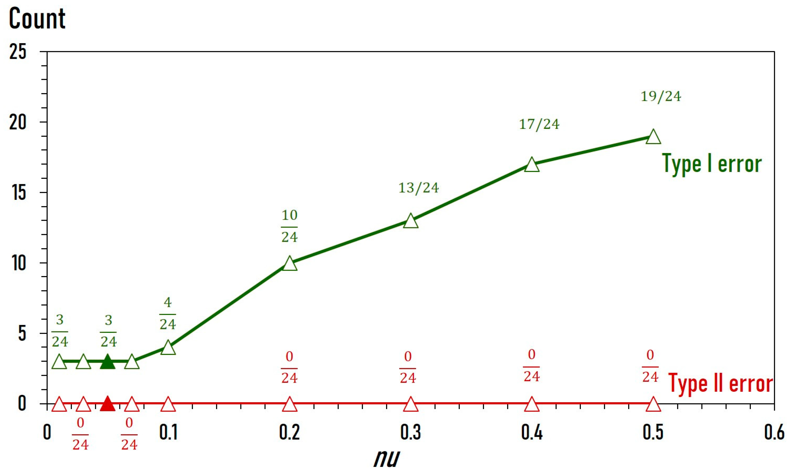
2.3. Training and Fine-Tuning of Classification Model

The 228 initial measurements described above were randomly divided into two subsets: 204 measurements for model training and 24 measurements for subsequent model fine-tuning. We trained our one-class classification model with the parameter nu varying between 0.01 and 0.5. nu represents a lower bound on the fraction of support vectors. Technically, a nu value of 0.1 means that at least 10% of the training samples are support vectors. It also represents the upper bound on the fraction of training errors. For example, a nu value of 0.1 means that the model can tolerate training errors of up to 10%. The optimal value of nu is determined by testing the model with a fine-tuning dataset (Figure 2). This dataset contains 48 data points, including the previously identified 24 ‘anomalies’ and an additional 24 “normal” data points. As a rule of thumb, increasing the nu value typically leads to less stringent screening for “anomalies” and a greater likelihood of “anomalies” being detected, while also increasing the risk of Type I error (“normal” misidentified as “anomalies”). Conversely, reducing the nu value reduces the risk of Type I errors but may result in some missed “anomaly” cases (i.e., increased risk of Type II errors).

The results of the model fine-tuning are shown in Figure 2. Out of all tested nu values, the models correctly identified all 24 “anomaly” cases as “anomalies”. On the other hand, all models misidentified some “normal” cases as “anomalies” to varying degrees. As expected, the number of misidentifications (Type I error) increases with the value of nu. Interestingly, lowering the value of nu below 0.1 did not improve performance. Consequently, the decision was made to adopt the nu value of 0.05 for all subsequent predictions.

2.4. Classification of the Remaining Data

In the following step, we applied the established model to classify all 1580 data points (

Table 2. Anomaly detection with all data. Number of “anomalies”/total number of measurements (percentage of “anomalies”).

	Field Experiments	Greenhouse Experiment	Total
Initial measurements	8/120 (6.7%)	6/108 (5.6%)	14/228
Week 1	26/80 (32.5%)	41/108 (38.0%)	67/188
Week 2	91/199 (45.7%)	50/216 (23.1%)	141/415
Week 3	121/159 (76.1%)	83/216 (38.4%)	204/375
Week 4	115/158 (72.8%)	123/216 (56.9%)	238/374
Total	361/716	303/864	664/1580

). Out of these, 664 measurements were marked as “anomalies”. The remaining 916 measurements were categorized as “normal”. Out of 228 initial measurements, 14 (6%) “anomalies” were detected.

2.5. Comparison Between “Normal” and “Anomaly” Measurements

Labeling a measurement as an “anomaly” only signifies that its OJIP curve deviates from the typical pattern observed in “normal” (i.e., healthy) measurements. To assess and compare the photosynthetic efficiency between the “anomaly” and “normal” groups, we conducted a standard JIP test to compare “normal” and “anomalies” in each experiment. A total of 20 different parameters were calculated from each OJIP curve: tFm, Area, F_O, F_M, F_V, F_O/F_M, F_V/F_M, F_V/F_O, V_j, V_i, dVG/dt_O, dV/dt_O, Sm, N, Sm/tFm, ABS/RC, TR_O/RC, ET_O/RC, RE_O/RC, and PI_ABS. For a more detailed understanding of the OJIP parameters presented, see Stirbet and Go-vindjee, 2011 [11]. In each experiment, the values were normalized by setting the mean of the “normal” samples to 1. We then plotted all normalized values on spider plots to visualize the difference between “abnormal” and “normal” groups (Figure 3).

Examining Figure 3, a noticeable pattern emerges: “anomalies” across all three field experiments consistently demonstrate a lower photosynthetic performance compared to “normal” measurements. This is evident in statistically significantly reduced values for F_V/F_M and PI_ABS (Figure 4). The distinction between these groups is maintained across various parameters, with “anomalies” consistently displaying lower values for Area, F_O, F_M, and F_V, and higher values for dV/dt_O, ABS/RC, and TRo/RC. Conversely, the comparison between “anomalies” and “normal” in the greenhouse experiment presents a very different picture. In this case, the “anomalies” exhibit statistically significantly higher PI_ABS and F_V/F_M (Figure 4). Additionally, “anomalies” in the greenhouse show lower values for dV/dt_O, N, and S_m/tF_M.

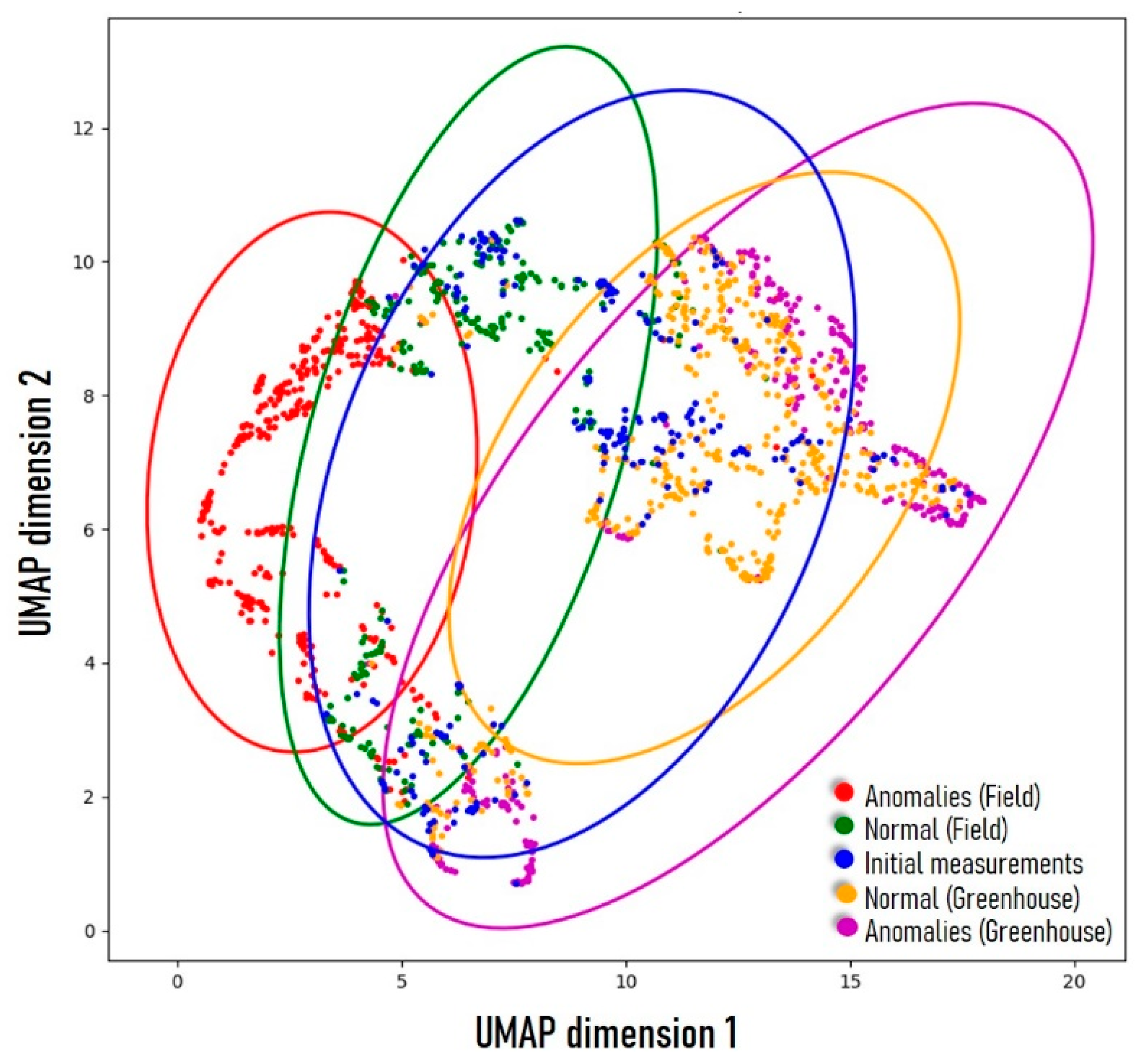
2.6. UMAP Visualization of All Measurements

To assess the interrelation among all measurements, we employed Uniform Manifold Approximation and Projection (UMAP) to project the entire dataset into a two-dimensional space, as illustrated in Figure 5. The observed pattern aligns consistently with other findings in this study. The initial measurements (blue dots), along with all “normal” measurements (green and orange dots), cluster at the center of the scatter plot, while the “anomalies” (red and magenta dots) are scattered towards the periphery. Notably, a distinct separation is evident between “anomalies” originating from the field experiments (red) and those from the greenhouse experiment (magenta), implying they are of fundamentally different natures.

2.7. k-Means Clustering of “Anomalies”

The UMAP analysis suggests that unsupervised clustering algorithms can differentiate between different types of “anomalies” in field and greenhouse experiments. Using the conventional k-means clustering, the detected “anomalies” were divided into two clusters: Cluster 1 includes 8 greenhouse “anomalies” (2.3%) and 345 field “anomalies” (97.7%), while Cluster 2 includes 295 greenhouse “anomalies” (94.9%) and 16 field “anomalies” (5.1%). These “anomalies” will be referred to as type 1 and 2 (

Table 3. Type 1 and 2 “anomalies”. Number of “anomalies” type 1/2/total number of measurements (percentage of “anomalies” type 1/2).

	Field Experiments		Greenhouse Experiment
	“Anomalies” Type 1	“Anomalies” Type 2	“Anomalies” Type 1	“Anomalies” Type 2
Initial measurements	8/120 (6.7%)	0/108 (0%)	0/120 (6.7%)	6/108 (0%)
Week 1	23/80 (28.8%)	3/80 (3.8%)	6/108 (5.6%)	35/108 (32.4%)
Week 2	80/199 (40.2%)	11/199 (5.5%)	0/216 (0%)	50/216 (23.1%)
Week 3	121/159 (76.1%)	0/159 (0%)	1/216 (0.5%)	82/216 (37.9%)
Week 4	113/158 (71.5%)	2/158 (1.3%)	1/216 (0.5%)	122/216 (56.5%)
Total	345/716	16/716	8/864	295/864

).

2.8. Comparison Between “Anomalies” Types 1 and 2

A comparison was made between “anomaly” types 1 and 2 using the standard JIP test to assess photosynthetic efficiency. The results are presented in Figure 6.

The analysis confirms that “anomalies” types 1 and 2 are fundamentally different in nature. Type 1 exhibit significantly lower photosynthetic performance compared to “normal” measurements. This is evident from lower values for Area, F_O, F_M, F_V, F_V/_FM, and PI_ABS, and higher values for dV/dt_O, ABS/RC, and TR_O/RC. On the other hand, type 2 “anomalies” exhibit better photosynthesis than the “normal” type, as evidenced by their statistically significantly higher PI_ABS. The presence of “anomaly” types in individual experiments is also noteworthy (Figure 7). Type 1 “anomalies” were prevalent in field experiments, while type 2 “anomalies” were only sporadic. The highest percentage of type 1 occurred in the field experiments conducted in September 2021 and August 2022, while the lowest percentage occurred in the June 2022 experiment. Furthermore, the percentage of type 1 “anomalies” in plants exposed to RF-EMF is consistently higher than in the control group. In the greenhouse experiment, type 2 was dominant. It is worth noting that the percentage of the dominant “anomaly” type tends to increase with cultivation time, typically peaking at the end of the experiment.

2.9. Interpretation of the Results

By combining the shifts in the “anomaly” types’ percentage during cultivation (Figure 7) with their comparison with each other and with “normal” measurements (Figure 6), a reasonable interpretation can be made.

Field experiments: Type 1 “anomalies” are caused by stress. The increased occurrence of type 1 “anomalies” appears to represent a progressive response to stress under field conditions. While plants were initially healthy at the start of the experiments, their photosynthetic efficiency gradually declined due to various environmental stress factors, giving rise to a discernible increase in the prevalence of type 1 “anomalies”. Notably, plants seemed to experience higher stress levels in September 2021 and August 2022 compared to June 2022, and this result can possibly be attributed to the low temperature in September 2021 and the heatwave at the beginning of August 2022 (for field experiment’s meteorological data, see [29]). Moreover, across three field experiments, the proportion of type 1 “anomalies” in plants exposed to RF-EMF is consistently greater than that in control plants. This observation aligns with previously published findings suggesting that RF-EMF exposure has detrimental effects on plant photosynthesis in field conditions [29].

Greenhouse experiment: Type 1 stress-related “anomalies” were remarkably absent in the greenhouse experiment, consistent with the expectation that plant cultivation in such controlled environments is generally stress-free. The emergence of type 2 anomalies under greenhouse conditions suggests an alternative cause. The observed increase in anomalies throughout cultivation time hints at a possible connection between type 2 anomalies and the plants’ acclimation from the greenhouse to the phytochamber conditions. Further research is needed to unravel the nature of these anomalies.

2.10. Summary and Outlook

The study aimed to test the feasibility of utilizing One-Class Support Vector Machine Classification for the analysis of plant fast fluorescence kinetics. After analyzing 1580 OJIP measurements, the model detected 664 “anomalies”, which can be further divided into 353 type 1 and 311 type 2 “anomalies”. There is strong evidence that type 1 “anomalies” may be caused by stress. The prevalence of type 1 “anomalies” correlates well with both the progression and severity of stress. Type 2 is not related to stress and is typically found only in greenhouse environments.

The detection and characterization of “anomalies” should not be seen as an alternative approach to the well-established JIP test. Rather, it provides complementary insight into the relative shape of the OJIP curves, providing additional information that is not captured by the parameters based on the JIP test. This approach bears some similarity to the conventional analysis of the semi-quantitative bands in the OJIP curve (K-, L-, and J-band [10]), but with a greater degree of flexibility that may allow for improved detection capabilities.

“Anomalies” should not automatically be interpreted as stress symptoms. While the results provide strong evidence that type 1 “anomalies” observed in all three field experiments are due to plant stress induced by environmental factors, type 2 “anomalies” observed in the stress-free greenhouse experiment do not show stress-related characteristics. The UMAP and k-means clustering results suggest that it is possible to use clustering algorithms to divide “anomalies” into distinct groups, providing an opportunity for a more in-depth analysis of their nature.

The proposed approach holds significant potential for practical applications, especially in plant stress research. The percentage of stress-related “anomalies” might serve as a useful indicator for the severity and progression of stress. Different stress types might manifest distinct types of “anomalies”, aiding in pinpointing the specific cause of stress. Furthermore, the power of this approach would be greatly enhanced in combination with the image-based OJIP technique, which has started gaining momentum in recent years [31,32,33]. This combination would provide insight into the percentage of “anomalies”, their groupings, and photosynthetic properties, as well as how these “anomalies” spread through the plant as stress progresses. This would provide a more comprehensive picture of the effects of stress on plants.

In summary, our analysis underscores the importance of integrating ML-based methodology with conventional OJIP analysis. This synergistic approach not only reveals hidden patterns but also provides valuable insights into the intricate ways in which plants respond to changes in their environments.

3. Materials and Methods

In this study, we used data from our previous research [29], in which the effects of RF-EMF exposure on lettuce plants under both indoor and outdoor conditions were investigated. All data are available in the Supplementary Materials.

3.1. Plant Cultivation

Lactuca sativa plants (cultivars Larissa, purchased from Kiepelkern, Bruno Nebelung GmbH, Everswinkel, Germany) were cultivated in soil pots in a greenhouse, maintaining temperatures between 19 °C and 23 °C and humidity at 50–60%, until they reached 3 weeks of age. Subsequently, they were either relocated to a phytochamber with controlled conditions (20 °C, 50% humidity, 16/8 h light/dark cycle) or an outdoor experimental field (coordinates 49°49′57.4″ N 8°34′22.2″ E), where cultivation continued until senescence. The greenhouse experiment was conducted in September 2022, while field cultivation took place in three batches: August–September 2021, June–July 2022, and August 2022. In each experiment, the plants were divided into two groups (9–10 plants each): one group exposed to RF-EMF (1880–1900 MHz DECT, and 2.4 and 5 GHz WLAN; power flux densities about 10,000 μW/m²), while the other served as the control group. Under greenhouse conditions, plants are anticipated to encounter minimal stress, whereas in field environments, they are subjected to a range of environmental stressors [29].

3.2. Measurements of Fast Chlorophyll Fluorescence Kinetics

The Pocket PEA device from Hansatech was used to measure the fast chlorophyll fluorescence kinetics of leaves (measurement time, one second; saturating light intensity, 3500 µmol/m².s). For outdoor conditions, measurements were conducted at a minimum of 3 h after sunset. In the greenhouse, measurements were taken at the conclusion of the dark phase. OJIP parameters were computed using the PEA Plus Version 1.13 software from Hansatech. Initial measurements commenced 48 h after the young plants were transferred to the experiment’s locations. Subsequently, plant measurements were taken at regular intervals (approximately two to three times a week) until senescence [29].

3.3. Data Overview and Data Pre-Processing

A total of 1580 OJIP measurements were utilized in this study, comprising 864 from the greenhouse experiment and 716 from field experiments. The investigation focused solely on the raw data of the OJIP curve, excluding all derived parameters. Nine features were extracted from each curve: baseline fluorescence intensity (F_O); peak fluorescence intensity (F_M); fluorescence intensities at five specific time marks (50 µs, 100 µs, 300 µs, 2 ms, and 30 ms—F1, F2, F3, F4, and F5); the time at which the maximum fluorescence value, F_M, was reached (Tfm); and the area above the fluorescence curve between F_O and F_M (Area) (Figure 8). All data underwent normalization using robust standardization.

$$X_{robuststandardized}={\displaystyle \frac{X-{Median}_{TRAIN}}{{IQR}_{TRAIN}}}$$

Median_TRAIN and IQR_TRAIN represent the median and interquartile range of the training dataset. The use of robust standardization ensures the effective capture of the central tendency and spread of the data while remaining resilient to the impact of outliers.

3.4. One-Class Support Vector Machine

Anomaly detection was executed utilizing the One-Class Support Vector Machine algorithm, with the Python code imported from Scikit-learn (sklearn.svm.OneClassSVM [34]). The code utilized default parameters, including kernel = “rbf”, degree = 3, gamma = “scale”, coef0 = 0.0, tol = 0.001, shrinking = True, cache_size = 200, verbose = False, and max_iter = −1. The parameter nu, representing an upper bound on the fraction of training errors and a lower bound of the fraction of support vectors, was fine-tuned using the fine-tuning dataset.

3.5. UMAP Data Visualization

In order to visualize the OJIP measurements in a lower-dimensional space and to enhance interpretability, Uniform Manifold Approximation and Projection (UMAP) was employed [35]. As a dimensionality reduction technique, UMAP shares similarities with PCA, yet it surpasses PCA by preserving not only the global structure but also the intricate local relationships within the data. This enhanced capability makes UMAP particularly adept at capturing complex, non-linear relationships present in the dataset. The UMAP algorithm is implemented through the umap-learn Python library [36]. Random seed state was set at random_state = 42 to ensure UMAP reproducibility.

3.6. k-Means Clustering

K-means clustering [37] was used to partition the detected “anomalies” into distinct subsets. The code used was imported from Scikit-learn (sklearn.cluster.KMeans; [34]). The code used default parameters, including init = “k-means + +”, n_init = “warn”, max_iter = 300, tol = 0.0001, verbose = 0, random_state = None, copy_x = True, and algorithm = “lloyd”. The optimal number of clusters was determined using the silhouette score (sklearn.metrics.silhouette_score), with the default settings: metric = “euclidean”, sample_size = None, and random_state = None.

3.7. Statistical Analysis

Student’s t-test and One-Way Analysis of Variance (ANOVA) with post hoc Tukey Honestly Significant Difference (HSD) test were applied to compare groups throughout the study. Statistical significance was assumed when p < 0.05. Statistical tests were performed with Jamovi and Microsoft Excel with Real Statistics Add-Ins.

References

1. Strasser, R.J.; Srivastava, A.; Govindjee. Polyphasic Chlorophyll a Fluorescence Transient in Plants and Cyanobacteria*. Photochem. Amp. Photobiol. 1995, 61, 32–42. [Google Scholar] [CrossRef]
2. Kalaji, H.M.; Schansker, G.; Ladle, R.J.; Goltsev, V.; Bosa, K.; Allakhverdiev, S.I.; Brestic, M.; Bussotti, F.; Calatayud, A.; Dąbrowski, P.; et al. Frequently asked questions about In Vivo chlorophyll fluorescence: Practical issues. Photosynth. Res. 2014, 122, 121–158. [Google Scholar] [CrossRef] [PubMed]
3. Mathur, S.; Jajoo, A.; Mehta, P.; Bharti, S. Analysis of elevated temperature—Induced inhibition of photosystem II using chlorophyll a fluorescence induction kinetics in wheat leaves (Triticum aestivum). Plant Biol. 2010, 13, 1–6. [Google Scholar] [CrossRef]
4. Yang, J.; Kong, Q.; Xiang, C. Effects of low night temperature on pigments, chl a fluorescence and energy allocation in two bitter gourd (Momordica charantia L.) genotypes. Acta Physiol. Plant. 2008, 31, 285–293. [Google Scholar] [CrossRef]
5. Jedmowski, C.; Brüggemann, W. Imaging of fast chlorophyll fluorescence induction curve (OJIP) parameters, applied in a screening study with wild barley (Hordeum spontaneum) genotypes under heat stress. J. Photochem. Photobiol. B Biol. 2015, 151, 153–160. [Google Scholar] [CrossRef]
6. Singh-Tomar, R.; Mathur, S.; Allakhverdiev, S.I.; Jajoo, A. Changes in PS II heterogeneity in response to osmotic and ionic stress in wheat leaves (Triticum aestivum). J. Bioenerg. Biomembr. 2012, 44, 411–419. [Google Scholar] [CrossRef]
7. Kalaji, H.M.; Loboda, T. Photosystem II of barley seedlings under cadmium and lead stress. Plant Soil Environ. 2007, 53, 511–516. [Google Scholar] [CrossRef]
8. Redillas, M.C.F.R.; Jeong, J.S.; Strasser, R.J.; Kim, Y.S.; Kim, J.-K. JIP analysis on rice (Oryza sativa cv Nipponbare) grown under limited nitrogen conditions. J. Korean Soc. Appl. Biol. Chem. 2011, 54, 827–832. [Google Scholar] [CrossRef]
9. Kalaji, H.M.; Jajoo, A.; Oukarroum, A.; Brestic, M.; Zivcak, M.; Samborska, I.A.; Cetner, M.D.; Łukasik, I.; Goltsev, V.; Ladle, R.J. Chlorophyll a fluorescence as a tool to monitor physiological status of plants under abiotic stress conditions. In Acta Physiologiae Plantarum; Springer Science and Business Media LLC: Berlin/Heidelberg, Germany, 2016; Volume 38. [Google Scholar] [CrossRef]
10. Tsimilli-Michael, M. Special issue in honour of Prof. Reto J. Strasser—Revisiting JIP-test: An educative review on concepts, assumptions, approximations, definitions and terminology. Photosynt. 2020, 58, 275–292. [Google Scholar] [CrossRef]
11. Stirbet, A. Govindjee On the relation between the Kautsky effect (chlorophyll a fluorescence induction) and Photosystem II: Basics and applications of the OJIP fluorescence transient. J. Photochem. Photobiol. B Biol. 2011, 104, 236–257. [Google Scholar] [CrossRef]
12. Srivastava, A.; Strasser, R.J.; Govindjee. Greening of Peas: Parallel Measurements of 77 K Emission Spectra, OJIP Chlorophyll a Fluorescence Transient, Period Four Oscillation of the Initial Fluorescence Level, Delayed Light Emission, and P700. Photosynthetica 1999, 36, 365. [Google Scholar] [CrossRef]
13. Tsimilli-Michael, M.; Strasser, R.J. In Vivo Assessment of Stress Impact on Plant’s Vitality: Applications in Detecting and Evaluating the Beneficial Role of Mycorrhization on Host Plants. Mycorrhiza 2008, 679–703. [Google Scholar] [CrossRef]
14. Strauss, A.J.; Krüger, G.H.J.; Strasser, R.J.; Heerden, P.D.R.V. Ranking of dark chilling tolerance in soybean genotypes probed by the chlorophyll a fluorescence transient O-J-I-P. Environ. Exp. Bot. 2006, 56, 147–157. [Google Scholar] [CrossRef]
15. Oukarroum, A.; Madidi, S.E.; Schansker, G.; Strasser, R.J. Probing the responses of barley cultivars (Hordeum vulgare L.) by chlorophyll a fluorescence OLKJIP under drought stress and re-watering. Environ. Exp. Bot. 2007, 60, 438–446. [Google Scholar] [CrossRef]
16. Jedmowski, C.; Bayramov, S.; Brüggemann, W. Comparative analysis of drought stress effects on photosynthesis of Eurasian and North African genotypes of wild barley. Photosynthetica 2014, 52, 564–573. [Google Scholar] [CrossRef]
17. Chen, S.; Yang, J.; Zhang, M.; Strasser, R.J.; Qiang, S. Classification and characteristics of heat tolerance in Ageratina adenophora populations using fast chlorophyll a fluorescence rise O-J-I-P. Environ. Exp. Bot. 2016, 122, 126–140. [Google Scholar] [CrossRef]
18. Duarte, B.; Pedro, S.; Marques, J.C.; Adão, H.; Caçador, I. Zostera noltii development probing using chlorophyll a transient analysis (JIP-test) under field conditions: Integrating physiological insights into a photochemical stress index. Ecol. Indic. 2017, 76, 219–229. [Google Scholar] [CrossRef]
19. Stirbet, A.; Lazár, D.; Kromdijk, J.; Govindjee, G. Chlorophyll a fluorescence induction: Can just a one-second measurement be used to quantify abiotic stress responses? Photosynthetica 2018, 56, 86–104. [Google Scholar] [CrossRef]
20. LeCun, Y.; Bengio, Y.; Hinton, G. Deep learning. In Nature; Springer Science and Business Media LLC: Berlin/Heidelberg, Germany, 2015; Volume 521, pp. 436–444. [Google Scholar] [CrossRef]
21. Kalaji, H.M.; Oukarroum, A.; Alexandrov, V.; Kouzmanova, M.; Brestic, M.; Zivcak, M.; Samborska, I.A.; Cetner, M.D.; Allakhverdiev, S.I.; Goltsev, V. Identification of nutrient deficiency in maize and tomato plants by In Vivo chlorophyll a fluorescence measurements. Plant Physiol. Biochem. 2014, 81, 16–25. [Google Scholar] [CrossRef]
22. Goltsev, V.; Zaharieva, I.; Chernev, P.; Kouzmanova, M.; Kalaji, H.M.; Yordanov, I.; Krasteva, V.; Alexandrov, V.; Stefanov, D.; Allakhverdiev, S.I. Drought-induced modifications of photosynthetic electron transport in intact leaves: Analysis and use of neural networks as a tool for a rapid non-invasive estimation. Biochim. Biophys. Acta Bioenerg. 2012, 1817, 1490–1498. [Google Scholar] [CrossRef]
23. Kalaji, H.M.; Bąba, W.; Gediga, K.; Goltsev, V.; Samborska, I.A.; Cetner, M.D.; Dimitrova, S.; Piszcz, U.; Bielecki, K.; Karmowska, K. Chlorophyll fluorescence as a tool for nutrient status identification in rapeseed plants. Photosynth. Res. 2017, 136, 329–343. [Google Scholar] [CrossRef] [PubMed]
24. Weng, H.; Liu, Y.; Captoline, I.; Li, X.; Ye, D.; Wu, R. Citrus Huanglongbing detection based on polyphasic chlorophyll a fluorescence coupled with machine learning and model transfer in two citrus cultivars. Comput. Electron. Agric. 2021, 187, 106289. [Google Scholar] [CrossRef]
25. Bresson, J.; Vasseur, F.; Dauzat, M.; Koch, G.; Granier, C.; Vile, D. Quantifying spatial heterogeneity of chlorophyll fluorescence during plant growth and in response to water stress. Plant Methods 2015, 11, 23. [Google Scholar] [CrossRef] [PubMed]
26. Huang, X.; Chen, H.; Chen, H.; Fan, C.; Tai, Y.; Chen, X.; Zhang, W.; He, T.; Gao, Z. Spatiotemporal Heterogeneity of Chlorophyll Content and Fluorescence Response within Rice (Oryza sativa L.) Canopies under Different Cadmium Stress. Agronomy 2022, 13, 121. [Google Scholar] [CrossRef]
27. Arief, M.A.A.; Kim, H.; Kurniawan, H.; Nugroho, A.P.; Kim, T.; Cho, B.-K. Chlorophyll Fluorescence Imaging for Early Detection of Drought and Heat Stress in Strawberry Plants. Plants 2023, 12, 1387. [Google Scholar] [CrossRef]
28. Seliya, N.; Abdollah Zadeh, A.; Khoshgoftaar, T.M. A literature review on one-class classification and its potential applications in big data. J. Big Data 2021, 8, 122. [Google Scholar] [CrossRef]
29. Tran, N.T.; Jokic, L.; Keller, J.; Geier, J.U.; Kaldenhoff, R. Impacts of Radio-Frequency Electromagnetic Field (RF-EMF) on Lettuce (Lactuca sativa)—Evidence for RF-EMF Interference with Plant Stress Responses. Plants 2023, 12, 1082. [Google Scholar] [CrossRef]
30. Shomali, A.; Aliniaeifard, S.; Bakhtiarizadeh, M.R.; Lotfi, M.; Mohammadian, M.; Vafaei Sadi, M.S.; Rastogi, A. Artificial neural network (ANN)-based algorithms for high light stress phenotyping of tomato genotypes using chlorophyll fluorescence features. Plant Physiol. Biochem. 2023, 201, 107893. [Google Scholar] [CrossRef]
31. Jedmowski, C.; Ashoub, A.; Brüggemann, W. Reactions of Egyptian landraces of Hordeum vulgare and Sorghum bicolor to drought stress, evaluated by the OJIP fluorescence transient analysis. Acta Physiol. Plant. 2012, 35, 345–354. [Google Scholar] [CrossRef]
32. Küpper, H.; Benedikty, Z.; Morina, F.; Andresen, E.; Mishra, A.; Trtílek, M. Analysis of OJIP Chlorophyll Fluorescence Kinetics and QA Reoxidation Kinetics by Direct Fast Imaging. Plant Physiol. 2018, 179, 369–381. [Google Scholar] [CrossRef]
33. Morales, L.O.; Shapiguzov, A.; Safronov, O.; Leppälä, J.; Vaahtera, L.; Yarmolinsky, D.; Kollist, H.; Brosché, M. Ozone responses in Arabidopsis: Beyond stomatal conductance. Plant Physiol. 2021, 186, 180–192. [Google Scholar] [CrossRef] [PubMed]
34. Pedregosa, F.; Varoquaux, G.; Gramfort, A.; Michel, V.; Thirion, B.; Grisel, O.; Blondel, M.; Müller, A.; Nothman, J.; Louppe, G.; et al. Scikit-learn: Machine learning in Python. J. Mach. Learn. Res. 2011, 12, 2825–2830. [Google Scholar]
35. McInnes, L.; Healy, J.; Melville, J. UMAP: Uniform Manifold Approximation and Projection for Dimension Reduction. arXiv 2018, arXiv:1802.03426. [Google Scholar] [CrossRef]
36. Sainburg, T.; McInnes, L.; Gentner, T.Q. Parametric UMAP Embeddings for Representation and Semisupervised Learning. Neural Comput. 2021, 33, 1–27. [Google Scholar] [CrossRef]
37. MacQueen, J. Some methods for classification and analysis of multivariate observations. In Proceedings of the Fifth Berkeley Symposium on Mathematical Statistics and Probability; University of California Press: Bakerley, CA, USA, 1965; Volume 1, pp. 281–297. [Google Scholar]
Figure 1. Identification of 24 anomaly measurements (red) as those with significantly lower FV/FM values compared to the initial measurements. Outlier threshold was set at the latter’s mean minus three times the standard deviation.
Stresses 04 00051 g001
Figure 2. Fine-tuning of the classification model. Models were trained on the training dataset, with nu values ranging from 0.01 to 0.5, and tested on the fine-tuning dataset. Green: Type I error (“normal” misidentified as “anomalies”). Red: Type II error (“anomalies” misidentified as “normal”). The fractions show the number of misidentifications over the total number of predictions. The nu value of 0.05 (filled triangles) was used for all subsequent predictions.
Stresses 04 00051 g002
Figure 3. Comparison of the photosynthetic performance between the “anomaly” (red) and “normal” (blue) groups using standard JIP test. For a more detailed understanding of the presented OJIP parameters, please see Stirbet and Govindjee, 2011 [11]. The values are normalized, with values from “normal” samples set to 1. The small concentric circles on the right (with the red numbers) show the scales.
Stresses 04 00051 g003
Figure 4. Comparison between “anomalies” (A) and “normal” (N) measurements in three field experiments and in the greenhouse experiment. Two commonly used OJIP metrics are used for comparison: FV/FM—the maximum photochemical quantum yield of PS II; PIABS—the performance index on energy absorption basis. Stars (*) denote statistically significant differences (p < 0.05) between “anomalies” and “normal” measurements in each experiment.
Stresses 04 00051 g004
Figure 5. UMAP visualization of all measurements.
Stresses 04 00051 g005
Figure 6. The photosynthetic performance of the “normal” (blue), “anomaly” type 1 (red), and type 2 (green) groups was compared using the standard JIP test. For a more detailed understanding of the presented OJIP parameters, please see Stirbet and Govindjee, 2011 [11]. Box plots were used to display the comparison of two commonly used OJIP metrics: FV/FM, which represents the maximum photochemical quantum yield of PS II; and PIABS, which represents the performance index on an energy absorption basis. The values are normalized, with values from “normal” samples set to 1. The letters (a–c) indicate groups that are statistically significantly different from each other. Samples with the same letters are not statistically different.
Stresses 04 00051 g006
Figure 7. The percentage of detected “anomaly” types 1 and 2 on each measurement day across the four experiments.
Stresses 04 00051 g007
Figure 8. Nine features extracted from OJIP curve for classification: baseline fluorescence intensity (FO); peak fluorescence intensity (FM); fluorescence intensities at five specific time marks (50 µs, 100 µs, 300 µs, 2 ms, and 30 ms—F1, F2, F3, F4, and F5); the time at which the maximum fluorescence value, FM, was reached (Tfm); and the area above the fluorescence curve between FO and FM (Area).
Stresses 04 00051 g008