AI-Powered Digital Twin Technology for Highway System Slope Stability Risk Monitoring

Abstract

This research proposes an artificial intelligence (AI)-powered digital twin framework for highway slope stability risk monitoring and prediction. For highway slope stability, a digital twin replicates the geological and structural conditions of highway slopes while continuously integrating real-time monitoring data to refine and enhance slope modeling. The framework employs instance segmentation and a random forest model to identify embankments and slopes with high landslide susceptibility scores. Additionally, artificial neural network (ANN) models are trained on historical drilling data to predict 3D subsurface soil type point clouds and groundwater depth maps. The USCS soil classification-based machine learning model achieved an accuracy score of 0.8, calculated by dividing the number of correct soil class predictions by the total number of predictions. The groundwater depth regression model achieved an RMSE of 2.32. These predicted values are integrated as input parameters for seepage and slope stability analyses, ultimately calculating the factor of safety (FoS) under predicted rainfall infiltration scenarios. The proposed methodology automates the identification of embankments and slopes using sub-meter resolution Light Detection and Ranging (LiDAR)-derived digital elevation models (DEMs) and generates critical soil properties and pore water pressure data for slope stability analysis. This enables the provision of early warnings for potential slope failures, facilitating timely interventions and risk mitigation.

1. Introduction

In recent years, the implementation of geo-hazard warning systems based on precipitation has gained increasing attention to improve decision making for resilience planning and response to storm events. Rainfall-triggered landslides can potentially be predicted in real time by using rainfall thresholds alongside landslide susceptibility data [1]. The influencing factors are categorized into dynamic and static factors, with precipitation being the primary dynamic trigger. Understanding the relationship between landslide occurrence and influencing factors through dynamic landslide susceptibility analysis provides a deeper understanding of landslide mechanisms [2]. State Departments of Transportation (DOTs) maintain thousands of slopes, embankments, rock slopes, and bridge approaches, often having to respond to damage caused by highway slope instability after significant storm events. Some slopes are in floodplains, making them vulnerable to periodic flooding. Timely identification of unacceptable slope distress is crucial for proper maintenance and repair. Planning-level GIS-based precipitation sensitivity estimates allow for a GIS-based inventory of slope assets, enabling the calculation of the precipitation levels over a 3-day storm event that may trigger slope instability. Early identification of slope instability is essential for improving resilience, mitigating infrastructure damage, and reducing economic and social losses due to storm events. Automated risk notifications would help DOT engineers prioritize at-risk slopes along highways based on real-time precipitation data.

A variety of methods have been developed to address the challenges of slope instability monitoring, including GIS mapping, remote sensing, LiDAR technology, and machine learning. Researchers have also focused on geospatial mapping tools to improve slope classification. Historical inventory data, combined with small-scale aerial photography, have been used for slope stability assessments [3]. LiDAR technology has enabled high-resolution elevation mapping, allowing for sub-canopy terrain detection to capture fine-scale topographical details related to slope stability risks [4]. Nigel et al. (2021) proposed an automatic embankment identification methodology that applied region-growing operation on the transportation network [5]. The advent of UAV-based digital photogrammetry has further developed slope analysis by creating 3D models of geological features to evaluate high-steep mine rock slopes. This technique provides a safer and more efficient alternative to traditional methods [6]. Nature-based solutions (NBSs), such as vegetation reinforcement and soil bioengineering, have also been identified as potential strategies to improve slope stability across large areas [7].

Machine learning has played a key role in slope stability prediction. Liu et al. (2023) introduced a k-NN-based Optimum-Path Forest (OPF) approach to improve classification accuracy in geotechnical applications [8]. Zhou et al. (2022) developed a fuzzy-based machine learning model for early risk warnings in soft rock slopes along highways, integrating fuzzy logic with machine learning for enhanced monitoring accuracy [9]. Researchers have also developed CNN-based models to predict slope safety factors (FoS) directly from geometric and material parameters. Chen et al. (2022) built a convolutional neural network (CNN) model based on digital twin models by simulating 4000 slope models in ABAQUS [10]. Lin et al. (2024) proposed a 3D convolutional neural network (3D-CNN) to improve the prediction accuracy for multilayer slope stability by using 4394 encoded slope images [11]. The spatial random forest (RF) algorithm has proven effective in landslide risk scoring because of its ability to account for spatial dependencies and autocorrelations. RF is widely used for geospatial modeling due to its ensemble nature, which helps reduce overfitting and improves model robustness. It is particularly valued for its capacity to handle large feature spaces, mixed data types, and its internal validation through out-of-bag (OOB) samples, which eliminates the need for external testing datasets. Furthermore, it estimates variable importance, providing insights into the drivers of spatial processes. These attributes make RF a preferred choice for the spatial probabilistic modeling of landslide risk assessment [12,13,14,15].

A digital twin is a virtual replica of a physical object or system that integrates artificial intelligence, machine learning, and software analytics with physics-based modeling. The digital twin model dynamically updates itself in real time by exchanging real-world sensor data and retaining historical information [16]. Digital twins are increasingly being used to enhance infrastructure resilience by continuously updating models based on real-time observations [17]. Michalis, Konstantinidis, and Valyrakis (2019) emphasized the need to integrate IoT, AI, and big data analytics into civil infrastructure to enable real-time monitoring, predictive maintenance, and asset management. Their framework focuses on risk mitigation and infrastructure performance enhancement under natural hazards [18].

Digital twin models have been developed for rainfall-induced slope stability analysis. Liu et al. (2022) introduced a slope digital twin model to predict short-term rainfall-induced slope instability. Their model incorporates monitoring data, failure records, and site investigation data to continuously update predictions [19]. At a larger scale, remote sensing displacement data have been incorporated into digital twin models for simulating landslide environments. Biescas et al. (2020) used this approach to identify high-displacement areas along a 30 km motorway segment in Italy [20]. Meanwhile, Liu et al. (2024) analyzed weathering effects on slope stability and recommended adaptive long-term slope management strategies [21].

The integration of machine learning techniques into digital twin models has significantly improved slope failure prediction and factor-of-safety (FoS) estimation. Chen et al. (2022) developed a CNN-based digital twin model trained on thousands of simulated slope models [10]. Lin et al. (2024) proposed a 3D-CNN model to improve FoS predictions for multilayer slopes by using encoded material property values [11]. A slope stability monitoring DT model depends on geological, topographical, hydrological, and human-induced factors. Geological conditions, such as weak materials like clay or fractured rock, along with structural features like faults and bedding planes, can contribute to instability [12,22]. Steeper slopes are more susceptible due to higher shear stress, while slope shape and orientation influence exposure to environmental conditions [23]. Hydrology also plays a crucial role, as rainfall and groundwater fluctuations increase pore water pressure, reducing slope strength [24,25]. In this study, ML models have been proposed to identify geometric factors affecting slope stability. Other factors such as human activities and weathering may also impact slope conditions and might also be considered for more comprehensive risk assessment.

The inventory datasets of groundwater depth and USCS soil type were in tabular format and included a limited number of input feature categories. The data contained both categorical and numerical feature variables. Therefore, the ANN model was selected for training and prediction instead of RF. ANNs are better suited for structured tabular data with explicitly defined feature variables due to their computational efficiency and simplicity compared to convolutional neural networks (CNNs). Unlike CNNs, which are optimized for spatial data processing and rely on convolutional and pooling layers to extract spatial features [26], ANNs excel at handling non-correlated tabular features without introducing unnecessary computational overheads [27]. Research has demonstrated that ANNs perform effectively in structured data applications, maintaining high predictive accuracy while being more computationally efficient than CNNs, particularly in cases where spatial dependencies are not a primary concern [28,29]. Furthermore, optimization techniques such as pruning enhance the efficiency of ANNs by reducing redundant parameters without compromising performance, making them even more suitable for structured data applications [30]. ANNs can handle tabular data’s independent and potentially non-correlated features more effectively, avoiding the unnecessary computational overheads introduced by convolutional and pooling layers. ANNs work directly with feature vectors and are easier to train and tune. ANN also works well with feature engineering, which is important in subsurface material and groundwater depth predictions. Groundwater fluctuations are a critical factor in slope stability as they influence pore water pressure and soil strength. Machine learning models, particularly artificial neural networks (ANNs), have been used for predicting monthly groundwater depth along highway networks, providing high-resolution prediction maps as inputs for digital twin models [31,32,33,34,35]. Various ML techniques, such as ANFIS, SVM, RNN, and LSTM, have been tested for groundwater forecasting, but ANNs remain the most widely used due to their ability to model complex, non-linear relationships efficiently [34,35].

2. Methodology

This study leverages AI-driven digital twin models for real-time, data-driven slope stability monitoring in highway systems. By integrating random forests (RFs), artificial neural networks (ANN), and instance segmentation techniques, the proposed approach enhances the predictive capabilities for landslide risk assessment and infrastructure resilience. Unlike traditional finite element method (FEM) models or remote sensing-based displacement tracking, digital twin technology offers a scalable, real-time solution for proactive slope management [36].

To meet the needs of regional-scale highway slope stability risk monitoring using emerging digital twin and machine learning technologies, this study introduces an AI-powered digital twin framework. This framework leverages LiDAR-derived digital elevation model (DEM) data and instance segmentation methods to identify embankment and slope polygons along the highway network, enabling the creation of a digital slope asset inventory. Additionally, AI-generated data are utilized to develop numerical models for short-term slope stability monitoring and prediction with near-future precipitation forecasts. 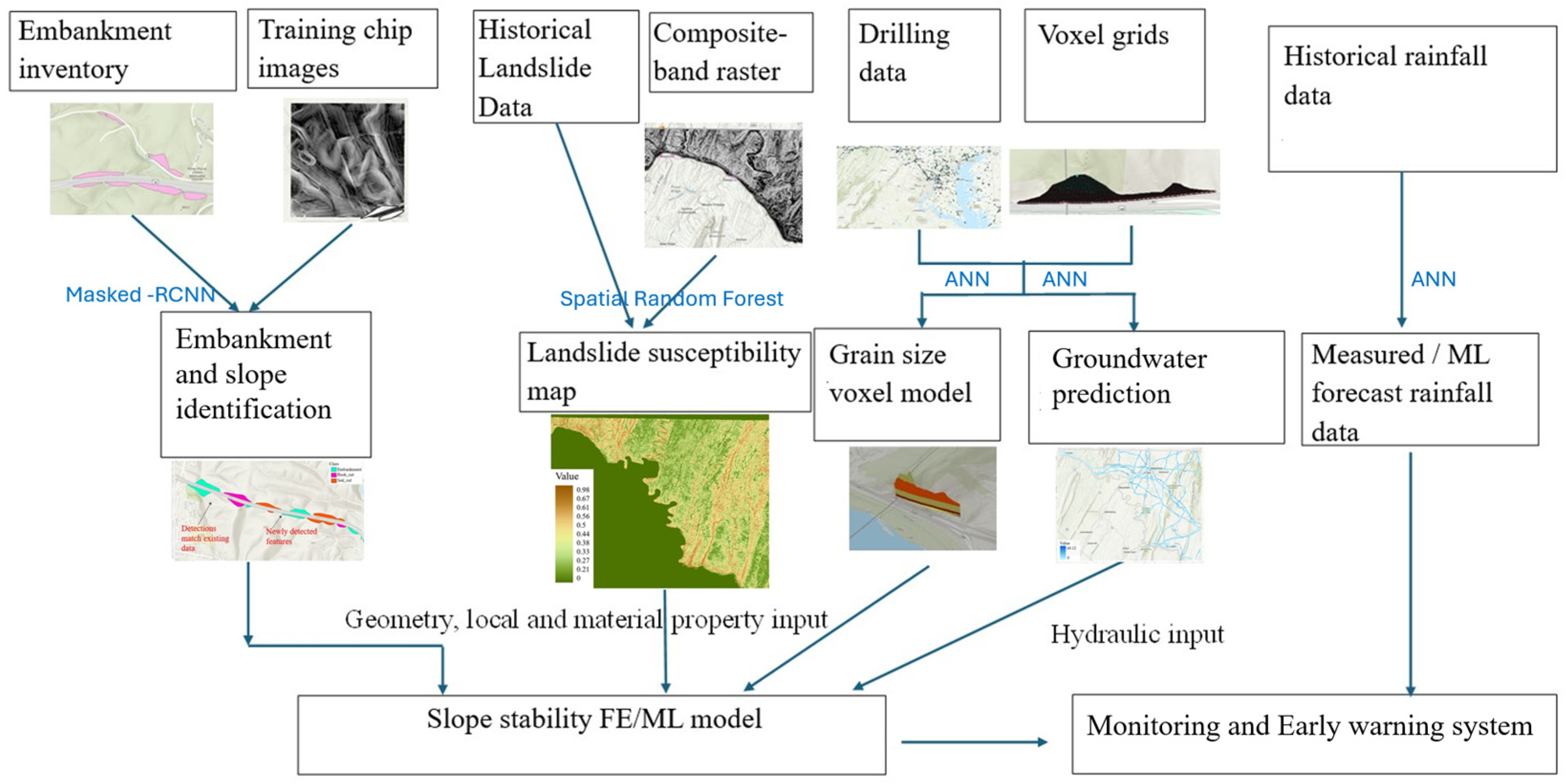Figure 1 illustrates the proposed digital twin framework. By training a random forest model, a statewide landslide susceptibility map was generated based on pixel-level predictions. Instance segmentation-detected polygons with high-landslide-risk scores are selected from the digital slope asset inventory to build a 3D subsurface voxel model, which has features of Unified Soil Classification System (USCS) soil type and groundwater depth. Using the provided geometry, initial material properties, and hydraulic inputs, a 3D finite element model can be developed to conduct seepage and slope stability analyses for selected slopes identified as high-risk areas. The time-varying FoS and failure probability analysis can be calculated with precipitation forecast data. The proposed digital twin methodology can be integrated with a highway asset management system for slope stability monitoring and emergency response.

The framework applied a 2D FEM analysis for slope stability. Two-dimensional finite element models are widely used for computation efficiency. These models assume the slope is uniform along one axis, which is good for consistent geometry and material properties. This model aims to be employed in large-area risk monitoring and early planning and design stages, where quick and reliable estimations of the factor of safety are needed without the heavy computational demands of 3D modeling [37] (pp. 653–654). However, 2D or 3D FE models are generally considered as computationally intensive. Surrogate modeling techniques such as machine learning models could provide more effective tools to alleviate computational demands. For example, such machine learning models can be trained with big datasets generated from many FE models or field measurement data. The framework is designed to identify high-risk locations across a large region or highway network. Therefore, quick and efficient evaluation is necessary, as there might exist a fairly large number of high-risk slopes in certain areas. In this case, a reduced dimensionality geotechnical model such as simple analytical predictions would be useful.

2.1. Creating Digital Slope Asset Inventory Using Machine Learning Techniques

A digital twin model for a regional-scale highway system requires a digital slope asset inventory to first be established, followed by populating feature values for numerical simulation models either through field investigation or machine learning prediction. Given the extent of highway networks and the complexity of terrain, there is a critical need for automated solutions that can efficiently and accurately detect and classify embankments and slopes. By employing instance segmentation techniques, 3D digital slope datasets including geometry and locations are first established in a commercial GIS software—Arc GIS pro 3.2.0 (2023) [38]. The model continuously integrates data from various sources, providing predictive insights and supporting asset owners with optimizing maintenance strategies, prioritizing interventions, and improving overall roadway safety and efficiency. Traditional methods for identifying and monitoring highway embankments and slopes often involve manual inspections, which are time-consuming in field survey and data gathering, labor-intensive in labeling and marking slope polygons, and prone to human error. The proposed approach seamlessly bridges the gap between physical infrastructure and its digital counterpart, providing a proactive, data-driven solution for efficient and sustainable infrastructure management.

The methodology employed in this research involves several key steps: data preparation, model development, training and validation, data augmentation, post-processing, and result analysis. Data exploratory analysis and pre-processing are a critical step in any machine learning task. In this study, 2 m resolution LiDAR DEM data were used as the primary dataset for slope detection. The 2 m resolution data were selected as they offer an optimal balance between capturing sufficient detail to accurately identify slope features and ensuring manageable data sizes for efficient computation. The LiDAR data were first pre-processed to remove noise and ensure consistency across the dataset. This step involved standardizing the data formats and aligning the coordinate systems to match the spatial reference required for subsequent analysis in ArcGIS Pro.

The DEM data were subsequently processed to generate slope raster images, serving as critical inputs for the machine learning model. The slope raster calculates the maximum rate of elevation change between each cell and its neighboring cells, highlighting areas with specific elevation variations indicative of embankments and slopes.

The development of the machine learning model started with the creation of a robust training dataset. Polygons of highway embankments and slopes that are susceptible to landslide risk are applied as inputs to generate training chips. Those polygons are available in shapefiles, which can be imported into the GIS software package—ArcGIS Pro 3.2.0 [38]—to visualize their locations and elevation features. These polygons of highway slopes exclude any water area. These polygons were used as masks on the slope raster to generate the training chips. This initial dataset comprised 11,884 image chips, each measuring 256 × 256 pixels, representing a ground area of 512 m × 512 m at the 2 m resolution. The training chips were extracted from statewide slope raster images, ensuring that the dataset captured a diverse range of embankment and slope features for robust model training. The instance segmentation model was designed to classify three distinct categories: embankment, soil cut slope, and rock cut slope. Each category demanded a unique set of features for precise identification, which the model learned during the training process. To enhance the model’s feature extraction capabilities, a ResNet-50 backbone architecture was used. ResNet, short for Residual Networks, is known for its ability to train very deep networks while avoiding the vanishing gradient problem. The 50-layer ResNet architecture offered the depth and advanced feature extraction capabilities required to effectively detect and classify embankments, soil cut slopes, and rock cut slopes from the LiDAR DEM data.

During training, the model underwent multiple cycles of forward and backward propagation, where the weights of the neural network were updated to minimize the loss function. The loss function measures the difference between the predicted outputs and the actual labels of the training samples. In this study, a typical training cycle consisted of 20 to 30 epochs, with the batch size set to 8. An early stop strategy was applied to the training procedure where no improvement was observed in the last 10 epochs.

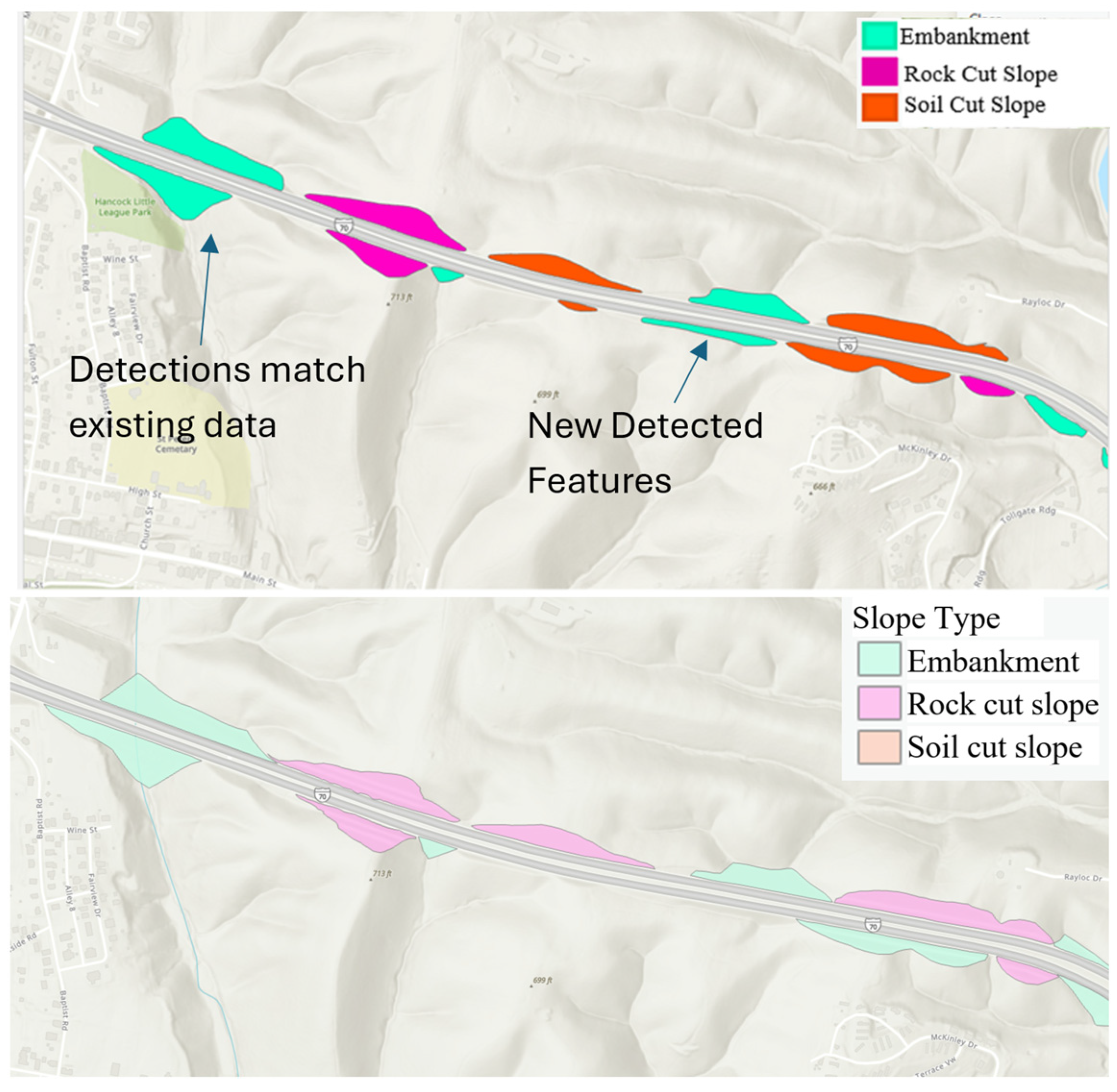
Post-processing is a critical step to enhance the quality and accuracy of the detected embankment polygons. Various techniques were employed to refine the model’s outputs and eliminate false positives or irrelevant polygons. This stage included using the Dissolve tool in ArcGIS Pro, which was instrumental in addressing overlapping polygons, filling voids and gaps, and separating individual components within multipart polygons. The tool also ensures the seamless connection of polygons representing the same embankment, thereby producing cohesive and accurate representations of the detected features. Quality control was an essential part of the post-processing phase. The detected polygons underwent several rounds of validation to ensure their accuracy and relevance, as shown in Figure 2, adjusting the model parameters, and refining the filtering criteria based on feedback from domain experts. This digital slope asset inventory dataset enhances transportation agencies’ ability to effectively monitor and manage their highway networks. By offering a more accurate and comprehensive view of embankments and slopes across the network, it supports proactive infrastructure management. Additionally, the automated detection and classification process significantly reduces the reliance on manual inspections, saving time and resources while improving data accuracy and consistency.

2.2. Identifying High-Risk Slopes from Regional Landslide Susceptibility Assessment

Landslides present substantial risks to transportation infrastructures, particularly road networks in geologically sensitive regions. This study developed a pixel-level geospatial machine learning model to assess landslide risk along a regional highway network, leveraging geospatial and geophysical features of specific locations. A random forest (RF) classification algorithm was utilized to predict the probabilistic occurrence of landslides, incorporating historical slope failure data alongside multiple terrain and environmental variables derived from LiDAR DEM data. The RF algorithm offers several advantages for predictive modeling: it is nonparametric, accommodates both categorical and continuous variables, and demonstrates robustness against correlated input features. Additionally, it can assess variable importance based on out-of-bag (OOB) data, providing insight into which factors are most influential in landslide prediction. The model’s flexibility and speed make it suitable for handling large geospatial datasets like those derived from LiDAR.

An approach to identify the slopes at the highest risk for digital twin model-based monitoring through a landslide susceptibility assessment was adapted from the work by Maxwell et al. (2020) [39]. The RF model predicts the probability of landslide occurrences by aggregating the votes of multiple decision trees, each constructed from randomly selected subsets of the training data. In this study, the RF model incorporates 35 features derived using Python v.3.10.9 scripts in ArcGIS Pro 3.2.0 [38] and R v.4.3.2 geospatial analysis packages. Key terrain variables used in the model are summarized in

Table 1. Input features used for landslide risk machine learning model.

Feature Category	Feature Name	Description
Terrain Features	Slope Gradient (slp)	Measures the steepness of the terrain.
	Slope Position (sp1, sp2, sp3)	Indicates the relative position of the slope in the landscape (averaged over different window sizes: 7 × 7, 11 × 11, 21 × 21).
	Topographic Roughness (tr1, tr2, tr3)	Captures the irregularity of the terrain, affecting stability (window sizes: 7 × 7, 11 × 11, 21 × 21).
	Topographic Dissection (td1, td2, td3)	Indicates the extent of terrain dissection (window sizes: 7 × 7, 11 × 11, 21 × 21).
	Mean Slope Gradient (slpmn1, slpmn2, slpmn3)	Average steepness across different window sizes (7 × 7, 11 × 11, 21 × 21).
	Site Exposure Index (sei)	Reflects the exposure of the terrain to environmental factors like wind and sunlight.
	Heat Load Index (hli)	Represents the effect of solar radiation on terrain, potentially influencing water retention and slope stability.
	Linear Aspect (LnAsp)	Describes the compass direction the slope faces.
	Surface Relief Ratio (srr1, srr2, srr3)	Measures the variation in elevation over a given area, affecting risk (window sizes: 7 × 7, 11 × 11, 21 × 21).
	Surface Area Ratio (sar)	Compares the surface area to horizontal area, highlighting areas prone to instability.
	Profile Curvature (prc1, prc2, prc3)	Describes the curvature of the terrain in the direction of the slope (window sizes: 7 × 7, 11 × 11, 21 × 21).
	Plan Curvature (Plc1, Plc2, Plc3)	Measures the curvature of the terrain along contour lines (window sizes: 7 × 7, 11 × 11, 21 × 21).
	Cross-Sectional Curvature (csc1, csc2, csc3)	Reflects curvature perpendicular to the slope, affecting water runoff and erosion (window sizes: 7 × 7, 11 × 11, 21 × 21).
	Longitudinal Curvature (LnC)	Describes the curvature of the terrain along the direction of water flow.
Non-Terrain Features	Lithology (lith)	Represents different rock types, with 34 categories present in Maryland, influencing slope stability.
	Distance to Nearest Road (USD)	Measures the proximity to roads, accounting for the impact of construction on slope stability.
	Cost Distance to Streams (StrmC)	Represents the effort for water to reach streams, reflecting areas prone to slope saturation.

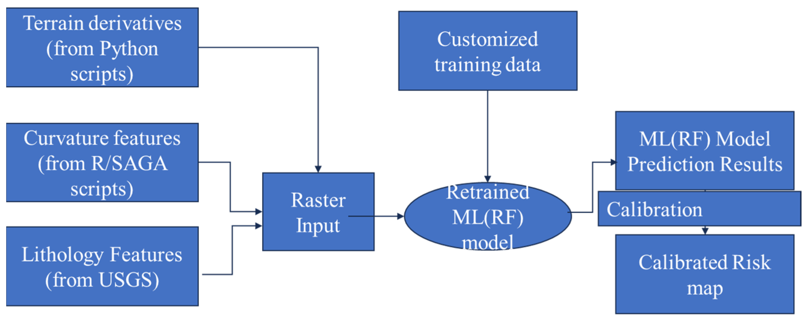
. Each variable was computed across multiple window sizes to account for terrain variations at different spatial scales, enhancing the model’s ability to capture nuanced geophysical patterns associated with landslide risk. Figure 3 shows the framework of generating the ML-based landslide susceptibility map, and the structure of the RF classification model applied in the framework is shown in Figure 4. The trained RF model generates probabilistic landslide susceptibility values for regions with feature characteristics similar to the training data. The resulting landslide risk map serves as a valuable resource for engineers and policymakers, enabling the identification of high-risk areas and guiding the implementation of preventive measures. Figure 5 showcases a sample landslide susceptibility map located near Washington county, Maryland, which was produced by the RF model, with areas of elevated landslide risk highlighted in deep red. Locations scoring above 0.7 on the risk scale were flagged for further investigation. After calculating landslide risk scores with the RF model, these scores were integrated with the digital slope asset inventory derived from the previously described instance segmentation method. A spatial statistical analysis was conducted to compute the average landslide risk score for each slope polygon. Polygons identified as having high landslide risk were prioritized for further actions, such as the development of digital twin models and real-time monitoring systems.

2.3. Digital Twin Platform for Slope Instability Monitoring

The proposed digital twin platform utilizes AI-generated data to create numerical models for short-term slope stability monitoring and prediction, incorporating near-future precipitation forecasts. Slopes identified with high landslide risk in the previously developed digital slope asset inventory are selected for detailed analysis. A 3D subsurface voxel model is constructed for each of these slopes, with feature values such as USCS soil type and groundwater depth populated using machine learning model predictions.

Subsequently, a 3D finite element model is developed for the selected slopes to perform seepage and slope stability analyses under forecasted precipitation conditions. This approach enables the computation of time-varying factors of safety and failure probabilities, which can be exported from the finite element model for further evaluation and decision making.

2.3.1. Machine Learning Model for Groundwater Depth

This study utilizes a groundwater depth dataset comprising 4930 samples from 4476 boreholes distributed along the Maryland state road network. To enhance the dataset, a surface water point dataset was appended, containing 2700 samples from locations along the coastlines of water bodies. These surface water points serve as control points with zero groundwater depth, enriching the training dataset and improving model accuracy. Space features of these data points include their GPS coordinates (latitude, longitude) and elevation, which were computed from LiDAR DEM data. An average slope raster was calculated from 2 m resolution LiDAR DEM using a 3 × 3 moving window. Additionally, a 12-digit watershed code and distance to the nearest watershed boundaries were also used as input features for machine learning model training. Watershed boundaries represent approximate lines of surface water divide, where water begins to flow toward rivers through the interior portions of each watershed. These boundaries are valuable for training purposes, as groundwater generally flows inward from these divisions, providing an important context for understanding subsurface hydrological patterns.

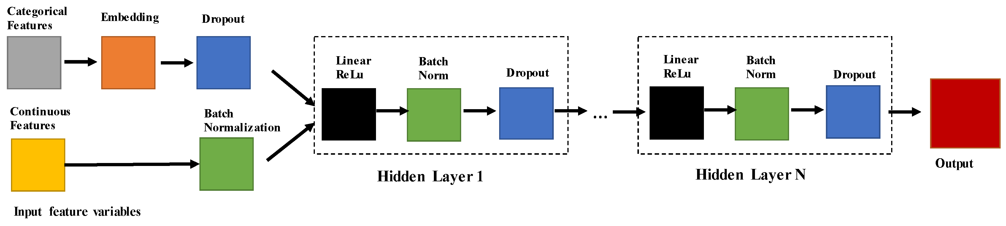
A 2-layer artificial ANN regression model for tabular data was adopted in this study. For the groundwater depth ANN model, an embedding layer was applied to convert categorical feature variables into a form compatible with the neural network, which, along with other numerical features, served as input to the first layer. The structure of the ANN model is shown in Figure 6. Based on findings from a parametric study of various input feature variables, the categorical variables were selected as drilling month, soil type in the format of United States Department of Agriculture Soil Survey Geographic Database (USDA SSURGO) map unit symbol (MUKEY), and 12-digit Maryland watershed code. The numerical feature variables included latitude, longitude, surface elevation, average slope, and distance to the nearest waterbody. A parametric study was conducted to identify the optimal number of layers and neurons, resulting in the selection of a 2 × 200 neural network for the hidden layers. The output layer produces predicted groundwater depth based on given input feature variables. A data resample strategy was applied on the training data to overcome the data imbalance issue where samples from the minority group were underrepresented for ML model training. An oversampling strategy that increases the weights of minority group data was employed to enhance the performance of groundwater depth ML model. The combination of oversample factors, as listed in

Table 2. Oversampling factor values for different bucket ranges.

Groundwater Depth Range (Unit: 0.3048 m)	Oversample Factor
[0, 8]	6
[8, 12]	10
[12, 16]	10
[16, 28]	10
[28, 52]	12
>52	16

, for the model was then determined after parametric study. For the groundwater depth model training, 90% of the dataset was randomly allocated for training, with the remaining 10% used for validation. The Rectified Linear Unit (ReLU) was used as an activation function for hidden layers. For this regression problem, the mean square error (MSE) loss function was used. The learning rate (LR) for training was 0.001, which was determined from the LR–loss plot. The model was trained by 200 epochs with a batch size of 2048. The model converged after 118 epochs of training. At the end of 200 epochs, the training loss and validation loss were 9.165 and 9.517. The validation set reached an RMSE of 3.085. The training and validation loss curves are shown in Figure 7.

After training, the model’s predictive accuracy was evaluated through a test on unseen data, comparing its predictions against actual values obtained from field investigations. The model demonstrated strong performance, achieving an overall Root Mean Square Error (RMSE) of 2.317.

The machine learning model was applied to predict the groundwater depth for a 210 m wide buffer zone along the highway route network in a selected region, as shown in Figure 8. A 20 m spacing grid was generated within the buffer zone using data extracted from the LiDAR DEM. This grid captures detailed geophysical information, and grid points located inside the boundaries of detected embankments and slopes were used as geometry and material input, ensuring comprehensive spatial coverage for analysis. Geospatial and geological parameters for these grid points were calculated and appended to the shapefile, ensuring each grid point contained comprehensive attribute data for machine learning prediction. Monthly groundwater depth predictions were subsequently generated using the machine learning model optimized for production deployment. The yearly median and the range (difference between maximum and minimum values) of groundwater depth were computed and converted into a 20 m resolution raster file for spatial analysis. Figure 8 presents a generated groundwater depth map, where lighter shades of blue indicate shallower groundwater depths, and darker shades represent deeper levels, effectively illustrating the spatial variation in groundwater distribution. The predicted groundwater depth ranges from 0 to 75 ft. Figure 9 shows a groundwater table elevation map using machine learning-predicted values. The median value was then added to the embankment and slope inventory shapefile, providing an estimation of the initial groundwater conditions for use in the digital twin model for slope stability analysis.

2.3.2. Machine Learning Model for USCS

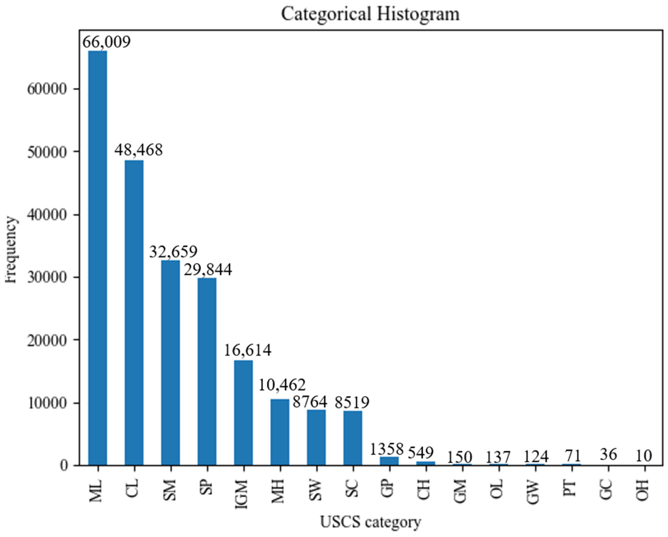
The digital twin model for slope stability analysis relies on input data detailing soil types and their corresponding parameters. To address this need, machine learning models have been developed to estimate soil types and parameters for specific locations. Previous studies have demonstrated the effectiveness of machine learning in predicting soil properties [40,41]. In this study, tabular drilling data were utilized to train an ANN model for predicting soil types consistent with USCS. The predicted soil parameters serve as critical inputs for time–history finite element analysis of slope stability models. The USCS soil type drilling dataset consists of 212,633 samples collected from 10,349 boreholes across the Maryland state road network. These samples were taken at 1 ft intervals, with labels indicating the USCS soil type at the bottom of each 1 ft layer. The model includes all layers above the bedrock, covering 15 different USCS soil classes and Intermediate Geomaterials (IGMs). The histogram in Figure 10 illustrates the distribution of soil types, with inorganic sand, silt, and clay with liquid limits under 50% (ML, CL) being the most common, with over 60,000 and 40,000 samples, respectively. Conversely, peat (PT), clayey gravels (GC), and organic clays (OH) are the least represented soil types in the dataset, with fewer than 100 samples each. This imbalance can bias the model, as minority classes may be underrepresented. To address this, a data oversampling strategy was employed, applying varying oversampling factors to enhance the representation of minority classes, as shown in

Table 3. Oversampling factor values for USCS soil type dataset.

USCS Label	Oversample Factor
ML	2
CL	3
SM, SP	3
IGM	5
MH, SC, SW	7
GP, CH, GM, OL, GW, PT, GC, OH	25

. The most effective combination was identified and utilized for model training, ensuring a more balanced and robust prediction performance.

Feature engineering played a key role in transforming the raw data to capture the underlying patterns more effectively. An iterative wrapper feature selection method was employed, systematically evaluating and selecting the most relevant features to optimize the model’s performance. The ANN models were trained using features such as spatial coordinates, surface elevation, drilling depth, and soil parent material.

A 4-layer ANN model for classification was employed in this study. For the grainsize prediction model, an embedding layer was applied to transform the soil parent material categories into a format suitable for neural network processing. This embedding, along with four other numerical features, was used as input to the first layer. The output layer generates confidence scores for each grain size category, with the final prediction based on the category with the highest confidence score. The Rectified Linear Unit (ReLU) was used as an activation function for hidden layers, for its simplicity and efficiency. It helps the neural networks learn complex patterns by introducing non-linearity while also reducing overfitting by deactivating certain neurons. For this multi-classification problem, the categorical cross-entropy loss function was used. The learning rate (LR) for training was 0.001, which was determined from the LR–loss plot, at the point where the loss decreases the most before increasing again.

For the USCS soil type (grain size) model training, 90% of the dataset was randomly allocated for training, with the remaining 10% used for validation. The model was trained by 600 epochs with a batch size of 10,384. The model converged at the end of 600 epochs, and the training loss and validation loss were 0.486 and 0.471. The training loss curve is shown in Figure 11. The validation set reached an accuracy score of 0.804. The accuracy report for the model, trained using the most effective oversampling factors, is detailed in

Table 4. Accuracy report for the grain size machine learning dataset.

Category	Precision	Recall	F1-Score	Support
CH	0.43	0.99	0.6	549
CL	0.84	0.82	0.83	48,468
GC	0.35	1	0.52	36
GM	0.35	0.99	0.51	150
GP	0.37	0.99	0.54	1358
GW	0.37	0.95	0.53	124
IGM	0.75	0.92	0.83	16,614
MH	0.6	0.9	0.72	10,462
ML	0.91	0.71	0.8	66,009
OH	0.91	1	0.95	10
OL	0.66	1	0.8	137
PT	0.57	1	0.72	71
SC	0.53	0.8	0.64	8519
SM	0.78	0.69	0.73	32,659
SP	0.81	0.73	0.77	29,844
SW	0.55	0.82	0.66	8764
Accuracy			0.77	223,774
macro-avg	0.61	0.9	0.7	223,774
weighted-avg	0.8	0.77	0.78	223,774

. In this report, the accuracy refers to the proportion of correctly classified instances (both positive and negative) relative to the total number of instances, which is a general indicator of how often the model is correct. Precision quantifies the proportion of true positive predictions among all instances predicted as positive, which focuses on the reliability of positive predictions.

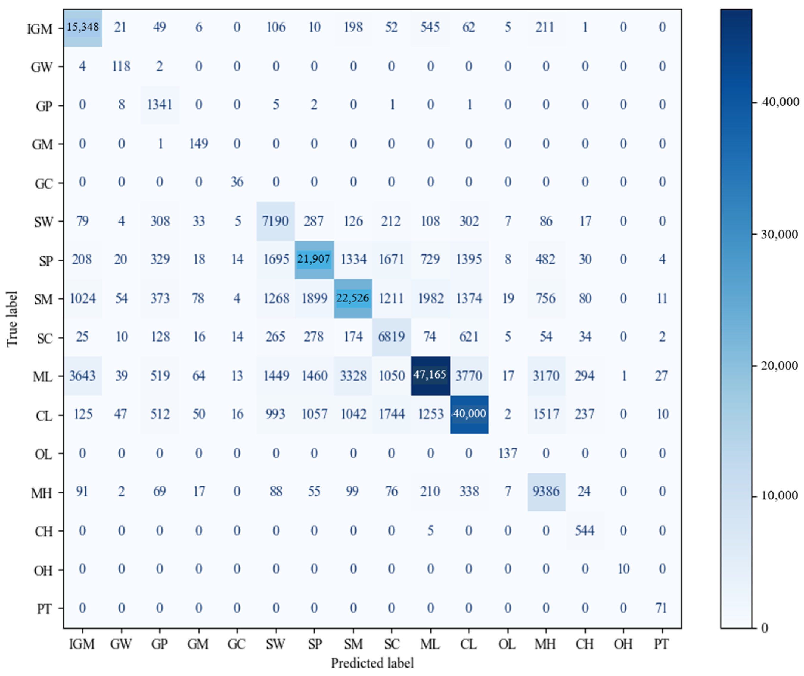
The model achieved an overall accuracy of 0.77, with F1-scores for individual categories ranging from 0.55 to 0.95. A confusion matrix heat map (shown in Figure 12) was generated to evaluate the classifier’s performance in the multiclass classification task, providing a clear visual representation of the true versus predicted classifications for each soil type. Correctly classified instances are located along the diagonal, while those misclassified instances are represented by the off-diagonal elements. In this study, the soil type labels were arranged by grain size and liquid limit, organized in the order of IGM, gravel, sand, silt, and clay. The confusion matrix shows the highest counts along the diagonal, with elevated counts near the diagonal, indicating the model’s strong performance in classifying similar soil types.

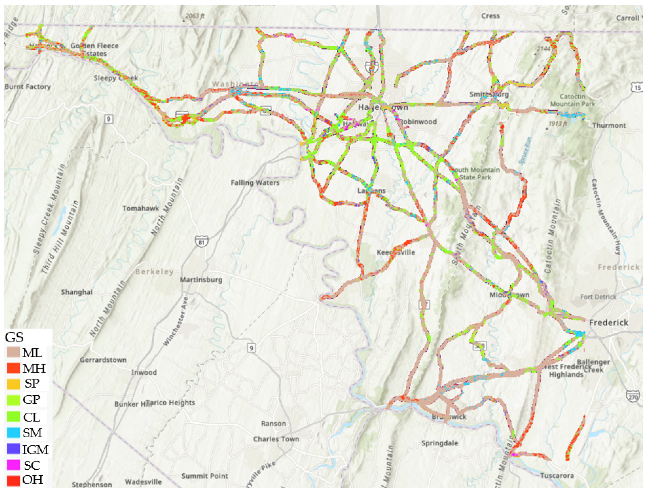
Once the model was trained, a soil type map using the predicted values can be generated for grid points with the selected highway buffer zone. Figure 13 presents the prediction results at a depth of 1.5 m (5 feet) within the highway buffer zone, showcasing the model’s capability to classify soil types accurately at this depth. Furthermore, the model can be extended to generate a 3D soil property network, as illustrated in Figure 14. This analysis underscores the model’s effectiveness in detecting subsurface heterogeneities, which are vital for assessing slope stability, especially in landslide-prone regions.

3. Case Study: Demonstrating Short-Term Slope Stability Prediction Using FEM Analysis and Forecasted Precipitation Data

This case study demonstrates the application of a digital twin platform, integrating finite element (FE) simulation with forecasted precipitation data, for short-term slope stability monitoring. The approach highlights the potential for proactive slope monitoring and risk management, particularly for areas prone to instability during extreme weather events. In advanced engineering projects, finite element modeling (FEM) often serves as a core component in the digital twin model. By leveraging detailed FEM simulations, digital twins can quantitatively model infrastructure response behavior and dynamically adapt to changing conditions in real time by integrating monitoring data feeds. Machine learning model-predicted values can be potentially used for providing input feature values of the digital twin model if field investigation is insufficient or unavailable, enabling efficient seepage and slope stability analyses. This approach helps fill data gaps and supports accurate modeling in the absence of comprehensive on-site measurements.

For demonstration purposes and due to computing resource constraints, a 2D finite element model was developed to serve as the physical twin counterpart within the digital twin framework. This model effectively showcases the integration of predictive modeling and simulation, enabling enhanced decision making by providing valuable insights into seepage and slope stability under various conditions. Seepage analysis aims to understand groundwater movement through soil, which significantly affects pore water pressure and, consequently, slope stability. FEM enables detailed simulations of steady-state or transient seepage under variable conditions, such as rainfall or water table fluctuations, by discretizing the soil into finite elements and solving pore pressure and hydraulic gradients. Slope stability analysis, on the other hand, often relies on the limit equilibrium method (LEM), which assumes a potential failure surface and analyzes the forces or moments acting on the soil mass to compute the FoS. Techniques like Bishop’s Simplified Method, Janbu’s Method, and the Morgenstern–Price Method are commonly used to handle circular and non-circular slip surfaces, accommodating varying geometries and loading conditions. These methods are implemented in software tools such as SLOPE/W module in GeoStudio 2023.1.1, allowing for stability assessments under seismic loads or fluctuating water levels.

Seepage and slope stability analyses are often interdependent, especially in scenarios where dynamic groundwater conditions, such as rapid drawdown or intense rainfall, significantly influence slope stability over time. Coupled seepage–stability analysis enables engineers to evaluate how transient changes in pore water pressure impact slope behavior, ensuring that designs remain robust under both steady-state and dynamic conditions.

The FE model serves as a virtual surrogate for the physical twin in the digital twin framework. A 2D FE model was developed using a software package, MIDAS GTX NS v1.1 [42], in order to demonstrate slope stability monitoring under rainfall conditions. The study area is near Fort Washington, Maryland. The slope model parameters considered for the model include surface elevation, geometry, material properties, soil layer distribution, and groundwater depth. A real precipitation dataset from 2–5 May 2014, when a historical landslide event occurred in the study area, was utilized to model the surface water flux input to the site. The analysis was segmented into stages based on precipitation rates. Each stage comprised three components: a transient seepage analysis, an in situ initial condition stress–strain analysis, and a slope stability analysis employing the strength reduction method. Seepage analysis works as parent analysis for the stress–strain analysis. The output from this semi-coupled finite element model includes stress–strain distribution contour plots, which can be used to estimate the starting point of sliding surface. The time–history response of displacement at various stages will be presented to visualize the progression toward failure and pinpoint the failure time. Additionally, the deterioration curve of the strength reduction factor will be provided to illustrate the reduction in slope stability leading up to failure.

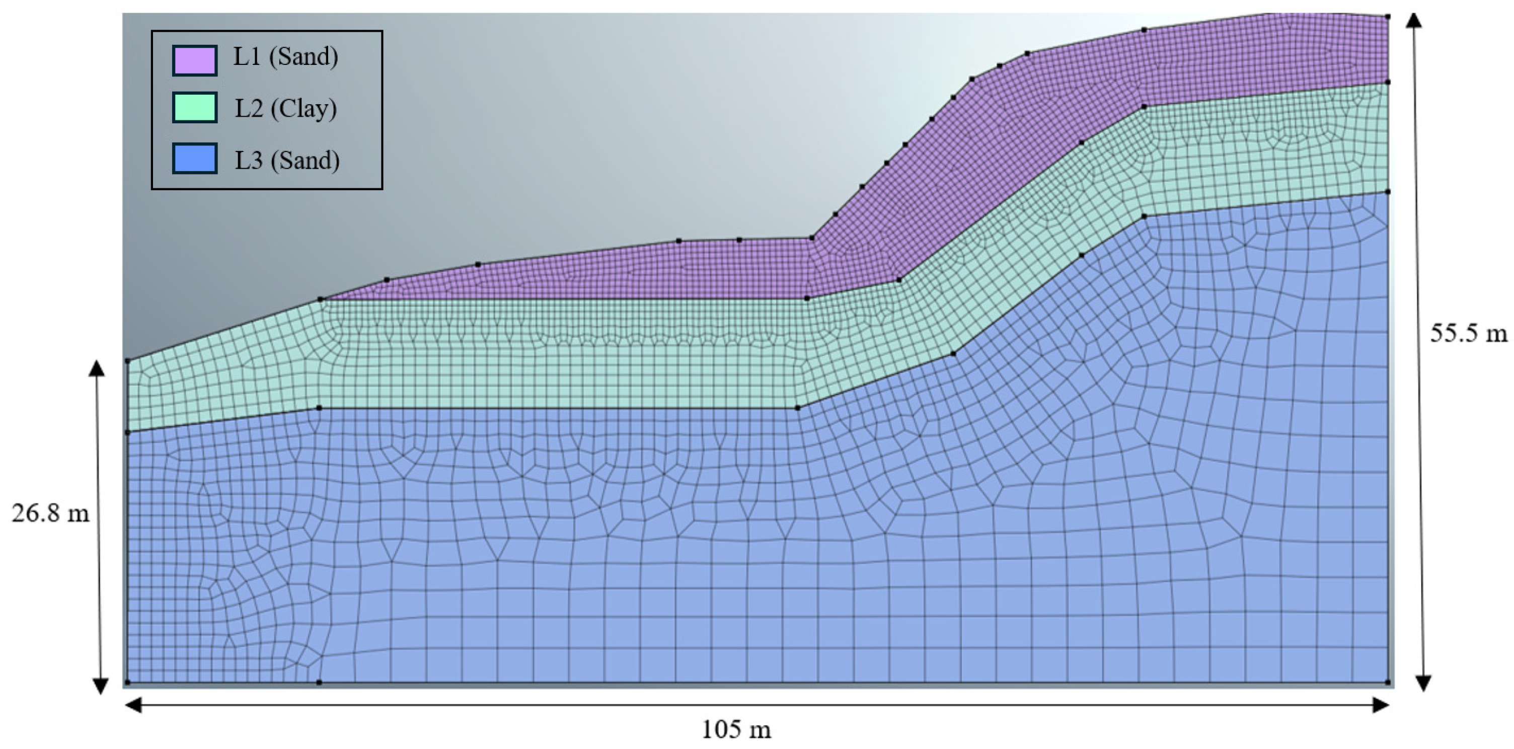
The geometric layout and mesh of the 2D FE model is depicted in Figure 15, with a horizontal dimension of 105 m and a vertical height of 55.5 m. The field test borings and CPT data revealed a soil profile consisting of three distinct strata, consistent with published geological data. According to a field investigation report by KCI (2014) [43], Stratum I (Nangemoy Formation, Ta) primarily comprises moist to wet, brown to dark gray, very loose to medium-dense silty sand, clayey sand, and sand with gravels, interbedded with soft to stiff layers of sandy silt and sandy clay. Below this, a 20–30 ft thick layer of Stratum II (Marlboro Clay, Tm) is present, consisting of moist to wet, reddish-brown to light gray lean clay with occasional thin lenses of micaceous silt. In some localized areas, fat clays were also encountered. Beneath the Marlboro Clay lies Stratum III (Aquia Formation, Ta), consisting of moist to wet, olive gray to dark gray silty sand and sandy silt, with scattered mica and calcareous shell fragments throughout the stratum. The geometric boundary lines of the 2D FE model were drawn using field test data, as shown in Figure 15. The Mohr–Coulomb constitutive model has been chosen to represent soil materials in this model. The detailed physical and mechanical properties of the soil materials are provided in

Table 5. Physical parameters of slope finite element model in the case study.

	L1 (Sand)	L2 (Clay)	L3 (Sand)
Elastic modulus (N/m2)	2.5 × 107	7 × 106	2.3 × 107
Poisson’s ratio (v)	0.25	0.3	0.25
Unit weight (N/m3)	18,630	18,060	18,630
Cohesion (N/m2)	20,000	5 × 104	5.2 × 104
Friction angle (degree)	25	30	32

.

4. Analysis and Discussions

This section demonstrates how the integration of the FE model with forecasted precipitation data within a digital twin framework can facilitate slope stability monitoring and near-future landslide risk assessment. Specifically, the 2D FE model is utilized to compute the time-dependent variation in the FoS, accounting for the impact of rainwater infiltration and the progression of wetting fronts on slope stability. The model simulates the slope displacement from the start of the rainfall event to the landslide-triggering point. Rainwater infiltration into the subsurface can result in the formation of perched water tables and an elevation in the main groundwater level. Precipitation is a proxy for soil moisture, which is usually gauged by looking at precipitation in a period leading up to the slide (antecedent moisture) and intensity of rainfall in a shorter period immediately preceding the slide. Rainfall intensity, cumulative precipitation, and the timing of rainfall all have a role in slope failure. Accurate long-term global precipitation estimates, especially for heavy precipitation rates, at fine spatial and temporal resolutions are thus vital for slope instability studies and early warning systems with appropriately defined rainfall threshold values. Satellite-based precipitation products provide both spatially and temporally continuous observation data to determine the areal precipitation distribution compared with ground-based station data. The active publication of several precipitation-based datasets presents an opportunity for integration with spatial LiDAR terrain data, and subsurface soil mapping for slope instability prediction applications. Some of the satellite-based precipitation products used today are as follows: tropical rainfall measuring mission (TRMM) and Integrated Multi-Satellite Retrievals for Global Precipitation Measurement (GPM-IMERG). The GPM data are presently published by NASA, which are used to map landslides globally.

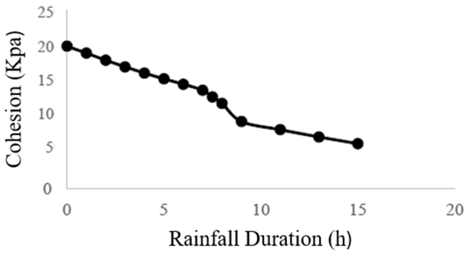
The hydrological changes in the slope can increase pore water pressure and decrease soil matric suction. Together, these effects lead to a reduction in the shear strength of the soil along potential failure planes. When the shear strength diminishes below a critical threshold, slope instability and eventual failure become imminent. The physical parameters of each layer are summarized in Table 5. All soil layers were considered as isotropic Mohr–Coulomb material, where the cohesion and internal friction angle are the two key parameters for slope stability analysis. This study utilized a regression model to analyze the impact of increased moisture content on soil mechanical properties. The adjusted deterioration curve for the cohesion of layer 1 is visualized in Figure 16.

The permeability and water-bearing functions are given as Equations (1) to (3) below, while the coefficients and their values used for the function are described in

Table 6. Hydraulic parameters of slope finite element model in the case study.

Layer	Stratum	Description	a (pa)	n	M	Ks (m/s)
1	SM, SC, SP	Silty sand, clayed sand, coarse sand	8.50 × 102	2.1	0.52381	8.25 × 10−3
2	CL, CH	Lean clay, fat clay	1.22 × 104	1.2	0.166667	5.55 × 10−5
3	SM, ML	Silty sand, sandy silt	1.00 × 103	1.9	0.473684	9.80 × 10−3

, adapted from previous laboratory test results [44,45]. The curves for the permeability K ratio and water content curve with respect to pore pressure are shown in Figure 17. The hydraulic boundary for the seepage was defined by the groundwater depth and water flux from rainfall infiltration. The groundwater depth in this study is taken as 25.5 m from the top point of the slope, where the hydraulic nodal head of the slope bottom is 30 m. The surface water flux was determined by the daily precipitation data downloaded from the NOAA National Weather Service’s Precipitation Frequency Data Server. This study only considered the first two stages of precipitation data input, as shown in Figure 18 The x axis refers to the duration of precipitation in hours and the y axis refers to the precipitation rate. For this analysis, the pressure head was set to zero using a node head operation. The entire slope surface of the model was designated as the rainfall infiltration surface, simulating a short-term heavy rainfall condition that lasted 8 h. A water flux boundary condition was applied to the top edge of 2D model as listed in

Table 7. Water flux input.

Stage	Water Flux (in/h)	Water Flux (m/s)	Duration (h)
1	0.08	5.64 × 107	7
2	0.17	1.20 × 10−6	2

. The definitions of variable to calculate permeability function in Equation (1) to (3) are listed in

Table 8. Abbreviation definition and unit.

Parameters	Definition	Unit
${\theta }_r$	soil residual volume water content	-
${\theta }_s$	saturated volume water content	-
$m$	empirical fitting parameter	-
$n$	empirical fitting parameter	-
$a$	empirical fitting parameter	pa
Ks	saturated permeability	m/s
h	pressure head	M

.

$$\theta ={\theta }_r+{\displaystyle \frac{{\theta }_s-{\theta }_r}{{{[1+(a\times h)}^n]}^m}},$$

(1)

$$m=1-{\displaystyle \frac{1}{n}},$$

(2)

$$K={\displaystyle \frac{{\theta }_W-{\theta }_r}{{\theta }_s-{\theta }_r}}$$

(3)

In the subsequent stress model, boundary conditions were defined with the bottom boundary fixed, and the left and right edges restricted in the y-direction. The finite element mesh size was configured at 0.5 m for the first layer to capture finer details, and 2 m for the second and third layers to maintain computational efficiency. The following criteria were applied in the finite element model for the strength reduction analysis: The plastic zone of the slip surface becomes fully connected. Displacement and strain on the slip surface experience abrupt changes, resulting in significant and unbounded plastic flow; a dual convergence criterion based on both stress and displacement was used; if the model fails to converge when evaluated by these criteria, it indicates that slope failure has occurred. The model includes a transient seepage analysis for a duration of 8 h, and nine discrete stress strength reduction method (SRM) analyses with 1 h intervals.

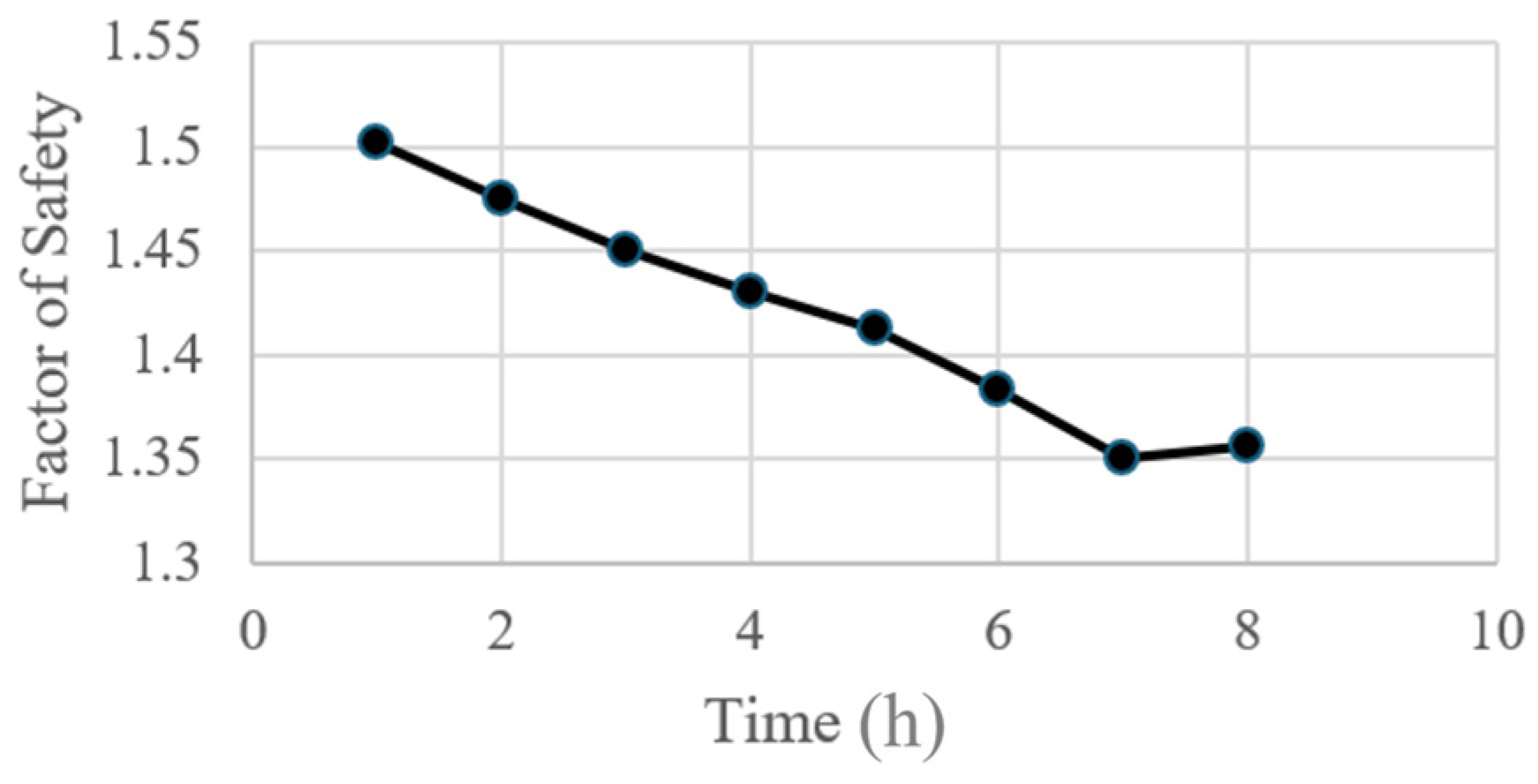
To calculate the safety and stability coefficients of the slope model under rainfall infiltration, an SRM analysis was conducted at each 1 h time step. The FoS value was determined by analyzing the safety factor versus maximum displacement curve, which was plotted when non-convergence was observed in the solution. Figure 19a shows the FoS value over the time duration of 2 h is 1.475, while the slip surface is not penetrated. As shown in Figure 20, according to the displacement contour plot for the slope, the displacement at the foot toe of the slope has the largest value, where the maximum displacement reached 1.531 mm. Figure 19b shows the FoS value during the time duration of 8 h, which demonstrates a decreasing trend of FoS from 1.43 to 1.356. Figure 21 shows the time–history curve of the slope FoS, which decreased from 1.50 to 1.326 over this eight-hour period. In general, rainfall infiltration substantially impacts the deformation of soil masses, which in turn affects slope stability. The numerical simulation results also provide the critical rainfall threshold values for slope failures that can be set based on precipitation-related indices along with geological, morphological, and hydrological conditions for the considered slope. Therefore, the effects of rainfall should be considered in any landslide early warning system. The proposed digital twin model for highway slope stability monitoring should thus consist of four elements: precipitation data on a near-real-time basis and forecasted precipitation in the next few days, risk knowledge of the slopes located within the considered highway network system, monitoring and quantitative analysis models, which relate excessive precipitation with slope instability sensitivity, dissemination, and a slope inspection notification system, and real-time recording of the event information and corresponding slope condition variation during storm events. To avoid computationally demanding 3D FE simulation, a machine learning surrogate model can also be trained and utilized to compute landslide rainfall thresholds once many numerical simulations across various slopes in the highway system have been completed to generate the necessary training data.

5. Discussions

To address the requirements of regional-scale highway slope stability risk monitoring and early warning systems, this study proposed an AI-powered digital twin framework. This digital twin platform integrates LiDAR-derived DEM data and instance segmentation methods to create a comprehensive digital slope asset inventory for a regional highway network. Furthermore, AI-generated data are employed to develop numerical simulation models, such as finite element models, enabling short-term slope stability monitoring and prediction based on near-future forecasted precipitation data. The findings of this study highlight several critical contributions to advancing infrastructure resilience and management with emerging machine learning and digital twin technologies.

1.

Automated generation of digital embankments and slopes inventory at a regional scale: By leveraging high-resolution LiDAR data, the digital twin framework utilizes a digital slope asset inventory efficiently detected by AI algorithms for embankments and slopes across regional highway networks with a minimum elevation difference (highest point and lowest point of the slope) of 15 ft for the slope. The instance segmentation model offers automated detection capabilities that significantly reduce reliance on manual inspection and marking. This automation not only saves time and resources but also enhances detection accuracy. These advantages make the model particularly valuable for creating a regional-scale geotechnical asset inventory, streamlining the process of cataloging and managing geotechnical assets at a regional scale.

2.

Applying machine learning for regional landslide risk assessment: The digital twin framework incorporates random forest and ANN models trained on historical data, to enable the prediction of the landslide susceptibility score and key subsurface features, such as soil type and groundwater depth. It should be noted that training data quality assurance is important for the ML model development. There should be enough training data near the site of 3D subsurface voxel model, and care should be excised for construction project sites with excavation work completed after the training dataset was collected. The training dataset needs to be regularly updated as new borehole data from recent subsurface exploration projects become available. Historical data features, such as GPS coordinates collected 20 years ago, do not have the same level of accuracy as modern data. Additionally, an oversampling scheme requires careful execution and validation to avoid hallucination in predictions. Potential mitigation strategies such as ensemble methods can be incorporated into future study.

3.

This predictive capability allows for near-real-time slope stability monitoring with a numerical simulation model established for those slopes with higher landslide risks in the highway system.

4.

Automated generation of slope physical parameters for stability analysis: The digital twin platform facilitates slope stability assessment by providing a 3D subsurface voxel model filled with AI-generated soil properties and groundwater depth values for selected sites. Machine learning model-predicted values can potentially be used for providing input feature values of the digital twin model if field investigation is insufficient or unavailable, enabling efficient seepage and slope stability analyses. This approach helps fill data gaps and supports accurate modeling in the absence of comprehensive on-site measurements.

5.

Early warning system for slope failures: By integrating time-dependent environmental variables, such as forecasted precipitation data retrieved from online databases, the digital twin framework can serve as an early warning system for short-term slope stability monitoring and emergency response. The system’s ability to simulate slope response behavior over time is invaluable for maintaining resilience in highway networks.

6.

Scalability and extension to other applications such as resilient hillside communities to climate change and extreme weather events: The proposed digital twin framework is adaptable to diverse geographic and geotechnical settings, making it scalable for broader use in infrastructure management. Climate change is expected to significantly impact slope stability by altering precipitation patterns, primarily through increased intensity and frequency of heavy rainfall events, which can lead to higher water infiltration into slopes. There is a growing need for landslide risk monitoring for areas that have not been identified before. When integrated into GIS platforms such as ArcGIS Pro 3.2.0, the digital twin model can become an active component of transportation management systems, providing ongoing updates and risk mitigation strategies for state and federal transportation agencies. The toolbox in ArcGIS Pro can be customized to meet the specific requirements of users. Machine learning packages can now be embedded in ArcGIS Pro 3.2.0 [38] to train ML models and make predictions tailored to users’ needs. There is a growing trend to explore the interaction between FEM software and the GIS platform (ArcGIS Pro 3.2.0. For example, FEM mesh (nodes, elements) can be exported from geospatially referenced formats (e.g., shapefiles, GeoJSON, or CSV) directly from ArcGIS Pro 3.2.0, while FEM simulation results can be visualized and stored in geospatially referenced formats for further analysis in ArcGIS Pro 3.2.0.

6. Conclusions

This research demonstrates the feasibility of digital twins in slope stability monitoring; however, further enhancement, such as incorporating real-time hydrology monitoring data for more dynamic, adaptive risk management, is still needed. Additionally, 3D FE simulations are computationally intensive, particularly when used to calculate the transient response of slope displacement and FoS. Machine learning surrogate models can be developed to compute landslide rainfall thresholds and predict slope response to anticipated rainfall events, once a large number of FE simulations across various slopes in the highway system have been completed to generate the necessary training data. Future work on uncertainty and sensitivity analysis would strengthen the framework’s robustness. Dealing with uncertainty in FEM and machine learning models is essential for reliable predictions. In FEM, uncertainties come from variations in material properties, geometry, boundary conditions, and numerical errors. Techniques like Monte Carlo simulations, sensitivity analysis, and stochastic methods can quantify and reduce these uncertainties. In machine learning, uncertainty arises from the quantity and quality of data, and machine learning models. Data cleansing and pre-processing can be performed to improve this condition and the prediction confidence score can be used to quantify the confidence level of the machine learning model.