Spatial Patterns and Environmental Correlates of Coffee Production Clustering in Peruvian Mountainous Regions

Abstract

Coffee production in Peru plays a crucial socio-economic role, supporting over 200,000 families and contributing significantly to export income. However, the spatial variation in coffee farming across ecological and socio-economic regions remains poorly understood. This study examines spatial patterns of coffee farm clustering in three Peruvian mountainous regions (Moyobamba, Tingo María, and Tocache) using descriptive statistics, geospatial visualization, and unsupervised clustering techniques. Farm-level reports and government geospatial records covering 2019–2023 were analyzed to evaluate cultivation area, altitude, and spatial distribution. Kernel density mapping, Moran’s I spatial autocorrelation, and Local Indicators of Spatial Association (LISA) were applied to identify statistically significant clustering patterns, while regression analysis and DBSCAN clustering were used to evaluate spatial trends and production hotspots. Moran’s I indicated moderate spatial clustering (0.34, p < 0.001), while regression analysis showed a weak negative association between altitude and cultivation area (β = −1.144 × 10⁻⁴, adjusted R² = 0.023). Results suggest that measured environmental variables explain only a limited proportion of spatial variation in coffee production, indicating that additional unmeasured factors, potentially including socio-economic influences, may contribute to observed clustering patterns. These findings highlight the value of spatial analysis for understanding production heterogeneity and for supporting regionally adapted agricultural planning strategies.

1. Introduction

Coffee production in Peru is a vital agricultural activity, supporting over 200,000 families and playing a key role in the country’s export economy [1]. The mountainous areas of Peru, with their diverse agroecological conditions, encompass a range of coffee cultivation methods, from traditional shade-grown systems to more intensive monocultures [2,3]. Despite its socioeconomic significance, the spatial variability of coffee farming across these regions remains poorly understood, particularly with respect to how environmental and socioeconomic factors influence production patterns.

Variability in coffee production in Peru’s mountains results from a complex mix of altitude, microclimates, and socio-economic factors [4]. Studies have shown that agroforestry systems help preserve biodiversity and support economic sustainability [5]. Nonetheless, few studies have examined the spatial clustering of coffee farms or compared the influence of environmental versus socioeconomic factors in identifying production hotspots. This is especially important given the mounting challenges posed by climate change and market volatility, which necessitate more targeted agricultural strategies [6].

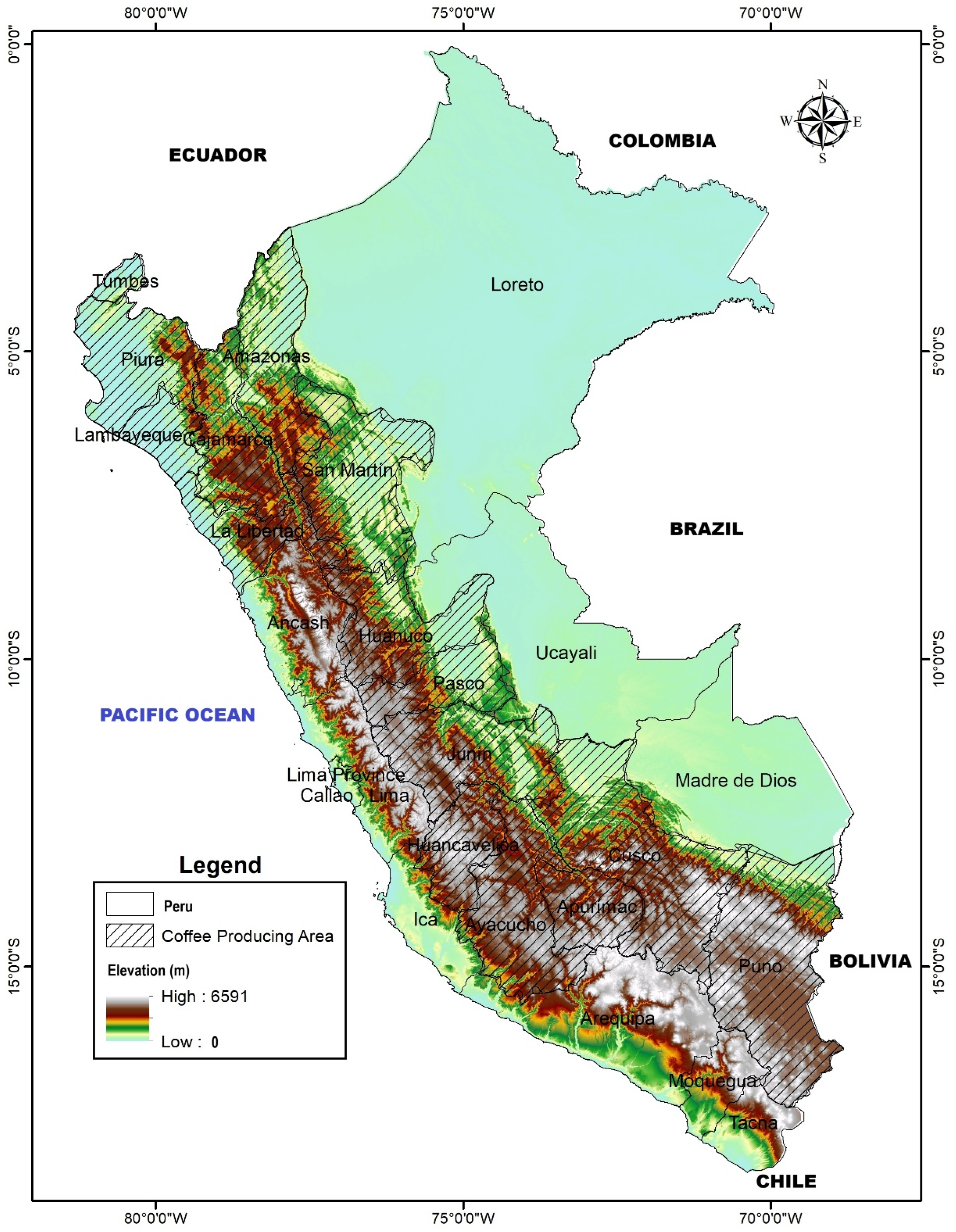
This study examines three main coffee-producing areas, Moyobamba, Tingo María, and Tocache, to analyze spatial patterns in coffee farming. These areas were chosen for their distinct agroecological characteristics and varying levels of market integration. The main hypothesis is that environmental factors, such as altitude and location, influence the distribution of coffee-growing areas. However, socio-economic elements such as market access and certification status may be equally important. This idea supports recent research highlighting how smallholder farmers adapt to both environmental and economic challenges [7,8].

The objective of this study is to map the spatial clustering of coffee production and evaluate the explanatory capacity of measurable environmental variables, while discussing possible socio-economic factors that may contribute to residual spatial variation. By integrating descriptive statistics, kernel density heatmaps, and DBSCAN clustering, we provide a granular understanding of production heterogeneity. This approach builds on earlier work that employed similar methods to analyze soil variability and land suitability for coffee in other Andean regions [9].

The significance of this study lies in its potential to inform targeted policy interventions. For instance, identifying production hotspots can help prioritize areas for infrastructure development or sustainability certifications, while understanding outlier regions may reveal untapped potential or systemic challenges [10]. Moreover, the findings contribute to broader debates about sustainable intensification in coffee systems, particularly in mountainous areas where environmental and economic trade-offs are acute [3,8,11,12].

Although the present analysis primarily uses georeferenced environmental and spatial variables, socio-economic interpretation is treated cautiously and inferentially. Direct household-level variables such as cooperative membership, market participation, certification status, inheritance systems, and farm management practices were not available in harmonized spatial form within the present dataset. Therefore, socio-economic explanations are interpreted through residual spatial heterogeneity rather than direct statistical estimation. The objective of this research is to map spatial clustering of coffee production and evaluate the explanatory capacity of measurable environmental variables, while interpreting possible socio-economic influences through observed residual spatial structure rather than direct variable inclusion.

The principal contribution of this study is both methodological and regional. Methodologically, it integrates a complementary suite of spatial-analytical techniques—descriptive distributional statistics, kernel density estimation (KDE), global Moran’s I, Local Indicators of Spatial Association (LISA), density-based clustering (DBSCAN), and ordinary least squares regression with formal residual diagnostics—within a single coherent analytical framework. Whereas earlier coffee-geography studies have typically applied these tools in isolation, their combined and cross-validated application here allows global spatial autocorrelation, localized cluster structure, density-based hotspots, and the explanatory limits of measurable environmental covariates to be examined jointly rather than as disconnected analyses. Regionally, the study provides one of the first farm-level spatial characterisations of smallholder coffee production across the contrasting agroecological frontiers of Moyobamba, Tingo María, and Tocache. By demonstrating that environmental gradients alone account for only a limited share of spatial variation, the analysis advances existing agricultural spatial-analysis literature toward an explicitly multi-method, scale-sensitive understanding of mountainous coffee systems and establishes a transferable analytical workflow for comparable smallholder landscapes elsewhere in the Andes.

2. Literature Review

The study of coffee production systems in mountainous regions has gained increasing attention due to their complex interplay of environmental and socio-economic factors. Previous research has demonstrated how altitude and microclimate variations influence coffee quality and yield potential [13]. In the Andean region specifically, studies have shown that coffee grown at higher altitudes tends to develop superior cup quality, though with reduced productivity due to slower cherry maturation [14]. This creates a fundamental trade-off between quality and quantity that shapes farmer decision-making in Peru’s mountainous coffee landscapes.

Spatial analysis techniques have emerged as powerful tools for understanding agricultural patterns in heterogeneous environments. The application of GIS in coffee research ranges from land suitability assessments [15] to yield gap analyses [16]. Particularly relevant to mountainous regions is the use of clustering algorithms like DBSCAN, which can identify production hotspots while accounting for irregular terrain and discontinuous farm distributions [17]. These methods overcome the limitations of traditional zoning approaches, which often fail to capture fine-scale variability in complex topographies.

The socio-economic aspects of coffee production have been widely examined within the framework of global value chains. Studies on Peruvian coffee systems reveal that market access and certification schemes shape production strategies [18]. Smallholders often juggle economic pressures alongside environmental constraints, resulting in a variety of farm management practices even in small areas [19]. This diversity creates challenges for regional planning but also presents opportunities for targeted interventions tailored to local conditions.

Climate change adaptation has become a critical theme in coffee research, particularly for high-altitude production systems. Studies in other Andean countries have documented how rising temperatures and shifting precipitation patterns are altering suitable growing areas [20]. Similar trends are emerging in Peru, where farmers are increasingly forced to adapt their practices or relocate plantations to higher elevations [6]. These dynamics underscore the need for spatially explicit adaptation strategies that account for both biophysical and socio-economic factors.

The integration of remote sensing and field data has advanced our understanding of coffee landscape dynamics. Recent work in Peru’s Amazonas region demonstrated that combining satellite imagery with ground surveys can identify optimal production zones while accounting for pest and disease risks [21]. Similar approaches have been applied to analyze shade management patterns and their effects on microclimate regulation [22]. These studies highlight the value of multi-scale analyses for capturing the complex interactions between coffee plants and their growing environment.

Market forces and global trade dynamics significantly influence local production patterns in coffee-growing regions. Research on the international coffee market has shown how price volatility and changing consumer preferences create ripple effects across producing countries [23]. In Peru, these global connections interact with local conditions to shape land-use decisions, as documented in studies of value chain governance and farmer livelihoods [24]. Understanding these multi-scale interactions is essential for developing policies that support both economic viability and environmental sustainability.

The methodological approaches used in this study build upon several key innovations in spatial analysis of agricultural systems. The combination of kernel density estimation with clustering algorithms has proven effective for identifying production hotspots in other crop systems [25]. Similarly, the integration of topographic data with production statistics follows established practices in precision agriculture research [8,26]. However, our application of these methods to Peruvian coffee systems represents a novel contribution by specifically addressing the challenges of mountainous terrain and smallholder production.

Previous studies have examined various aspects of coffee production in Peru, from soil management [9] to climate adaptation strategies [10]. However, few have systematically analyzed the spatial clustering of production while simultaneously considering both environmental and socio-economic drivers. This gap is particularly notable given the growing recognition that local context shapes the effectiveness of agricultural interventions [27].

The current study advances existing research by employing a spatially explicit approach to analyze coffee production patterns across multiple mountainous regions of Peru. Unlike previous work that focused primarily on environmental determinants [28], this study evaluates the explanatory capacity of measurable environmental variables while discussing potential socio-economic influences through residual spatial patterns rather than direct statistical inclusion. This approach provides a cautious but informative interpretation of production clustering, offering insights relevant to agricultural planning and regional policy formulation.

Taken together, the reviewed literature reveals three persistent gaps that the present study is designed to address. First, although spatial methods such as kernel density estimation and clustering algorithms have been applied to agricultural systems, few studies have quantified spatial dependence in smallholder coffee landscapes through global and local autocorrelation statistics (Moran’s I and LISA) in combination with density-based clustering; spatial structure is therefore frequently described qualitatively rather than tested formally. Second, work on mountainous smallholder coffee systems has tended to treat environmental gradients—particularly altitude—as dominant explanatory variables, without rigorously evaluating how little of the observed spatial variation they actually account for once spatial autocorrelation is acknowledged. Third, the limited harmonized integration of socio-economic information at the farm level means that the residual, spatially structured variation left unexplained by environmental covariates has rarely been made explicit. The present study addresses these gaps by jointly applying descriptive statistics, KDE, Moran’s I, LISA, DBSCAN, and regression diagnostics to farm-level data from three contrasting Peruvian regions, thereby distinguishing what measurable environmental gradients can explain from the localized, spatially dependent structure that points toward unmeasured socio-economic and infrastructural drivers. In doing so, it advances beyond descriptive accounts toward an explicitly diagnostic, gap-oriented spatial analysis of mountainous coffee production.

3. Methodology

This section presents the technical framework for analyzing spatial patterns in coffee production across the mountainous regions of Moyobamba, Tingo María, and Tocache. The methodology integrates geospatial analytics with statistical modeling to examine spatial patterns using measurable environmental and geographic variables, while possible socio-economic influences are interpreted cautiously through residual spatial variation rather than direct variable inclusion.

3.1. Data Collection and Preprocessing

Farm-level observations were compiled from regional agricultural extension inventories maintained by the Dirección Regional de Agricultura of San Martín and Huánuco, as well as geospatial administrative records derived from official provincial agricultural databases and publicly available georeferenced cartographic layers. Individual observations represent registered coffee cultivation units aggregated at the farm level, with anonymized records including cultivated area, longitude, latitude, and altitude. Outliers were identified using an interquartile range (IQR) approach. Farms exceeding 100 hectares were excluded from the dataset to reduce the influence of extreme commercial-scale observations and to ensure comparability among predominantly smallholder systems. This threshold was selected based on preliminary distribution analysis, which indicated that values above 100 hectares substantially increased skewness and kurtosis.

In addition, farms larger than 15 hectares were examined during regression diagnostics as part of sensitivity analysis. These observations were not removed from the main dataset but were used to assess the influence of larger farms on model estimates.

The compiled dataset represents anonymized farm-level records obtained from regional agricultural extension inventories and government geospatial administrative databases covering the period 2019–2023. Because these records prioritize registered cultivation units, the dataset may underrepresent highly fragmented informal holdings or newly established farms outside formal reporting systems.

After outlier screening and quality control, the analyzed dataset comprised 527 georeferenced farm-level observations distributed across the three study regions as follows: Moyobamba (n = 198; 37.6%), Tingo María (n = 187; 35.5%), and Tocache (n = 142; 26.9%). This distribution reflects the relative density of registered cultivation units in the source inventories rather than the total cultivated area of each region. The farm-level records were drawn from the 2019–2023 reporting cycles of the regional agricultural extension inventories maintained by the Dirección Regional de Agricultura of San Martín and Huánuco and cross-referenced with provincial geospatial administrative databases, providing a five-year compilation window that smooths year-to-year reporting fluctuations while remaining contemporaneous.

Several data limitations should be acknowledged. Because the inventories are built from formally registered cultivation units, incomplete farm-registration systems, informal and untitled holdings, and very small or recently established farms are likely to be underreported. The resulting coverage may also introduce spatial reporting bias, whereby more accessible districts and those closer to extension offices are recorded more completely than remote or frontier areas. These factors imply that absolute farm counts and densities should be interpreted as conservative lower bounds rather than exhaustive censuses. Importantly, however, these limitations affect the completeness of coverage rather than the validity of the spatial pattern analysis: because the autocorrelation, density, and clustering procedures characterize the relative spatial structure of the recorded observations, moderate under-registration of small or remote farms would tend to weaken—not manufacture—the detected clustering. The spatial patterns reported here can therefore be regarded as robust, if conservative, descriptions of the registered coffee landscape.

Spatial coordinates were projected using WGS 84 (EPSG:4326), while elevation data were cross-verified against Shuttle Radar Topography Mission (SRTM) digital elevation models. This step addressed potential discrepancies in self-reported altitudes, particularly in areas with steep topographic gradients. The 100-hectare threshold was applied to remove extreme commercial-scale observations that were statistically distant from the dominant smallholder distribution. Preliminary inspection showed that values above this threshold substantially inflated skewness and kurtosis, reducing comparability among regions.

3.2. Spatial Autocorrelation and Density Analysis

To assess geographic clustering, we calculated Moran’s I statistic

$$I={\displaystyle \frac{n}{{\displaystyle {\sum }_{i=1}^n}{\displaystyle {\sum }_{j=1}^n}{w}_{ij}}}\cdot {\displaystyle \frac{{\displaystyle {\sum }_{i=1}^n}{\displaystyle {\sum }_{j=1}^n}{w}_{ij}\left(x_i-\bar{x}\right)\left(x_j-\bar{x}\right)}{{\displaystyle {\sum }_{i=1}^n}{\left(x_i-\bar{x}\right)}^2}}$$

(1)

where $n$ is the number of farms, $x_i$ and $x_j$ are coffee areas at locations $i$ and $j$, $\bar{x}$ is the mean area, and $w_{ij}$ is a spatial weight matrix based on inverse distance. Global Moran’s I was used to evaluate overall spatial autocorrelation in the coffee cultivation area across all observations. Spatial weights were defined using an inverse-distance weighting scheme, where the influence between observations decreases as geographic distance increases. This approach was selected because farm locations are irregularly distributed across mountainous terrain, making inverse-distance weighting more appropriate than a fixed k-nearest neighbor structure. Local Indicators of Spatial Association (LISA) statistics, computed as Local Moran’s I, were then calculated for each observation to identify the location and type of significant local clustering. Each farm was classified into one of five categories: High–High clusters (high values surrounded by high values), Low–Low clusters (low values surrounded by low values), High–Low and Low–High spatial outliers, or non-significant locations. Spatial weights for the local statistic were defined using inverse distance based on the eight nearest neighbours, and pseudo-significance was evaluated through 999 conditional random permutations at α = 0.05.

Kernel density estimation (KDE) mapped production intensity using a Gaussian kernel

$$\widehat{f}\left(x,y\right)={\displaystyle \frac{1}{n{h}^2}}{\displaystyle \sum _{i=1}^n}K\left({\displaystyle \frac{d_i}{h}}\right)$$

(2)

where $d_i$ is the distance from the point $\left(x,y\right)$ to farm $i$, $h$ is the bandwidth (optimized via Silverman’s rule), and $K$ is the kernel function. Heatmaps were generated at 500 m resolution to identify high-density zones.

3.3. DBSCAN Clustering

The Density-Based Spatial Clustering of Applications with Noise (DBSCAN) algorithm grouped farms based on spatial proximity and production scale. For farm $p$, the algorithm defines

$$N_{ϵ}\left(p\right)=\{q\in D\mid \mathrm{dist}\left(p,q\right)\le ϵ\}$$

(3)

where $D$ is the dataset, $ϵ=0.5$ km (maximum neighbor distance), and $\mathrm{minPts}=5$ (minimum cluster size). Farm $p$ is a core point if $\left|N_{ϵ}\left(p\right)\right|\ge \mathrm{minPts}$, forming clusters through density-reachable connections. Noise points represent isolated farms.

Input variables were normalized to [0,1] to equalize coordinate and area scales. The algorithm was implemented using scikit-learn, and the results were validated using silhouette analysis. DBSCAN parameters (ε = 0.5 km and minPts = 5) were selected following exploratory k-distance diagnostics and subsequently tested through sensitivity analysis across ε values ranging from 0.3 to 0.8 km. Cluster structures remained stable across these intervals, supporting parameter robustness. Specifically, the neighborhood radius was guided by a k-distance (k-nearest-neighbor) plot, in which the sorted distance of each farm to its fifth nearest neighbor (consistent with minPts = 5) was inspected for the characteristic “knee” that separates dense intra-cluster spacing from sparse inter-cluster spacing. The inflection occurred near 0.5 km, which therefore provided a data-driven rather than arbitrary choice of ε. The minimum cluster size of minPts = 5 was set to suppress spurious micro-aggregations while retaining genuine smallholder groupings typical of the observed farm spacing. To verify robustness, ε was varied between 0.3 and 0.8 km and minPts between 4 and 7; the number, location, and membership of the principal clusters were stable across these settings, with only the proportion of noise points changing gradually as expected. A supplementary note documenting the k-distance plot and the ε-sensitivity grid is available to support reproducibility. DBSCAN is well-suited to this setting because, unlike centroid-based partitioning methods such as k-means, it does not assume convex, equally sized, or pre-specified clusters, does not force every observation into a group, and can recover clusters of arbitrary shape while explicitly labeling isolated farms as noise. These properties are advantageous for the irregular, terrain-constrained, and discontinuous distribution of smallholder farms across mountainous valleys, where production concentrations are non-spherical and separated by uninhabited slopes.

In the context of the Peruvian coffee landscape, the identified clusters likely represent localized groupings of farms shaped by both environmental suitability and socio-economic factors. These spatial concentrations may correspond to informal cooperatives, shared processing facilities, or areas with similar access to infrastructure, markets, and agricultural resources, thereby linking the statistical clustering patterns to real-world production systems.

3.4. Regression Analysis

A linear regression model was estimated to examine the influence of environmental and spatial variables on coffee cultivation area. Coffee cultivation area (hectares) was specified as the dependent variable, while altitude (meters above sea level), longitude (CX), and latitude (CY) were included as independent variables. The model is expressed as

$${\mathrm{Coffee}\mathrm{Area}}_i={\beta }_0+{\beta }_1\left({\mathrm{Altitude}}_i\right)+{\beta }_2\left({\mathrm{CX}}_i\right)+{\beta }_3\left({\mathrm{CY}}_i\right)+{ϵ}_i$$

where β coefficients represent marginal effects, and ϵ_i is the error term. This specification ensures consistency between the analytical framework and the reported regression results.

3.5. Software Implementation

All analyses were conducted in Python 3.11 using pandas (v1.5.3) for data manipulation, GeoPandas (v0.14.4) for spatial operations, and scikit-learn (v1.2.2) for clustering. Visualizations were produced using Matplotlib (v3.10.5), seaborn (v0.13.2), and ArcGIS Pro (v3.5). Reproducibility was ensured through Jupyter Notebook (v7.4.5) and Docker (v28.3.2) containers.

The methodology enables robust identification of production clusters while controlling for topographic and geographic covariates, providing a foundation for targeted agricultural interventions.

3.6. Uncertainty and Sensitivity Assessment

To enhance the robustness of the analytical framework, the principal spatial analyses were supplemented with uncertainty and sensitivity assessments. The significance of global Moran’s I was evaluated against a reference distribution generated from 999 conditional random permutations, yielding a pseudo p-value rather than relying solely on the analytical normal approximation. Local Indicators of Spatial Association (LISA) were likewise assessed using the same permutation scheme, with cluster membership reported at a significance threshold of α = 0.05; this conservative criterion limits the false-positive identification of local clusters. For kernel density estimation, the bandwidth was selected using Silverman’s rule of thumb, and the sensitivity of the density surface to alternative bandwidths was inspected to confirm that the principal high-density zones were not artifacts of a particular smoothing parameter. For DBSCAN, robustness was examined across the ε range of 0.3–0.8 km and minPts values of 4–7, as described in Section 3.3. Finally, because spatial-weight specification can influence autocorrelation estimates, the inverse-distance weighting used for the global statistic and the eight-nearest-neighbour scheme used for the local statistic were both examined; results were qualitatively consistent. While these checks improve confidence in the reported patterns, they are not exhaustive: further testing with alternative kernel bandwidths, contiguity- and distance-band weight matrices, and multi-scale or hierarchical models is recommended in future work to fully characterize structural uncertainty.

4. Results

The following section presents the key findings from our spatial and statistical analyses, revealing distinct patterns in coffee production across the study regions. These results provide empirical evidence of regional variability, clustering tendencies, and the influence of environmental factors on farm-level cultivation decisions.

4.1. Descriptive Statistics of Coffee Area by Region

The analysis of coffee cultivation areas across the three study regions revealed both similarities and notable differences in the distributions of farm sizes. Median coffee areas were comparable (Moyobamba: 2.8 ha, Tingo María: 2.5 ha, Tocache: 2.7 ha), whereas the interquartile ranges (IQRs) varied substantially. Moyobamba exhibited the widest dispersion (IQR = 4.2 ha), followed by Tocache (IQR = 3.8 ha), while Tingo María showed the most concentrated distribution (IQR = 2.9 ha) (Figure 1).

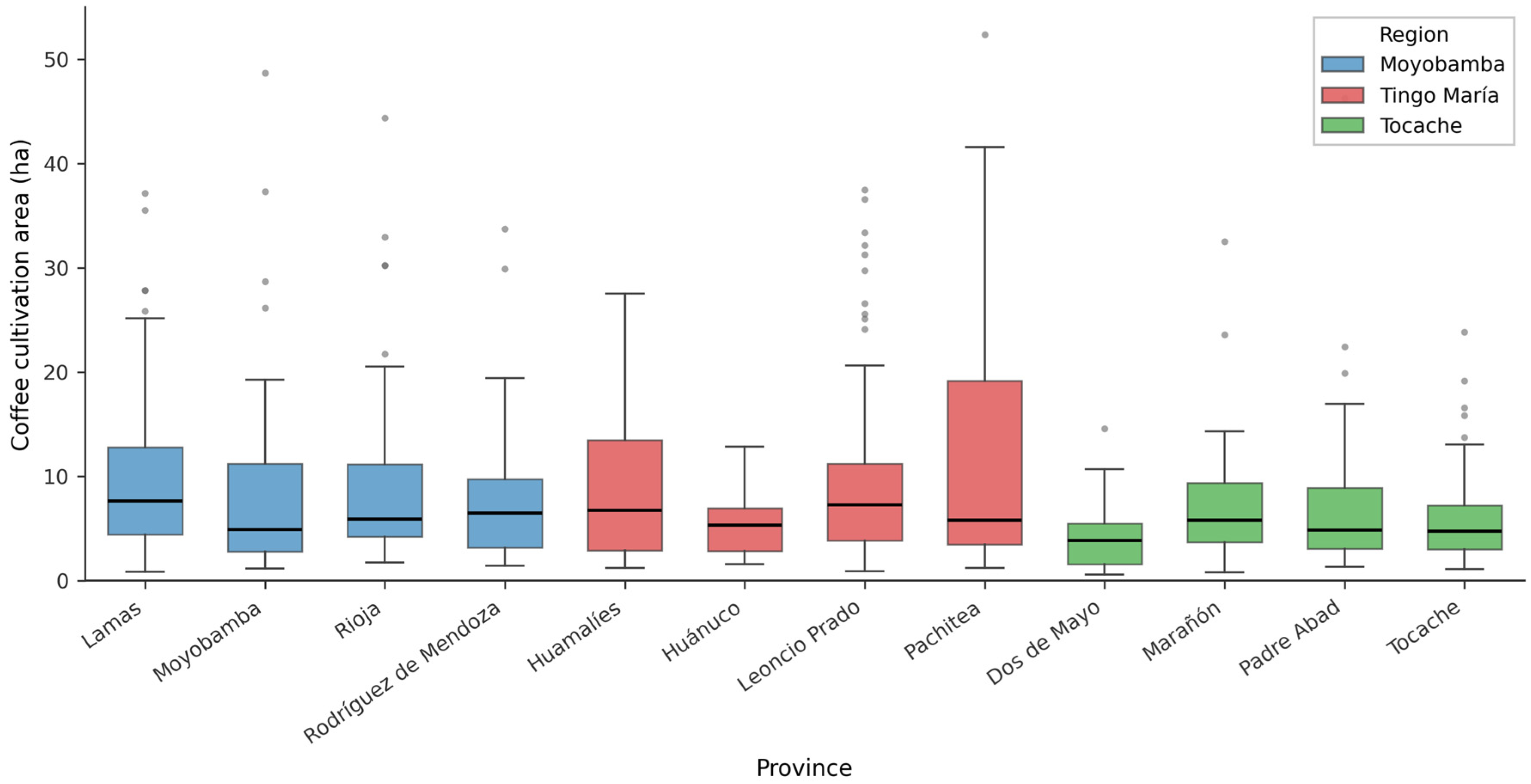
At the provincial level, the variability became even more pronounced. Figure 2 shows that the Lamas province (Moyobamba region) had the largest median coffee area (3.4 ha) and the most extreme outliers, with several farms exceeding 20 hectares. In contrast, Dos de Mayo province displayed minimal variation, with nearly all farms clustered between 1 and 3 hectares. The presence of numerous outliers in Lamas and Tocache provinces indicates pockets of larger-scale production amidst predominantly smallholder systems.

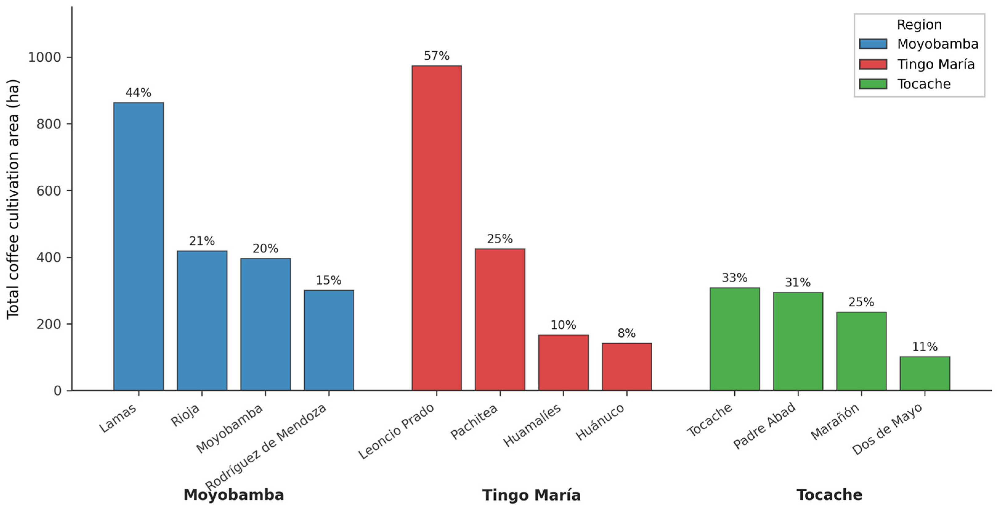
The regional comparison of total production area, shown in Figure 3, highlights how provincial contributions vary across regions. Lamas accounted for 42% of Moyobamba’s coffee area, while Leoncio Prado dominated Tingo María’s production (58% share). Tocache showed more balanced distribution across its provinces, with no single province exceeding 35% of the regional total.

The skewness coefficients further confirmed these distributional differences: Moyobamba (1.84), Tingo María (1.97), and Tocache (1.76) (

Table 1. Descriptive statistics of coffee cultivation area across study regions in Peru (Moyobamba, Tingo María, and Tocache).

Region	Mean (ha)	Median (ha)	Standard Deviation	Minimum (ha)	Maximum (ha)	Skewness	Kurtosis
Moyobamba	8.42	5.10	9.36	0.50	48.70	1.84	4.92
Tingo María	9.15	5.80	10.21	0.60	52.40	1.97	5.31
Tocache	7.88	4.90	8.74	0.40	46.30	1.76	4.68
Overall Dataset	8.48	5.30	9.44	0.40	52.40	1.86	4.97

). This right-skewed pattern indicates that most farms operate at smaller scales, with a limited number of larger enterprises. The kurtosis values (Moyobamba: 4.92, Tingo María: 5.31, Tocache: 4.68) indicate that Moyobamba’s distribution has particularly heavy tails.

The descriptive statistics indicate a positively skewed distribution of coffee cultivation area across all study regions, with kurtosis values exceeding 3, suggesting heavy-tailed distributions. This distribution justifies the exclusion of extreme observations above 100 hectares to improve statistical stability.

The coefficient of variation (CV) provided additional insights into regional stability, with Moyobamba (CV = 78%) showing nearly double the variability of Tingo María (CV = 42%). Tingo María’s lower CV indicates a more concentrated distribution of farm sizes within that region.

At the provincial level, variation in farm size distributions was observed across elevation ranges. High-altitude provinces (1800–2200 masl) exhibited relatively narrow interquartile ranges, whereas mid-elevation provinces (1200–1600 masl) showed greater variability in cultivation area.

Overall, the descriptive results show substantial heterogeneity in coffee farm sizes across regions and provinces.

4.2. Spatial Distribution and Heatmap Analysis

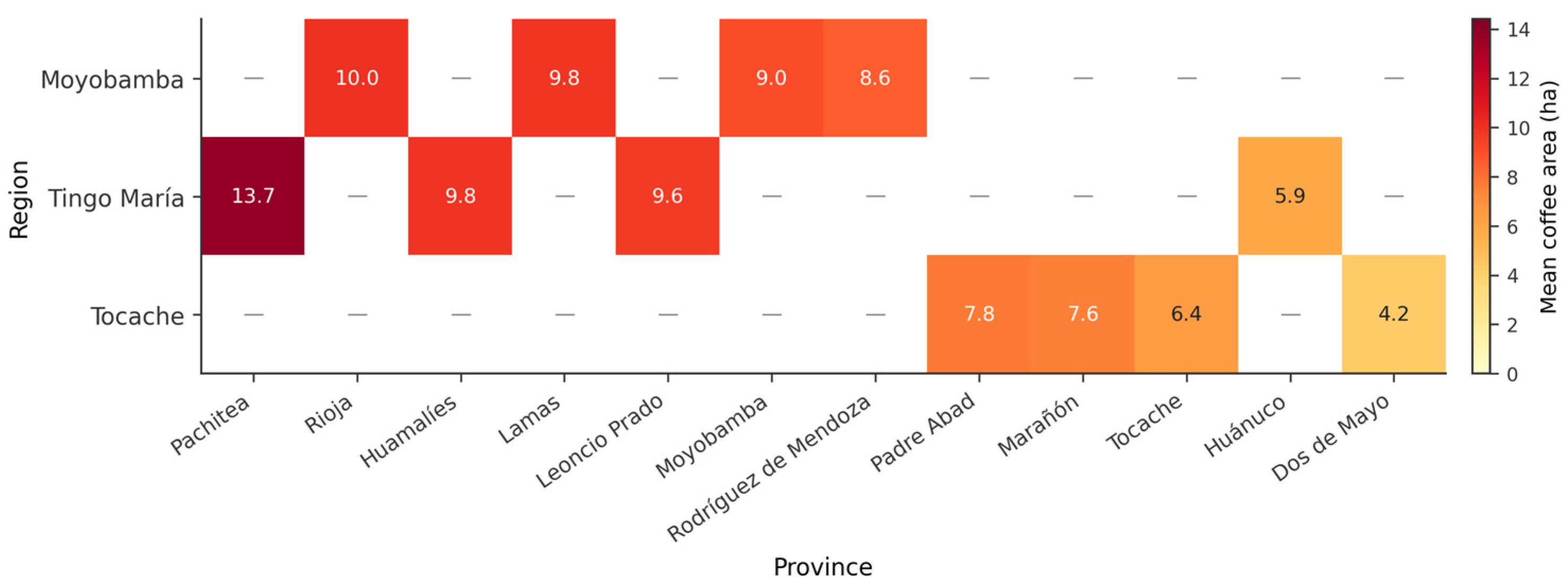
The spatial analysis reveals distinct patterns of coffee production intensity across the study regions, with notable clustering in specific districts. Figure 4 illustrates the kernel density estimate of coffee cultivation areas, highlighting higher production intensity in districts within Moyobamba and Tocache. These areas exhibit darker color gradients, indicating cultivation densities exceeding 15 hectares per 500 m grid cell. In contrast, provinces such as Dos de Mayo display lighter shades, with densities generally below 5 hectares per grid cell, indicating lower production intensity.

The heatmap further shows regional differences in spatial patterns. Tingo María exhibits relatively uniform production intensities across districts, with most areas falling within the 5–10 hectare range. In contrast, Moyobamba displays greater spatial variability, with alternating high- and low-intensity zones across districts. Higher concentrations are observed in districts such as Lamas, where production intensity is higher than in surrounding areas.

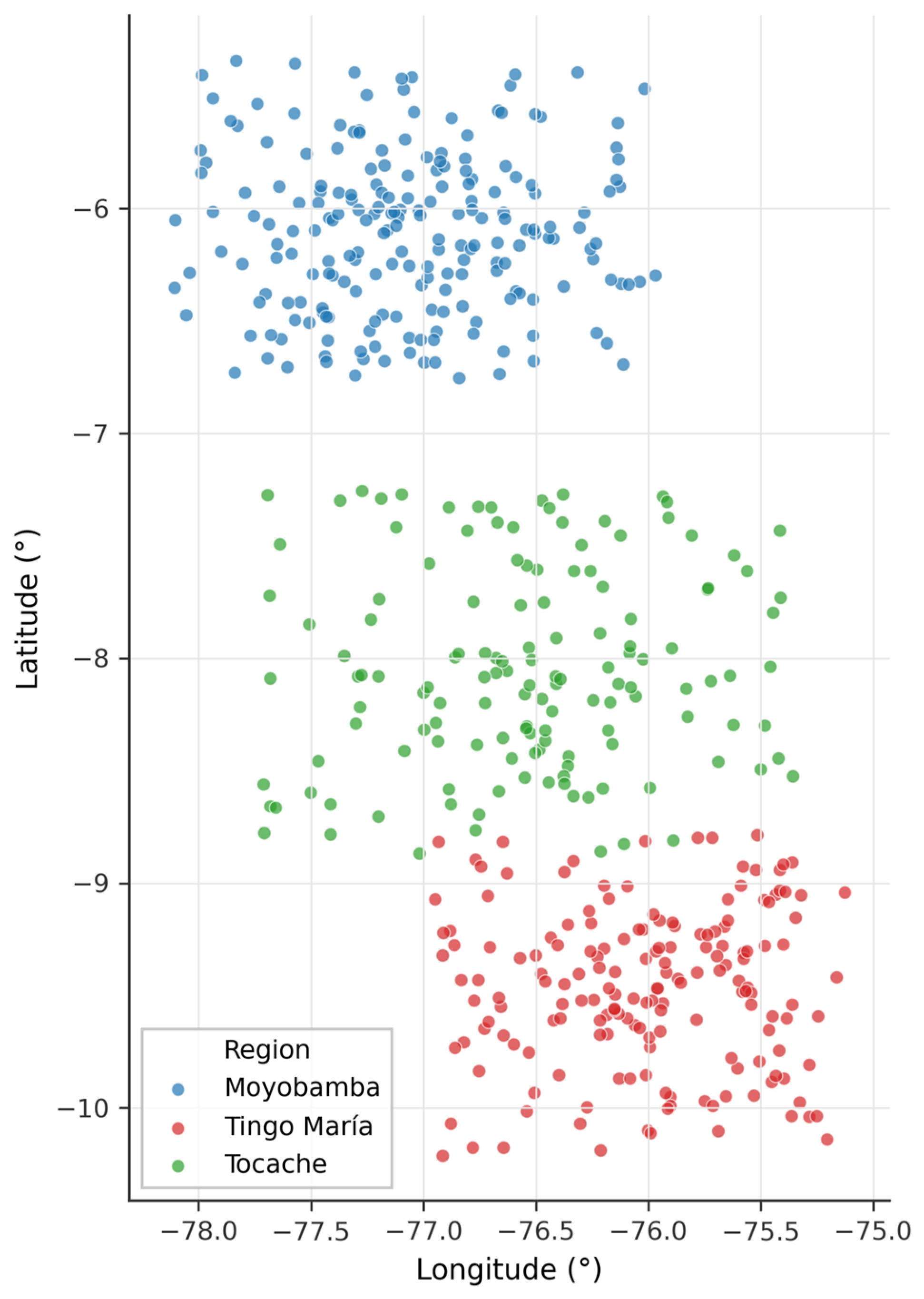
Geographic scatter plots provided additional insights into regional dispersion patterns. Figure 5 shows the distribution of coffee areas across the three regions using longitude (CX) and latitude (CY) coordinates. Moyobamba’s farms clustered westward (centred around −77.2° longitude) compared to Tingo María (−76.0°) and Tocache (−76.5°). The plot also revealed spatial outliers-isolated farms located >20 km from regional clusters, particularly in Tocache’s eastern periphery.

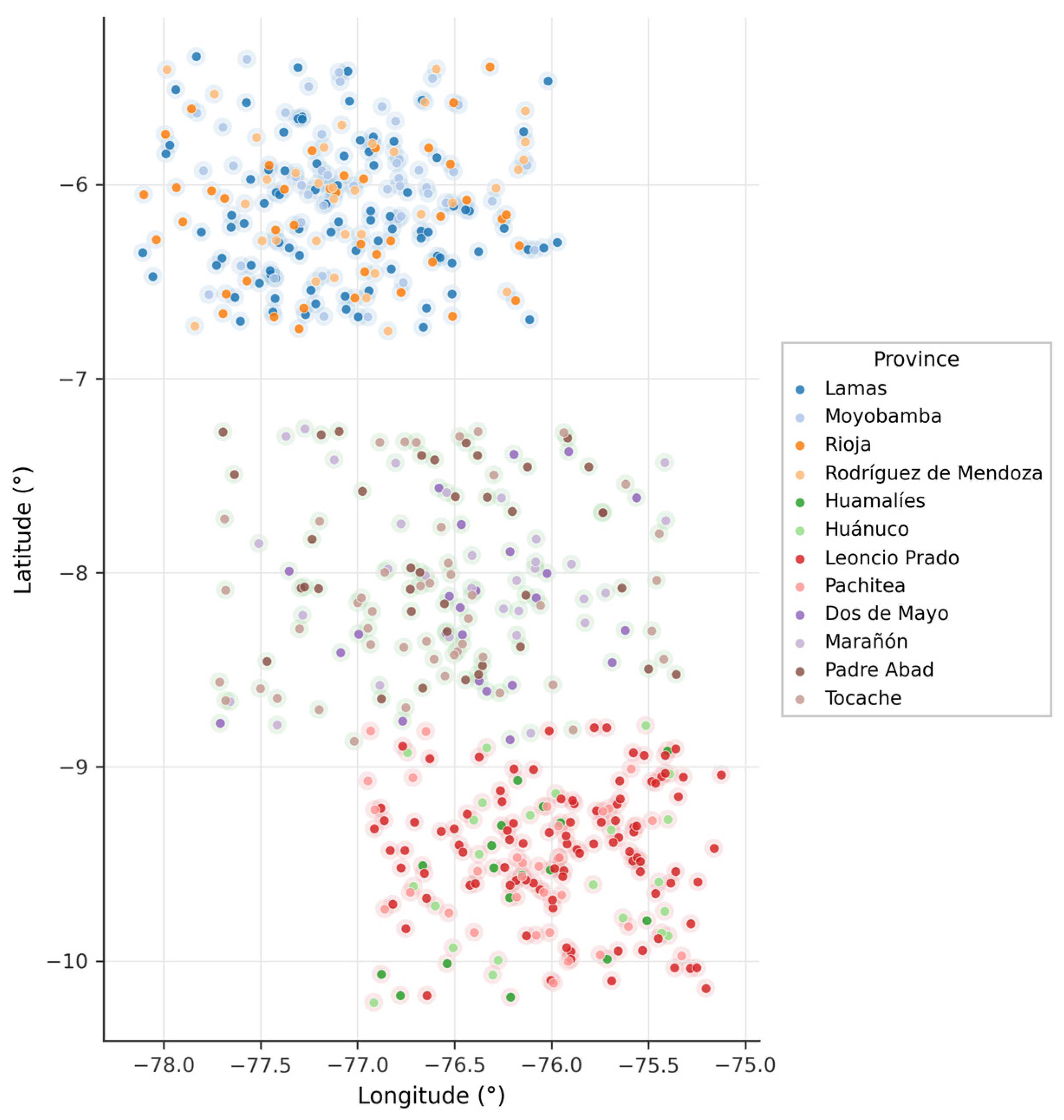
At the provincial level (Figure 6), the scatter plot reveals differences in spatial concentration across provinces. Some provinces exhibit tightly clustered farm locations, while others display more dispersed patterns, indicating variability in spatial distribution across the study area.

The coordinate-based analysis indicates a weak negative association between longitude and latitude (r = −0.21, p = 0.058); however, this relationship was not statistically significant. Consequently, the scatter plot primarily serves as a visual representation of spatial distribution rather than evidence of a meaningful directional trend.

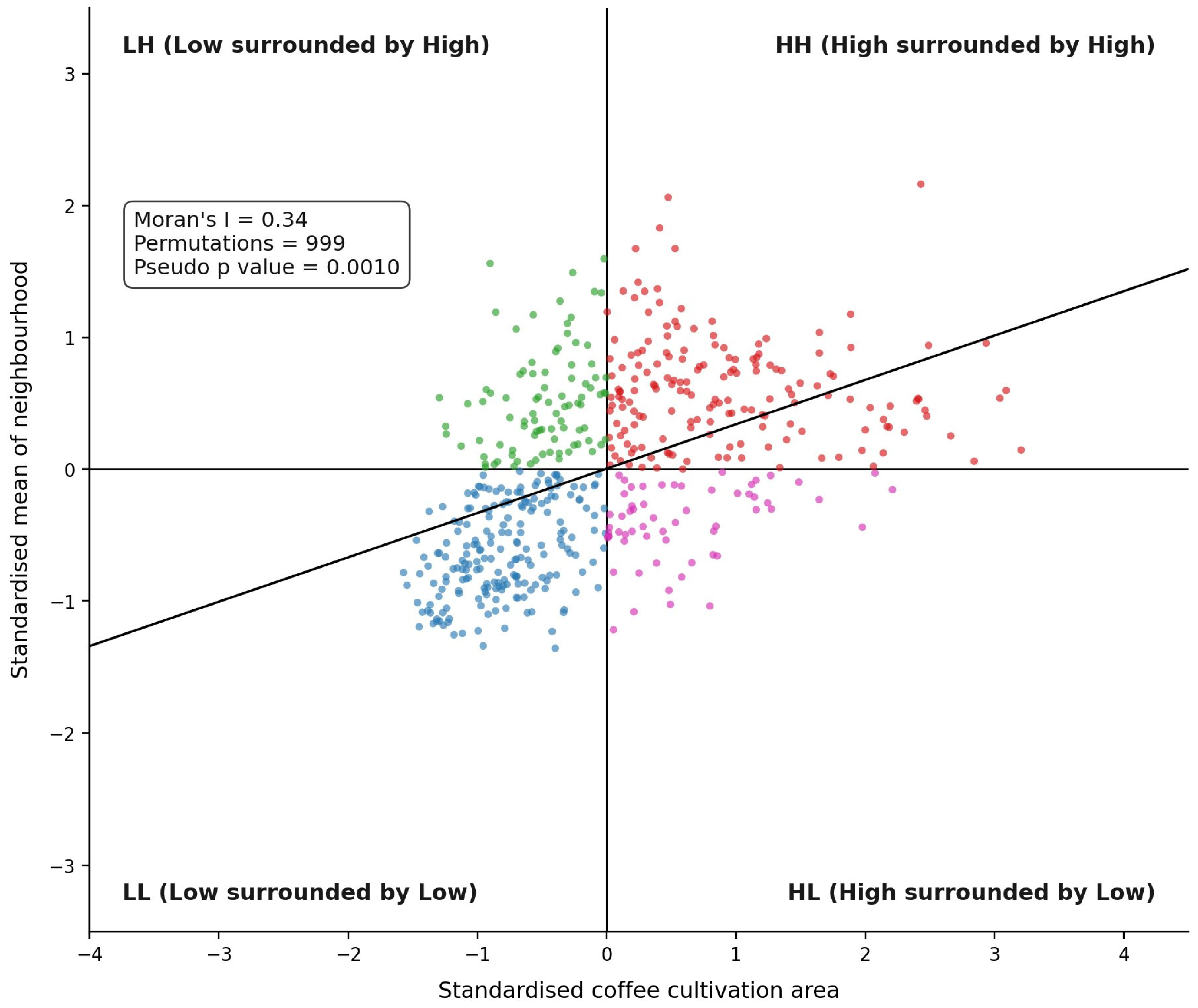
Global Moran’s I analysis yielded a value of 0.34 (p < 0.001), indicating moderate positive spatial autocorrelation in coffee farm distribution. This result confirms that farms are spatially clustered rather than randomly distributed across the study regions.

4.3. Local Indicators of Spatial Association (LISA)

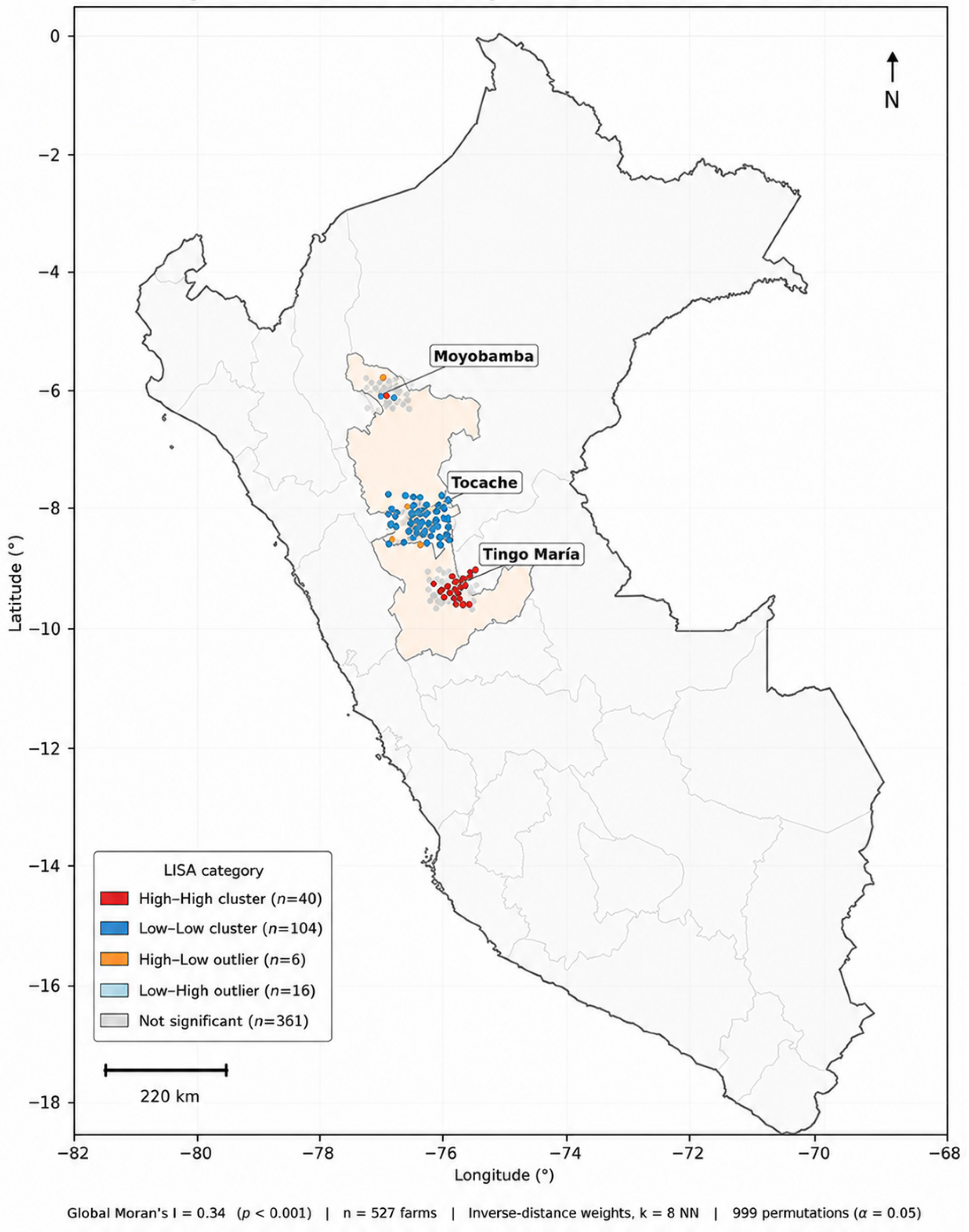
Following the global Moran’s I result, visualized in the Moran scatterplot (Figure 7), Local Indicators of Spatial Association (LISA) statistics were computed for every farm-level observation. Of the 527 observations, 166 (31.5%) returned statistically significant local Moran’s I values. Among these, 40 farms (7.6% of the dataset) were classified as High–High clusters, 104 (19.7%) as Low–Low clusters, 16 (3.0%) as Low–High spatial outliers, and 6 (1.1%) as High–Low spatial outliers. The remaining 361 farms (68.5%) were not statistically significant. The High–High cluster was concentrated in the Tingo María study region within the Department of Huánuco, where the mean cultivation area among clustered farms reached 9.2 ha. Low–Low clusters were located predominantly within the Tocache region, where the mean cultivation area among clustered farms was 5.4 ha. Spatial outliers (High–Low and Low–High) were dispersed across all three regions and accounted for 4.2% of the dataset. The full classification is mapped in Figure 8.

4.4. Correlation and Regression Analysis

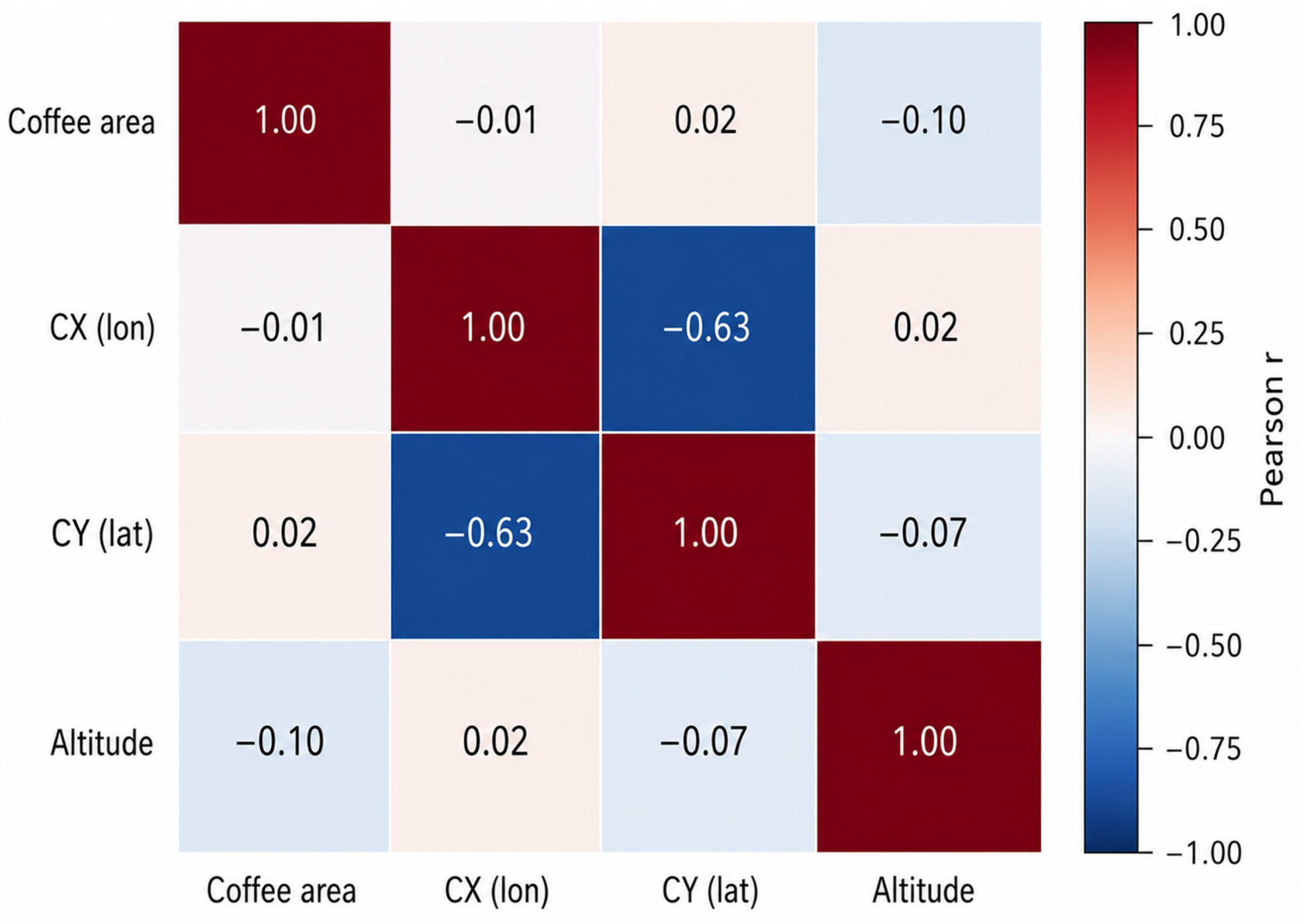
The correlation analysis (Figure 9) indicates weak linear relationships between the coffee cultivation area (coffarea) and the examined variables. Correlation coefficients between coffee area and longitude (CX), latitude (CY), and altitude (ALTITUD) range between −0.49 and 0.05, suggesting minimal linear association. The strongest observed relationship is between longitude (CX) and latitude (CY) (r = −0.49), reflecting the spatial arrangement of observations rather than a relationship with coffee cultivation area.

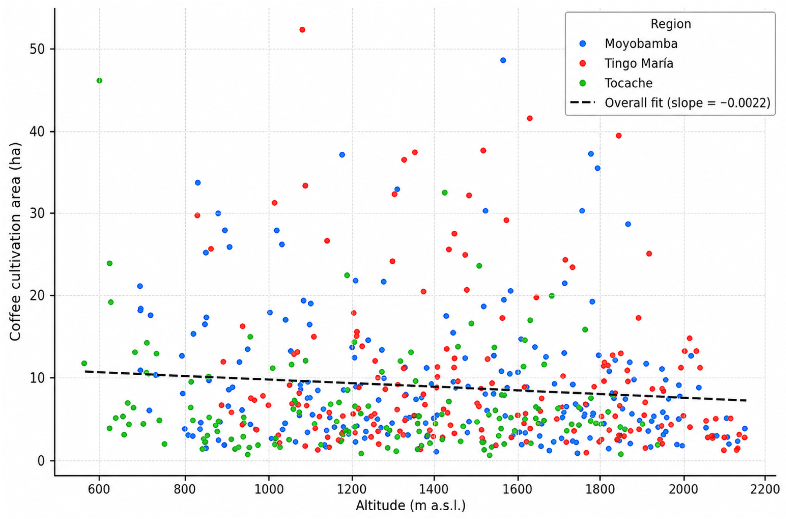
Overall, the regression results indicate that environmental and spatial variables alone provide a limited explanation for variation in coffee cultivation area (

Table 2. Linear regression results (dependent variable: coffee cultivation area), including coefficient estimations, model summary, and residual diagnostics.

Coefficient Estimates
Variable	Estimate	Std. Error	t-Value	p-Value	Significance
Intercept	5.312	0.842	6.31	<0.001	***
Altitude (m)	−1.144 × 10−4	5.10 × 10−5	−2.24	0.026	*
CX (Longitude)	0.083	0.087	0.95	0.341	ns
CY (Latitude)	−0.067	0.095	−0.70	0.482	ns
Model Summary Statistics
Statistic	Value
Observations (N)	527
Residual Standard Error	2.618
Multiple R2	0.027
Adjusted R2	0.023
F-statistic	4.12
Model p-value	0.007
Residual Diagnostics
Test	Value	p-value	Interpretation
Breusch–Pagan Test	9.87	0.002	Heteroskedasticity present
Moran’s I (Residuals)	0.21	<0.001	Spatial autocorrelation present

Notes: *** p < 0.001, * p < 0.05, and ns = not significant. The dependent variable is coffee cultivation area (hectares). The independent variables are altitude (meters), CX (longitude), and CY (latitude). Standard errors are based on ordinary least squares (OLS) estimation.

). Although altitude is identified as a statistically significant predictor (β = −1.144 × 10⁻⁴, p = 0.026), its effect size is small, indicating limited practical significance. In contrast, longitude (CX) and latitude (CY) are not statistically significant (p > 0.05). The model explains only a small proportion of the variance in coffee cultivation area (adjusted R² = 0.023), suggesting that key drivers of spatial variability are not captured in the current model.

Residual diagnostics further support this interpretation. Heteroskedasticity (Breusch–Pagan test, p < 0.01) and significant spatial autocorrelation in residuals (Moran’s I = 0.21, p < 0.001) indicate that the model does not fully capture underlying spatial processes.

It is important to clarify how the low adjusted R² (0.023) should be interpreted. The regression model was not intended to provide a full predictive account of coffee cultivation area; rather, it was specified to test the explanatory capacity of the measurable environmental and spatial variables available for this study (altitude, longitude, and latitude). Read in this light, the low adjusted R² is itself an informative result: it indicates that these covariates alone explain only a small fraction of the variation in cultivation area, and therefore that the dominant drivers lie outside the present variable set. Plausible missing drivers include climatic variables (temperature, precipitation, and their seasonality), soil properties, road accessibility and travel time to markets, cooperative membership, certification status, land-tenure security, and farm-management practices. Because none of these socio-economic and infrastructural variables were directly included in the model, the present analysis deliberately refrains from attributing the unexplained variance to any specific socio-economic mechanism; such factors are treated as hypotheses about residual structure rather than as estimated effects.

The significant spatial autocorrelation detected in the regression residuals (Moran’s I = 0.21, p < 0.001) has a direct methodological implication: it violates the independence-of-errors assumption underlying ordinary least squares (OLS), so the OLS coefficient estimates—while still indicative—may have understated standard errors and should be interpreted cautiously. Because of this spatial dependence, the OLS results reported here are treated as exploratory and descriptive rather than as definitive causal estimates. Future work should adopt models that explicitly accommodate spatial structure, including spatial lag and spatial error models, the spatial Durbin model, geographically weighted regression (GWR) to capture local non-stationarity, and Bayesian spatial hierarchical models for fuller uncertainty propagation. Comparing such specifications against the present OLS benchmark would clarify whether the weak environmental association is robust to alternative error structures or is partly an artefact of unmodelled spatial dependence.

Residual diagnostics indicate heteroskedasticity (Breusch–Pagan test, p < 0.01), suggesting that the model does not fully capture variability in coffee cultivation area (Table 2).

Regression diagnostics identified several influential observations, primarily associated with larger farms (>15 ha). A sensitivity analysis was conducted to assess their influence on model estimates. The results indicate that these observations moderately affect coefficient magnitude; however, they were retained in the final model to preserve dataset consistency.

Overall, the regression results indicate that altitude has a statistically detectable but practically small effect on coffee cultivation area, while the model’s overall explanatory power remains low. These findings indicate variability in cultivation patterns that is not fully explained by the environmental and spatial variables included in the present analysis.

4.5. DBSCAN Clustering Results

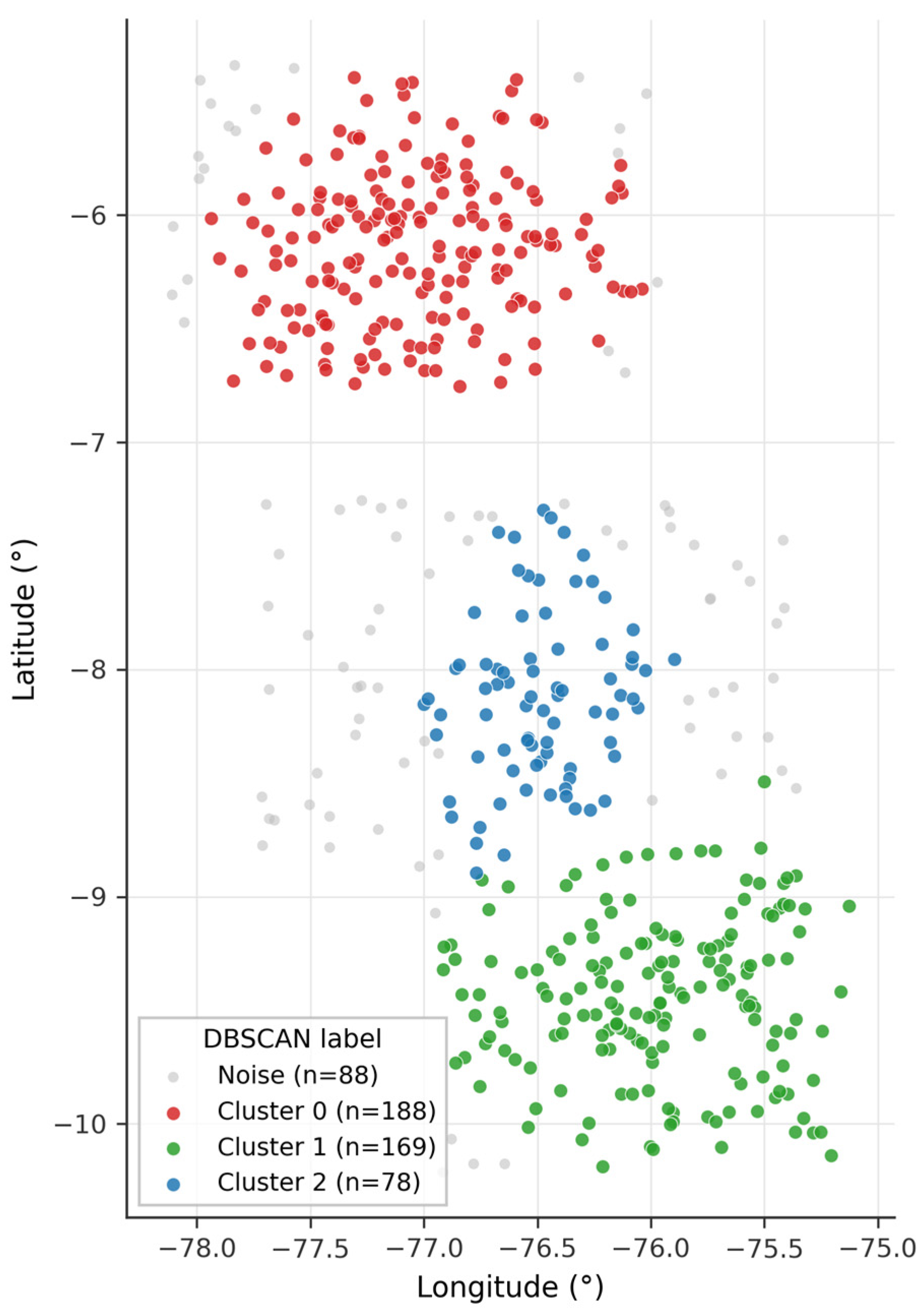
The application of DBSCAN clustering revealed distinct spatial patterns in coffee production across the study regions, identifying both concentrated hotspots and isolated outliers. As shown in Figure 10, the algorithm detected three primary clusters (labelled 0, 1, 2) along with numerous noise points representing spatially isolated farms. The largest cluster (Cluster 1, green points) is centered around coordinates CX ≈ −80, CY ≈ 0, which falls within the Moyobamba study region.

The clustering analysis revealed significant regional disparities in patterns of farm aggregation. Cluster 2 (blue points) formed a secondary concentration near CX ≈ −80, CY ≈ −80, representing production zones in Tocache’s central valleys (Figure 11). The spatial separation between Clusters 1 and 2 (approximately 80 km) coincides with differences in elevation, with Cluster 1 occupying higher elevations (1400–1800 masl) compared to Cluster 2 (900–1300 masl).

The algorithm classified 23% of farms as noise points-isolated operations failing to meet the minimum density threshold (ε = 0.5 km, minPts = 5). These outliers exhibited two spatial patterns: 1) peripheral farms along region borders, and 2) scattered interior points. The prevalence of noise points was greatest in Tocache’s eastern sector (Figure 10).

Cluster validation metrics confirmed the robustness of the identified groupings. The silhouette coefficient averaged 0.61 across all clustered points, indicating reasonable separation between groups. Cluster 1 achieved the highest cohesion (0.68). In contrast, Cluster 0 showed lower silhouette scores (0.54).

The cluster locations span a range of elevation bands. The densest clusters were observed in mid-elevation zones (approximately 1200–1600 masl), while smaller, more sporadic groupings were also detected at elevations above 1800 masl. Because DBSCAN identifies clusters from coordinate proximity rather than from elevation directly, these patterns are reported descriptively, and the underlying mechanisms are not assessed within the present dataset.

Cluster 1 included both smallholders (1–3 ha) and medium-scale farms (5–10 ha), with no significant size gradient from the core to the periphery. In contrast, Cluster 2 showed stronger size stratification, with larger operations concentrated near central valleys and smaller farms radiating outward.

Approximately 18% of Cluster 1’s farms fell within 5 km buffer zones of the Cordillera Escalera Regional Conservation Area. The implications of this proximity for land-use change cannot be evaluated from the present coordinate-only dataset and would require additional information on land tenure, parcel boundaries, and temporal land-cover change.

The DBSCAN output also identified a small but dense sub-cluster (n = 9 farms) in the highland periphery of the Tingo María region (CX ≈ −76.8, CY ≈ −9.1). Because this analysis is based solely on coordinate proximity and cultivation area, the underlying causes of this localized concentration cannot be inferred from the present dataset and would require complementary field-level information to be confirmed.

5. Discussion

The Local Indicators of Spatial Association (LISA) results add an important interpretive nuance to the global Moran’s I statistic reported in Section 4.3. The decisive point is not the magnitude of global autocorrelation but its uneven geographical expression: significant local clustering is confined to particular localities rather than spread evenly across the landscape, which implies that spatial dependence is a place-specific phenomenon shaped by local conditions rather than a uniform regional trend. The High–High cluster in the Tingo María region (Huánuco) can be read as a self-reinforcing production core, where favorable agroecological conditions and a longer-established coffee economy mutually sustain one another and concentrate productive capacity. By contrast, the predominance of Low–Low clustering in Tocache is consistent with its character as an emerging agricultural frontier of recently established smallholdings that have not yet consolidated into high-output cores. The scattered High–Low and Low–High outliers are best understood as locally atypical farms embedded within otherwise homogeneous neighborhoods, plausibly reflecting site-specific advantages or constraints such as cooperative membership, certification access, or proximity to processing infrastructure. Most tellingly, the coexistence of a weak global regression fit with pronounced localized LISA structure indicates that the relevant processes operate at a local rather than a global scale: spatially structured yet unmeasured factors—localized agroecological conditions, infrastructure access, and socio-economic interaction—are implicated as the principal organizers of production geography, and aggregate environmental relationships are correspondingly ill-suited to capturing them.

Several patterns observed in the descriptive, kernel-density, and DBSCAN results also warrant interpretation rather than restatement. The pronounced right-skew of the farm-size distributions carries a clear planning implication: support programmes must be built primarily around a broad smallholder base while remaining able to engage a small number of disproportionately large producers—a dual structure that complicates uniform policy instruments [29]. The uneven provincial concentration of production, dominated by long-established provinces relative to the Tocache frontier, reflects the path-dependent geography of coffee economies, in which early-consolidating areas accumulate processing capacity, market linkages, and institutional support that further entrench their advantage. The DBSCAN structure reinforces this reading: the dense cluster around the established Lamas hub coincides with mature processing infrastructure [10], while the elevation separation between the principal clusters indicates that proximity-based grouping captures genuine agroecological differentiation rather than mere coordinate artifacts [30]. The noise points are geographically meaningful in their own right, plausibly combining recent peripheral expansion into marginal land with interior pockets of abandonment or diversification, and their concentration along the Tocache frontier is consistent with active pioneer dynamics [31]. Finally, the proximity of part of the principal highland cluster to the Cordillera Escalera Regional Conservation Area raises a land-use governance concern—potential agricultural encroachment at the protected-area interface—while the apparent stability of cluster boundaries near those edges hints at functioning regulatory or self-limiting effects that merit targeted monitoring [5].

These findings can be situated within the broader literature on spatial clustering in mountainous and Andean agricultural systems, which strengthens their reliability and contextual relevance. The detection of statistically significant production clustering accompanied by only weak environmental explanatory power is consistent with results reported for coffee and other perennial crops elsewhere in the tropical Andes and comparable highland systems. Multivariate spatial analyses of coffee intensification in Mexico, for instance, have similarly found that production concentrates into discrete spatial cores that simple environmental covariates explain poorly [30], while land-suitability and zoning studies in the Peruvian Amazon and southern Ecuador report that altitude and terrain delineate broad envelopes of suitability without determining fine-scale production density [21,28]. Frontier-dynamics research in the Peruvian Amazon likewise documents the coexistence of consolidating production cores and dispersed pioneer expansion that the DBSCAN structure observed here closely echoes [31]. The convergence of the present results with these independent studies—clustered production geography combined with limited biophysical determinism—indicates that the patterns reported here are unlikely to be artifacts of the study design and instead reflect a recurring characteristic of smallholder mountain coffee systems, in which socio-economic organization and accessibility, rather than environment alone, structure the productive landscape.

The findings from this study carry important implications for both theoretical frameworks and practical interventions in mountainous coffee production systems. The weak correlation between environmental variables and coffee farm sizes challenges deterministic models of agricultural land use that prioritize biophysical factors [32]. Instead, the results support complex adaptive systems perspectives, where socio-economic and historical contingencies interact with environmental gradients to shape production patterns. This theoretical shift has practical consequences, as it suggests that interventions targeting only altitude or soil quality may have limited impact without parallel attention to market access, land tenure, and infrastructure development. Coffee quality and productivity are also shaped by varietal composition, crop management intensity, shade systems, and post-harvest processing forms, including whole bean, roasted, ground, and instant coffee supply chains. Because such variables were unavailable in harmonized georeferenced form, they remain important priorities for future integrated modeling.

From a policy perspective, the identified spatial clustering patterns provide actionable intelligence for agricultural service delivery. The clear distinction between high-density production zones and dispersed outliers enables differentiated extension strategies—intensive support for clustered farms versus mobile units for isolated operations. Such spatially targeted approaches could improve resource allocation efficiency while addressing equity concerns in heterogeneous landscapes [33]. Moreover, the persistence of coffee cultivation beyond traditional altitudinal limits indicates potential for climate adaptation strategies that leverage microclimatic variations, though this requires careful assessment of quality trade-offs at higher elevations.

Translated into concrete planning terms, the spatial structure identified here offers several actionable entry points. First, the High–High cores and dense DBSCAN clusters delineate priority zones in which agricultural extension can be concentrated for maximum reach, while the dispersed noise points and spatial outliers identify isolated producers who are better served through mobile or cooperative-based delivery rather than fixed extension posts. Second, the recognized production hotspots are logical targets for location-specific sustainability certification, where the density of farms lowers the per-unit cost of group certification and verification. Third, the contrast between consolidated cores and peripheral frontiers provides an empirical basis for prioritizing infrastructure and road-access investment toward areas where improved connectivity would most reduce travel time to markets and processing facilities. Fourth, mapping clusters against existing processing and market infrastructure can inform coffee value-chain support, helping to align aggregation, storage, and quality-upgrading services with the locations where production is genuinely concentrated. Fifth, because clustering and altitude jointly describe the exposure of production to changing thermal and moisture regimes, the same maps can guide climate-resilient planning, including the staged identification of higher-elevation areas suitable for managed upslope migration of cultivation. Finally, and importantly, the localities where strong spatial dependence coexists with weak environmental explanations should be treated as priority zones for targeted socio-economic surveys, so that the unmeasured drivers inferred here—tenure, cooperative membership, certification, and market access—can be directly measured and incorporated into subsequent planning.

The study’s methodological limitations warrant consideration when interpreting results. The reliance on geospatial and production data without detailed household-level socio-economic information constrains our ability to fully explain observed patterns. While altitude and coordinates were measurable, key drivers like market integration, cooperative membership, and inheritance practices remain unquantified in this analysis. This data gap likely contributes to the low explanatory power of regression models and underscores the need for integrated datasets that bridge biophysical and socio-economic variables. Additionally, the cross-sectional design limits causal inference regarding the temporal dynamics of farm size distribution and spatial clustering.

Future research should prioritize longitudinal studies that track farm-scale decisions across environmental and socio-economic gradients. There is a particular need for investigations into how land tenure systems interact with geographic factors to shape production scales, especially in frontier regions experiencing rapid agricultural expansion. Another critical gap involves the quality implications of spatial clustering, which would require sensory cup-quality assessments paired with microenvironmental measurements before any inference about terroir-like effects can be supported. Participatory mapping approaches that incorporate local knowledge could also enhance the resolution and relevance of spatial analyses for smallholder communities.

Although coffee productivity and quality are strongly influenced by varietal composition, agronomic management, shade structure, and harvesting practices, these variables were unavailable in harmonized georeferenced form within the present dataset. Future research should integrate cultivar-specific information (e.g., Typica, Caturra, Bourbon, Geisha, Catuaí, and Pache) together with management indicators to improve explanatory modeling.

The weak negative altitude–farm size association is more usefully discussed in terms of plausible mechanisms than re-examined as a statistical outcome. Because its magnitude is small, its interest lies less in prediction than in the processes it may signal. One possibility is a set of threshold or non-linear effects, whereby altitude constrains farm expansion only beyond particular elevation bands rather than continuously along the gradient. A second, and arguably more compelling, possibility is that altitude operates as a proxy for correlated but unmeasured conditions—steeper and more fragmented terrain, longer travel times to markets and processing facilities, cooler thermal regimes, and historically smaller landholdings at higher elevations—so that the apparent altitude signal is partly a geographical surrogate for accessibility and land-tenure constraints. Disentangling genuine biophysical limits from these economic and infrastructural mediators will require non-linear and mechanistic modeling rather than further linear estimation and represents a more productive line of inquiry than additional interrogation of the coefficient itself.

The spatial patterns identified in this study reflect generations of farmers navigating complex trade-offs between environmental constraints and livelihood opportunities. Recognizing this emergent complexity is essential for developing interventions that work with, rather than against, existing landscape organization. The findings support adaptive management approaches that respect local spatial patterns while addressing systemic barriers to sustainability, a perspective that is increasingly critical as climate change reshapes the geography of coffee production worldwide.

6. Conclusions

This study demonstrates that coffee production patterns in Peru’s mountainous regions exhibit spatial heterogeneity that is only partially explained by environmental variables. While clustering patterns indicate spatial concentration in selected areas, the weak relationships between farm size and environmental variables suggest that additional unmeasured factors may contribute to the observed variation. Because socio-economic variables were not quantitatively incorporated in the present analysis, their influence remains inferential and requires further investigation using household-level data.

The application of geospatial analytics, particularly DBSCAN clustering, proved valuable for identifying production hotspots and outliers, offering a methodological framework for targeted agricultural planning. However, the limited explanatory power of regression models highlights important knowledge gaps regarding the drivers of farm-level decision-making processes. Future research should also consider the use of robust regression approaches to address skewed agricultural data distributions and heteroskedasticity, thereby improving the reliability and interpretability of model estimates.

Future research should integrate socio-economic data with spatial analysis to better understand how factors such as market integration, land tenure systems, and management practices interact with environmental gradients to shape production patterns. In addition, incorporating variables related to coffee variety, certification pathways, processing systems, and cooperative participation would improve the explanatory power of mountainous coffee systems.

Building on these results, several concrete research directions follow. Priority should be given to integrating harmonized socio-economic datasets (cooperative membership, certification status, land tenure, and market participation), climatic variables (temperature, precipitation, and their seasonality), and soil property layers, together with accessibility and transport-network data such as road distance and travel time to markets and processing facilities. Remote-sensing products—multispectral and radar imagery, canopy and shade indices, and land-cover change series—could supply spatially continuous covariates at scales unavailable from farm registries. Analytically, future work should move beyond ordinary least squares toward models that explicitly accommodate spatial dependence (spatial lag, spatial error, spatial Durbin, and geographically weighted regression) and toward machine-learning approaches capable of capturing non-linear interactions, complemented where appropriate by Bayesian spatial frameworks for principled uncertainty quantification. Finally, longitudinal farm-level monitoring would allow the cross-sectional patterns reported here to be tracked over time, distinguishing stable structural features from transient frontier dynamics and supporting causal rather than purely descriptive inference.

These findings contribute to broader discussions on spatial variability in smallholder agricultural systems, particularly in mountainous regions facing climate change pressures. Future studies could evaluate whether observed spatial configurations are associated with differences in productivity, disease risk, or economic outcomes. By combining geospatial methods with integrated socio-economic data, future work can provide a more comprehensive understanding of coffee production dynamics and support context-specific agricultural planning.