Abstract
An indicator-based approach was implemented to assess the contributions of soils in supplying ecosystem services, providing a scalable tool for modeling the spatial heterogeneity of soil functions at regional and local scales. The method consisted of (i) the definition of soil-based ecosystem services (SESs), using available point data and thematic maps; (ii) the definition of appropriate SES indicators; (iii) the assessment and mapping of potential SESs provision for the Emilia-Romagna region (22.510 km2) in NE Italy. Depending on data availability and on the role played by terrain features and soil geography and its complexity, maps of basic soil characteristics (textural fractions, organic C content, and pH) covering the entire regional territory were produced at a 1 ha resolution using digital soil mapping techniques and geostatistical simulations to explicitly consider spatial variability. Soil physical properties such as bulk density, porosity, and hydraulic conductivity at saturation were derived using pedotransfer functions calibrated using local data and integrated with supplementary information such as land capability and remote sensing indices to derive the inputs for SES assessment. Eight SESs were mapped at 1:50,000 reference scale: buffering capacity, carbon sequestration, erosion control, food provision, biomass provision, water regulation, water storage, and habitat for soil biodiversity. The results are discussed and compared for the different pedolandscapes, identifying clear spatial patterns of soil functions and potential SES supply.
1. Introduction
In recent years, the scientific literature and the media have been paying increasing attention to the notion of ecosystem services (ESs). The assessment of these services in monetary terms, also provided for by legislation, is increasingly required at various levels of government and land management and is conceived as a necessary condition for the conservation of the different components of natural capital, including soil [1]. This attention to soil services must therefore be placed in the context of a more general interest in ecosystem services starting from the end of the 1990s [2,3] and eventually gaining full recognition with the Millennium Ecosystem Assessment [4]. The multifunctionality of soils already emerged in the early 1960s within the Land Capability framework [5], followed in the late 1970s by the FAO’s Land Evaluation Schemes [6] which were later tailored to national and continental scales with the Agro-Ecological Zoning evaluation system [7,8,9,10]. It required almost three decades for such concepts to be implemented at the European level in a proposed legislative framework for the protection and sustainable use of soils, the Thematic Strategy for Soil Protection (COM(2006)231), which clearly acknowledged the different functions of soil and the need “to know the factors that affect the ecological services provided by soil”. The need to provide policy makers with information on ecosystem services and to raise public awareness of the importance of soil functions has led in the past ten years to the definition of analytical frameworks that have successfully integrated the environmental, economic, social, and cultural dimensions of landscape and urban planning [11,12,13], but only recently has the role of soil been explicitly placed at the center of such frameworks [14,15,16] and proper attention paid to assessing differences in soil-based ecosystem services (SES) supply in space and time [17,18,19]. The assessment and mapping of ESs have evolved through diverse methodologies, tailored to different spatial scales (local, regional, global), type of ecosystem service (provisioning, regulating, cultural), and objectives (policy, conservation, agriculture). Besides the above-mentioned examples of qualitative expert-based approaches stemming from the land capability and land suitability frameworks, other approaches for ES assessment and mapping have resorted to (i) quantitative biophysical modeling [20,21,22], (ii) indicator-based approaches [23,24,25], (iii) remote sensing and GIS-based mapping [26,27,28], (iv) participatory and stakeholder-driven assessment and mapping [29,30,31]; (v) integrated approaches combining two or more of the listed methods [32,33]. The implementation of conceptual frameworks for ESs assessment very often requires georeferenced data, and their outcomes can therefore be displayed on maps. Maps based on data referring to different time intervals can also be used to generate maps of temporal changes within mapping units. Mapping units can be represented using raster- or vector-based geometries, such as grids with various resolutions (usually between 100 m and 25 km), or geometries based on landforms, river basins, soil types, land use, ecosystem types, or administrative units (e.g., NUTS regions, or provinces). An growing number of ES modeling tools is freely available to assess and, in some cases, map ecosystem services and their indicators [34], such as ARIES (ARtificial Intelligence for Ecosystem Services) [35,36], InVEST (Integrated Valuation of Ecosystem Services and Tradeoffs) [37], LUCI (Land Utilization and Capability Indicator [38,39], TESSA (Toolkit for Ecosystem Service Site-based Assessment) [40], and SolVES (Social Values for Ecosystem Services) [41]. Some of these tools, e.g., ARIES and InVest, include soil-based ecosystem services, such as climate regulation, inferred via soil C sequestration and soil erosion control. Although tailored for assessing and mapping ES for land use planning purposes, such tools are indeed of great value for exploratory purposes, but they have some limitations: (i) they do not encompass the multiplicity of soil functions, (ii) they do not have the spatial accuracy and resolution required for sustainable land planning and soil resource management at the scale of implementation of planning policies, (iii) they rely on methodological assumptions that might not be reasonable and acceptable in any context and at any scale, (iv) soil data stem from the application of digital soil mapping (DSM) approaches not accounting for the local soil knowledge and available soil data. In the case of ARIES, for example, soil properties maps at different depths are retrieved from SoilGrids [42] which provides a set of quality-assessed global maps of soil physical and chemical properties and related uncertainty. Although such digital soil properties maps at a 250 m resolution can be used for environmental applications at global and large regional scales, their applications “are not meant for use at a detailed scale, i.e., at the subnational or local level” [42]. The reason is that at such scales more detailed point datasets and covariate layers might be available to support the realization of more accurate and robust DSM products. Among the predictors that can be used in the DSM of soil properties, categorical covariates describing the geography of soil parent material and the spatial patterns of different soil types are derived from existing maps. These are at different reference scales, ranging usually from 1:250,000 down to 1:10,000, and can be successfully used to improve the quality and the accuracy of estimated soil properties. In DSM, a soil map can be used either as a categorical covariate along with other predictors [43,44,45], or as an external driver describing the trend of the target variables over the area of interest using to different kriging algorithms [46,47,48]. Both approaches leverage the information already available in the soil map to enhance the predictive models used in the digital soil mapping or geostatistical estimation of soil variables.
This work presents the updated results of the implementation of an indicator-based SES assessment framework, which was first developed and adopted in Emilia-Romagna (NE Italy) nearly a decade ago, to map eight SESs in the alluvial plain area of the region over a 1 km regular grid [24]. Soil ecosystem services (SESs) are ecosystem services controlled or provided by soils and stemming from chemical, physical, and biological properties, processes, and functions. The potential provision of SESs was initially assessed and mapped for buffering capacity, carbon sequestration, microclimate regulation, food provision, water regulation, water storage, support to human infrastructures, and habitat for soil biodiversity. In the following years, the SESs were mapped at 500 m resolution, but the assessment was still limited to the plain area of the region [49]. More recently, driven by the necessity to provide municipalities with the mandatory information requested for the definition of general urban and land plans, the assessment eventually addressed the whole region at 100 m resolution, encompassing the hilly and mountain areas; furthermore, the methodological framework was revised and considered an additional SES, namely soil erosion control. To achieve this goal, the original DSM approach was tailored to tackle the specificity of the mountainous areas, where anthropic and environmental drivers and data availability are different from those of the plain area. In both cases, though, the information stemming from soil geography as described by the existing soil maps, at the 1:50,000 and 1:250,000 scale for the plain and the mountain, respectively, provided a hardly replaceable contribution towards an accurate assessment of the soil properties regulating the processes and functions underpinning the delivery of SESs.
2. Materials and Methods
2.1. Study Area: Geology, Pedolandscapes, Climate, and Land Use
Emilia-Romagna (lat. 43°5′ N–45°8′ N; long. 9°20′ E–12°40′ E Greenwich, approximately) is the sixth administrative region of Italy by extension (22,509.67 km2) and encompasses a large variety of landforms and landscapes, with the region’s territory divided into two parts with almost equal areas (Figure 1): the northeastern one (53.5% of the total surface area) occupied by the Emiliano-Romagnola plain (ca. 12,032 km2), whose eastern border is defined by the Adriatic Sea, and the southwestern one, characterized by the presence of the Apennines range (hilly for 24.2% of the area and mountainous for 22.4%).
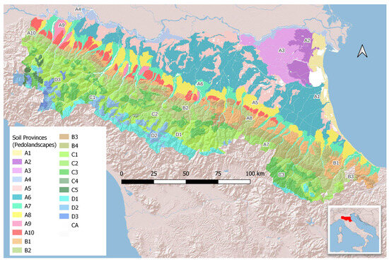
Figure 1.
Study area: Soil provinces of Emilia-Romagna. A1—soils of the coastal plain and delta front; A2—soils in the lower abandoned Po delta plain (Holocene); A3—soils in the upper abandoned Po delta plain (Holocene); A4—soils in the Po meander plain (Holocene); A5—soils in morphologically depressed areas of the lower Apennine alluvial plain; A6—soils of the levees and transition areas of the lower Apennine alluvial plain; A7—soils in the fans and terraces of the upper Apennine alluvial plain (Holocene); A8—soils in the fans and terraces of the upper Apennine alluvial plain (Holocene); A9—soils in the terraced fans of the upper Apennine alluvial plain, located near the main river channels; A10—soils in morphologically high areas of the ancient plain—Apennine fringe (Pleistocene); B1—soils of the lower Apennines of Pliocene clays and sands; B2—lower Apennine soils on unstable clays; B3—lower Apennine soils on mudstones and sandstones; B4—lower Apennine soils on the Marnosa Arenacea Romagnola (turbiditic marly sandstones); C1—soils of the middle Apennines on unstable clays; C2—soils of the middle Apennines on calcareous–marly flysch; C3—soils of the middle Apennines on arenaceous–pelitic flysch; C4—soils of the middle Apennines on gypsum and limestones; C5—soils of the middle Apennines on ophiolitic rocks; D1—soils of the upper Apennines on sandstones; D2—soils of the upper Apennines on calcareous–marly flysch and mudstones—D3—soils of the upper Apennines on ophiolitic rocks.
The Apennines (the highest elevation in Emilia-Romagna at 2165 m a.s.l.) are a typically polyphasic chain of plates, developed over a period that goes from the Cretaceous to the present, following the collision between two continental blocks, the European plate (or Sardinian–Corsican) and the Padano–Adriatic microplate (or Adria), initially connected to the African plate. The collision process between these two continental plates was preceded by the closure of an oceanic area interposed between them, the Ligurian–Piedmont paleocean. The chain thus derives from the complex deformation and eastward superimposition of the sediments deposited in the different Meso–Cenozoic paleogeographic domains: (i) the Ligurian Domain, corresponding largely to the oceanic area, consisting of tectonic mixes and olistostromes with a dominant clay material; (ii) the Epi-Ligurian Domain, which is established starting from the Middle Eocene on the Ligurian units already tectonized, and consisting of thick series of calcareous or arenaceous turbidites, clay breccias, and olistostromes; (iii) the Sub-Ligurian Domain, developed on the thinned African crust adjacent to the oceanic area, represented by pelitic and evaporitic deposits (gypsum), marine clays, and alternating marine conglomerates and sands, (iv) the Tuscan–Umbrian Domain, characterized by strongly cemented turbiditic marly sandstones.
The variety of parent materials and terrain morphologies occurring in the Apennines results in twelve distinct pedolandscapes, which can be grouped based on elevation ranges, i.e., soils of the low (150–450 m a.s.l.), medium (450–900 m a.s.l.) and high (>900 m a.s.l.) Apennines.
The plain area of the region (lowest elevation −8 m b.s.l.) is represented by alluvial materials which filled a subsiding geosyncline and covered the substrate of coastal marine clays, reaching overall thicknesses of up to 300–400 m. In particular, the most recent Pleistocene–Holocene filling deposits have two different sources, i.e., the Po River delta system and the Apennine river systems. The former has dominant W–E axial feeding, while the latter have a dominant SW–NE transverse feeding. The combination of the two depositional systems resulted in a remarkably complex geomorphological pattern of alluvial fans, terraced, fluvial, deltaic, and coastal deposits, where ten different pedolandscapes are identified. Figure 1 illustrates the geographical distribution of the different soil provinces, or pedolandscapes, at the 1: 1,000,000 scale. A soil province is a geographical area defined by relatively uniform soil characteristics, which are influenced by a relatively uniform combination of climate, vegetation, and parent material. A brief description of the dominant soils occurring in each pedolandscape is given in the Supplementary Materials (Table S1).
Due to the different types of terrain and habitats present in the region, and thanks to the presence of the Adriatic Sea, which mitigates the temperature extremes, the climate is not the same in all parts of Emilia-Romagna. In the mountainous area the climate is temperate (Köppen–Geiger Cfb), with rainy summers followed by cold winters, while on the plain, the climate is temperate subcontinental with hot summers (Köppen–Geiger Cfa). The average temperatures of Emilia-Romagna for the twenty-five-year reference period 1991–2015 is equal to 12.8 °C with a minimum in January (0.4 °C) and a maximum in July (27 °C). The average yearly cumulated rainfall for the same reference period amounts to 927 mm, with a maximum of 1957 mm along the northwestern ridge of the Apennines and a minimum of 616 mm in the Po River delta [50].
The land use in Emilia-Romagna is strongly polarized between the highly intensively cultivated plain and the extensively managed mountain rangelands and forests, characterizing 25 agricultural districts: 9 in the alluvial plain, 8 in the low Apennines, and 8 in the medium and high Apennines (Figure 2). In the plains the soils favor intensive agricultural production that, depending on local climate, is characterized by typical Mediterranean crops (orchards, vineyards, and vegetables), cereals, and industrial crops in the eastern plains, to more temperate climate productions such as pasture cereals and pig and dairy farming in the western plains. In the Apennines, more than 60% of the area is broadleaf woodland, with a dominance of oaks (Quercus L.), hornbeams (Carpinus L.), and chestnuts (Castanea sativa Mill.); croplands, grasslands, and permanent crop, respectively, make up 22, 7 and, 3% of the mountain areas.
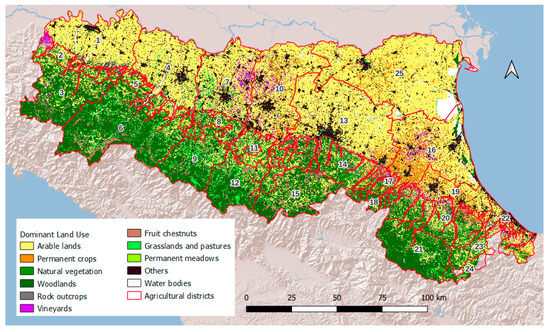
Figure 2.
Dominant land use and agricultural districts (1–25) of Emilia-Romagna. Districts 1 to 14 are in Emilia; districts 16–24 are in Romagna. District 25 is the Ferrara plain.
2.2. Soil Data
The soil property data at the base of the SES assessment, i.e., sand, silt, and clay contents (USDA limits), the percentage of coarse fragments (diameter > 2 mm), pH, organic carbon (C org.) content, and the Soil Biological Quality index (QBS-ar), all for the reference depth 0–30 cm, were provided by the regional Geology, Soil and Seismic Risk Service of Emilia-Romagna. The descriptive statistics of the soil properties are summarized in Table 1. Except for the QBS-ar data, which is characterized by few hundreds of data points, the overall sampling density (observation per km2) ranges from 1.2 to 2.4, coherent then with a 1:50,000 scale, but the data point in the plain area of the region represents 67 to 84% of the total, depending on the property considered. This would suggest that different DSM should be implemented to tackle such a difference in data availability in the two parts of the region.

Table 1.
Descriptive statistics of basic soil properties for the plain and the mountainous areas of Emilia-Romagna.
Additionally, the following thematic maps were provided to support the DSM approaches and the SES mapping: (i) the soil map at 1:50,000 scale, covering 78% of the region (plain, hill, and part of the mountain territory) with the associated soil catalog [51], (ii) the regional soil map at 1:250,000 scale, covering the entire regional territory, (iii) the map of the pedolandscapes (soil provinces, Figure 1), covering the entire region; (iv) the Land Capability Map which classifies the regional soils into eight classes of decreasing suitability for agricultural production (the first four) and forestry or grazing (the last four) [52]; (v) the actual and potential soil erosion maps along with the Revised Universal Soil Loss Equation (RUSLE) factors used for their assessment [53]; (vi) the map of the depth of the shallow groundwater (annual average and seasonal averages) of the plain [54].
As the pedolandscapes describe the regional soil geography, delineating areas where soils are similar in terms of climate, topography, parent material, and vegetation, they represent a useful reference to analyze results in terms of SES supply. For this reason, and to highlight the relevance of soil properties on the definition of SES considered in this work, Table 2 and Table 3 reports for the plain and the Apennines, respectively, the descriptive statistics for the basic soil properties observed in the pedolandscapes of the region.
Table 2.
Descriptive statistics of basic soil properties for the pedolandscapes of the plain area of Emilia-Romagna.
Table 3.
Descriptive statistics of basic soil properties for the pedolandscapes of the mountainous area of Emilia-Romagna.
2.3. Soil Functions and SES Assessment
Soil-based ecosystem services were assessed via indicators based on measured or estimated soil properties which were assumed to be proxies of soil functions, following the methodology described in detail by Calzolari et al. [24]. The method considers a set of indicators of soil functions associated with the potential ecosystem services supply. Although time invariant, the spatially explicit indicator scores allow the ranking of the different soils in terms of their potential ecosystem services supply, based on routinely available soil data. The ecosystem services, the underpinning soil functions, and the soil data required as input for their calculation are presented and fully described in Table 4.
Table 4.
Ecosystem services (ESs), underpinning soil functions, indicators, and input data.
Table 5 reports the computations to derive each indicator, as specified by Calzolari et al. [24], for all the indicators reported in Table 2, except for BIO, BIOMASS, and ERSCRL. The first was derived by applying a digital soil mapping (DSM) technique based on machine learning (ML) algorithms [58] to the set of Soil Biological Quality index values QBS-ar [59] available at regional scale, while the second was based on the standardized value of the median Normalized Difference Vegetation Index (NDVI) [60] resulting from Landsat8 using Google Earth Engine [61] for the reference years 2016–2020. As for ERSCRL, its calculation used the values of potential and actual soil erosion loss due to surface water erosion estimated for the whole region with the Revised Universal Soil Loss Equation applied at 20 m resolution [53].
Table 5.
Input data and calculations of soil ecosystem service (SESs) indicators (0–30 cm).
The Land Capability Classes (LCCs), as originally evaluated for agricultural and forest lands [5], were based on available soil maps at different scales in the plain and in the mountain part of the region. The full list of the LCCs and associated scores for the indicator of potential food provision (PRO) is provided in the Supplementary Material (Table S2). The physical soil properties listed in Table 2, namely BD (bulk density, Mg/m3), Ksat (saturated hydraulic conductivity, mm/hr), PSIe (air entry potential, cm), and WCFC (water content at field capacity, vol/vol) were estimated using locally calibrated pedotransfer functions (PTFs) [62,63,64]. The average shallow groundwater depth WT (cm) was derived from Calzolari and Ungaro (2012) [54]. The estimated SES indicators were finally provided as numbers between 0 and 1 applying an interval normalization transformation as follows [65]:
where Xi0–1 is the normalized value [0–1], Xi is the estimated indicator value, and Xmin and Xmax are, respectively, the maximum and minimum of the indicator in the study area. The maximum observed value is set equal to 1, and the value 0 indicates the relative minimum in the study area. Indicator values are then greatly determined by the range of the measured and estimated soil properties at the scale of investigation. When considering specific parts of a territory of administrative, planning, or management relevance (e.g., province, union of municipalities, municipality), the indicators can be normalized over the area of interest accounting then for the local soil variability.
Xi0–1 = (Xi − Xmin)/(Xmax−Xmin)
2.4. Mapping Soil Properties and Ecosystem Services at Regional Scale
The DSM of basic soil properties at 100 m resolution, preliminary to the SES indicators assessment and mapping, followed two distinct approaches for the plain (1,195,263 ha) and the mountain area (1,057,612 ha) of the region. This was due to the different data availability, both in terms of point data numerosity and thematic map resolution, and to the role that environmental drivers play in determining the spatial patterns of soil properties. In both cases, the target variables for the 0–30 cm reference depth were sand, silt, and clay contents (%), coarse fragments (skeleton, %), organic carbon (%), and pH, In the following subsections the steps of the two approaches are briefly described.
2.4.1. DSM of Soil Properties in the Emilia-Romagna Plain
In the plain area of Emilia-Romagna, a geostatistical simulation approach conditional on the 1:50,000 soil map delineations was used. The spatialization procedure followed, which is one of the possible variants of scorpan kriging [66], returns N simulated values in each 100 × 100 m cell of the estimation grid. The set of simulated values therefore provides a series of N equiprobable representations (maps) whose descriptive statistics calculated in each grid cell also provide not only an average value but also indications on the uncertainty of the estimated data. The geostatistical simulation approach was then implemented through the following steps:
1. Calculation of the weighted average values of the target soil variables (Table 1) for each 1:50,000 soil map delineation (n = 2230) as a function of the percentages of occurrence of each different soil type within the single delineation by using the benchmark soil profile data [63] for the 0–30 cm reference depth (n = 2279).
2. Descriptive statistical analysis, calculation of the residues from the average value for each point observation, and normal score transformation of the residuals.
3. Experimental variography of the normalized residues and modeling of the experimental variograms.
4. Sequential Gaussian Simulations (SGSs) with ordinary kriging of the normalized residues on a regular 100 m grid, back-transformation of the estimated mean residual values (n = 25) and sum of the average value attributed to the 1 ha grid cell and control on the ranges of the obtained values.
5. Map of the estimated value of the target variable and of the cartographic accuracy index; this is defined based on the standard deviation of the simulated values (n = 25) in each cell of the 100 m estimation grid.
All the steps described above, except the third and the last one, were carried out with the WinGSLib software v1.3. [67] that uses the executables of the GSLIB Fortran library [68]. The modeling of the experimental semivariogram was performed by compiling an R script that uses the ‘gstat’ library version 2.0-9 [69,70].
2.4.2. DSM of Soil Properties in the Emilia-Romagna Apennines
For the estimation and mapping of the basic properties of the soil of the Apennines, a DSM approach based on machine learning (ML) algorithms was chosen. This was due to the lower data availability in the Apennine area and to their nonhomogeneous distribution throughout the region. Therefore, we took advantage of the contribution that the so-called environmental covariates can bring to the estimation process. As the covariates were derived from different sources, as illustrated in Table 6, they were all harmonized at 100 m resolution, after reprojection into the same reference system (EPSG:7791).
Table 6.
List of the covariates used in the DSM of the Emilia-Romagna Apennines to estimate basic soil properties. SCORPAN factors: C, climate; O, organisms; P, parent material; R, relief; S, soil (measured properties of the soil at a point).
The models were run in an R environment [71], adapting the DSM workflow developed by the FAO [72] using Quantile Random Forests (QRFs) [73,74]. QRFs deliver a multivariate quantile regression forest along with its conditional quantiles and density values. Each forest ensemble was composed of 500 regression trees, and for each ensemble an extractor function for variable importance measures was applied based on the total decrease in node impurities from splitting on the variable, averaged over all trees. This allowed us to assess the predictive power of each variable. In QRFs, the importance of individual predictors is defined in terms of “node purity,” that is, the homogeneity of the data contained within each node resulting from the subdivision of the data based on the values of a certain variable used as a predictor. The index is in fact calculated as the difference in terms of the rooted mean squared error (RMSE) before and after the division performed on that given variable.
Initially, using the same R scripts, the data sets of each variable were randomly divided into a train and a test set, with, respectively, 75% of the data used for SGS implementation and QRFs calibration and 25% of the data kept for map validation. The script performs a 10-fold cross-validation, splitting the training data set into subsets and using nine subsets for calibration and one subset for validation. This process is repeated 10 times, with a different subset used at each iteration. Calibration and validation errors of the mapped values were eventually assessed by calculating mean error (ME), absolute error (AE), rooted mean squared error (RMSE), index of agreement (IoA), and R2. The IoA [75] is a standardized measure of the degree of model prediction error which varies between 0 and 1, and is calculated as follows:
where Oi is the observation value, Pi is the predicted value, and is the average observation value. The index of agreement represents the ratio of the mean square error and the potential error. The agreement value of 1 indicates a perfect match, and 0 indicates no agreement at all. The index of agreement can detect additive and proportional differences in the observed and simulated means and variances; however, IoA is overly sensitive to extreme values due to the squared differences.
For the post processing of the combined results of the two areas of the region in terms of the potential contribution of SES provision at regional scale, the 22 functionally distinct pedolandscapes based on the Emilia-Romagna Soil Map at scale 1:50,000 [51] were considered. Examples of the application of the SES maps to support spatial planning on a local scale, i.e., municipality, are also presented.
3. Results and Discussion
3.1. Maps of Basic and Derived Soil Properties
The assessment of the indicators of ecosystem services followed the mapping of the necessary chemical–physical parameters over the 100 m estimation grid. For this purpose, the point data values in the plain area of Emilia-Romagna were interpolated with geostatistical simulations conditional on the means of the soil map polygons to reconstruct the continuous spatial distribution of the parameters reported in Table 1. This was followed by the pedotransfer estimation of physico-chemical soil properties.
Table 7 reports the parameters of the semivariogram models (Figure S1) used for the spatial interpolation of the normalized residuals of the three textural soil fractions, pH, and organic C content. A double spherical model with nugget provided the best interpolation of the experimental semivariograms for all soil variables. The normalized residuals of the soil properties have a spatially uncorrelated variance (nugget, C0) ranging between 17 and 23% of the total variance. The short-range sill component C1 accounted for almost 70% of the residual variance in the case of the three textural fractions, while for pH and organic C content the long-range sill component C2 explained up to 38 and 44%, respectively, of the spatially structured variance.
Table 7.
Parameters of the semivariogram models for selected soil properties. For all properties, the parameters refer to double nested spherical models. The spherical semivariogram model can be written as follows: γ(h) = C0 + Σni=1 Ci(1.5 h/ri − 0.5 h3/ri3), for h ≤ ri, where h is the distance (m), C0 is the nugget, Ci (i = 1, …, n) the sill of the i nested structure, and ri its spatial range (m).
Differently from the spatial autoregressive approach underpinning the implementation of geostatistical SGSs in the plain area, the DSM procedure followed for the hilly and mountainous area allowed us to identify the relevance of the covariates used as predictors in calibrating the QRFs. Figure 3 illustrates the relevance of the different covariates in terms of node purity; to plot the five soil properties considered together, the node purity values were standardized to the same 0–1 range. The 23 covariates on the Y axis of the bar plot are in decreasing order of importance based on their average ranks and can be separated into five groups: (i) climate covariates (n = 1), (ii) topography covariates (n = 9), (iii) land use land cover covariates (n = 4), (iv) soil covariates (n = 4), (v) surface reflectance covariates (n = 5). The climate covariate, i.e., the long-term average temperature of the warmest month, ranked first in terms of importance for predicting organic carbon content, followed by elevation and average C org content per land use class at agricultural district level. This is the only case in which climate and land use rank high as predictors, as the other soil properties considered appear far less relevant. The limited role played by land use and land cover covariates (mean rank > 11) might in part be due to the spectral reflectance covariates, which have an intermediate relevance as predictors, particularly the NDVI (mean rank 4) and the EVI (mean rank 8) which greatly outperformed the relevance of the topography covariates (mean ranks > 9) with the sole exception of elevation (mean rank 3). In addition to C org. content, elevation ranked second in terms of relevance in the case of silt content, skeleton %, and pH, while its relevance ranked fifth for both sand and clay contents. Apart from C org. content, the soil covariates were those with the highest relevance, with the average content per map polygon ranking first for all textural fractions and skeleton content, while the categorical variables referring to the pedolandscapes of the Apennines and to the classed average contents of sand and clay ranked on average fifth and sixth, respectively. Soil erosion also exhibited a high relevance, ranking third for silt content, and having a mean rank of seven. The relevant role played by the covariates related to soil geography was observed also for the skeleton content of the plain for which a DSM approach based on QRFs was adopted as well: in this case the first three covariates in terms of predictive relevance were the mean content of coarse fragments of the 1:50,000 soil map polygons, and the two categorical covariates expressing the mapping units of the 1:250,000 and the 1:50,000 soil maps of the plain.
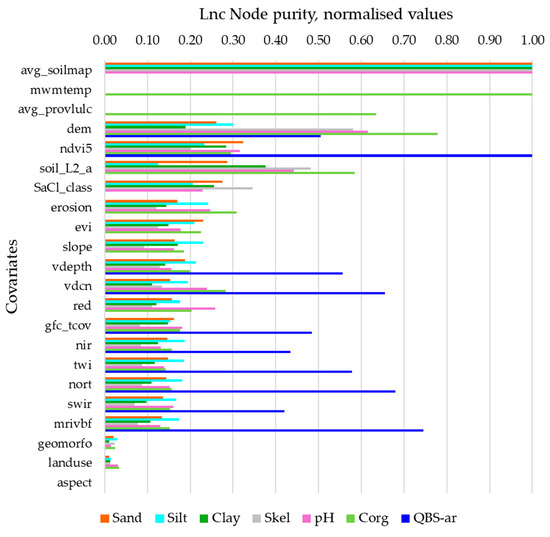
Figure 3.
Importance of the covariates for modeling soil properties by QRFs in the hilly and mountainous area of Emilia-Romagna.
Table 8 reports the error indices for the validation and calibration datasets of the basic soil properties for which maps at 100 m resolution were derived using the approaches outlined in Section 2.4.1 and Section 2.4.2.
Table 8.
Error indices for calibration and validation data sets.
Based on test error statistics, the best predicted variable was the C org. content, in both areas, whilst skeleton content in the plain and the pH in the Apennines were less predictable. Among the textural fractions, clay content was the best predicted in the plain while it was the worst predicted in the Apennines. On average, the predictions were more accurate for the plain than for the Apennines, which comes as no surprise given the size of the two data sets. Nevertheless, the performance metrics of both DSM approaches are good. The resulting maps are displayed in Figure 4a–f. The maps of the spatial uncertainty for the six estimated soil properties are displayed in the Supplementary Materials (Figure S2).
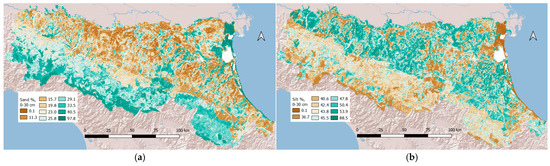
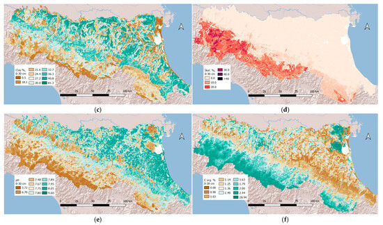
Figure 4.
Raster maps (resolution 100 m) of basic soil properties (0–30 cm): (a) sand %, (b) silt %, (c) clay %, (d) coarse fragments %, (e) pH, (f) organic C %. The classes in the map legends are based on the deciles of the observed distributions, except for coarse fragment content, for which an equal interval legend was selected.
At the nodes of a 100 m regular grid over the entire region, a set of locally calibrated pedotransfer functions assessed the values of the soil properties requested to calculate the indicators for the selected SESs. The PTF-estimated properties were bulk density (BD, Mg m−3), which was necessary to calculate soil C stock (Mg/ha, for the reference 0–30 cm depth), hydraulic conductivity at saturation (Ksat, mm h−1), air entry tension (PSIe, cm), water content at field capacity (WCFC, vol./vol.), and cation exchange capacity (cmol/kg). The raster maps of the PTF-derived soil properties are shown in Figure 5a–f.
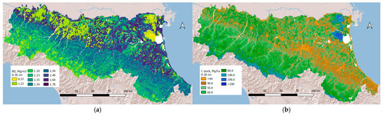
Figure 5.
Raster maps (100 m resolution) of PTF-derived soil properties (0–30 cm): (a) bulk density (Mg/m3), (b) organic C stock (Mg/ha), (c) water content at field capacity (vol./vol.), (d) cation exchange capacity (cmol/kg), (e) saturated hydraulic conductivity (mm/h), (f) air entry tension (cm).
3.2. Maps of Soil-Based Ecosystem Services at Regional Scale
The resulting maps of the eight indicators of SESs considered are shown in Figure 6a–h. All indicators were normalized on the observed variability (minimum and maximum values) at the regional scale in order to have values between zero and one for all indicators. The raster maps have a resolution of 100 m and cover the entire region. In the case of potential food provision, the indicator PRO was based on the 0–1 normalization of the LC classes mapped at the regional scale [52]; both the LCC map and LC standardized values are provided in the Supplementary Materials, in Figure S3 and Table S2, respectively. The values of the indicators displayed in the maps in Figure 6 were eventually post processed to characterize the potential ecosystem services provision in the 22 soil provinces of the region. The descriptive statistics of each indicator for the different cartographic units of the pedolandscapes map (Figure 1) were eventually used to assess the synergies and trade-offs among services, returning the figures shown in Table 9 and graphically summarized by the radar charts in Figure 7.
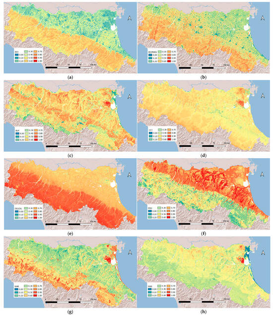
Figure 6.
Raster maps (100 m resolution) of soil-based ecosystem services (0–30 cm): (a) habitat for soil organisms (BIO), (b) biomass production (BIOMASS), (c) buffering capacity (BUF), (d) carbon sequestration (CST), (e) erosion control (ERSCRL), (f) food provision (PRO), (g) water regulation (WAR), (h) water storage (WAS).
Table 9.
Average values of SESs indicators for the mapping units of the pedolandscapes (soil provinces) map of Emilia-Romagna.
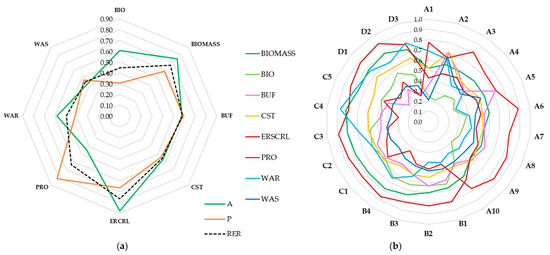
Figure 7.
Mean values of the eight SESs indicators in plains, the Apennines, and the whole region (a), and in the pedolandscape units of Emilia-Romagna (b).
The data reported in Table 9 highlight a marked distinction in SES potential supply of the different pedolandscapes of the region, as can be visually appreciated in Figure 7. In general, clear contrasts were observed between the soil provinces of the plains and those of the Apennines, with the former outperforming the latter only in terms of potential food supply by 31%. On the other hand, in the Apennines the potential supply of habitat for soil organisms and biomass provision was well above the regional mean by 36 and 13%, respectively (Figure 7a). Similar differences were observed for the regulating services WAR and ERSCRL, which are above the regional mean by 14 and 18% respectively. As for the other regulating service indicators, BUF and WAS had very similar mean values across the two landscapes, with the plains exhibiting slightly high values with respect to the Apennines by nearly 2 and 5%, respectively. Quite surprisingly given the striking differences in land use intensity, the potential carbon sequestration regulating service was very similar with mean values being higher and lower than the regional average by ca. 2.5% in the Apennines and in the plains, respectively (Figure 7a).
Table 10 reports the correlation coefficients between the average values of the ecosystem service indicators of the mapping units of the pedolandscapes map. From the data in the table, based on the trends of the mean values depicted in Figure 7b, it can be seen that in most cases, the services were synergic with each other: positive significant correlations were observed for BIO and BIOMASS, BIO and BIOMASS and ERSCRL, WAR and ERSCRL, WAR and BIOMASS, and BUF and WAS. Clear trade-offs with significant negative correlations characterized WAR and WAS, WAR and BUF, and nearly all the correlations between PRO and the other services, except for BUF, with which there was significant synergy.
Table 10.
Pearson’s correlation coefficients between the mean values of the SES indicators of the soil provinces. Statistically significant correlations are in bold (p = 0.05).
Further insights into these trends and their spatial patterns can be gained in the following subsections, where results for specific SES in the different pedolandscape units summarized in Figure 7b are presented and discussed.
3.2.1. Buffering Capacity (BUF)
The soil buffering capacity (BUF) in Emilia-Romagna’s plains and the Apennines varies significantly with texture, coarse fragment content, cation exchange capacity, and pH. In the plains, BUF is highest in clay-rich, alkaline soils of the low alluvial plain’s depressed areas (unit A5) and parts of the delta plain (unit A2), but very low in the coastal plain (unit A1) and in parts of the Po meandering plain (unit A4), due to the presence of sandy soils. Desaturated soils along the western Apennine margin (unit A10) also exhibit a low BUF due to acidic topsoils (pH < 6.5). A moderate BUF dominates elsewhere in the plains, though coarse-textured soils in the levees (unit A6) and the upper delta plain (unit A3) have a reduced buffering capacity.
In the lower Apennines, BUF ranges from moderate–high in fine-textured, high-pH units (B1, B2) to low in coarser, skeletal, or acidic soils (units B3 and B4). The medium Apennines show greater variability due to heterogeneous soil textures, landslide-prone clays (unit C1), and acidic soil under woodlands. BUF is moderately low in soils derived from calcareous–marly flysch (C2) in the eastern part of the chain but higher in finer soils in the western part, while coarse-textured or gypsum-derived soils (C3, C4) have a very low buffering capacity. Ophiolitic soils (C5) are mixed, with a low BUF in skeletal soils but a moderate capacity where finer textures prevail. In the upper Apennines, the protective capacity is generally low or very low in units D1 and D3, due to the presence of coarse-textured, skeletal, and acid soils; in unit D2 it is somewhat higher due to soils with medium or fine textures and with a higher pH.
3.2.2. Carbon Sequestration (CST)
This indicator (Figure 6d) is based on the estimated carbon stock (Mg/ha) for a reference depth of 30 cm (Figure 5b). The average organic carbon stock of topsoil (0–30 cm) is 59.9 Mg/ha (SD 30.9 Mg/ha) across the region, with distinct variations between the plains and the Apennines. The plains exhibit lower average stocks (52.5 Mg/ha, SD 32.6 Mg/ha) compared with the Apennines (66.3 Mg/ha SD 24.6 Mg/ha), peaking in Ferrara’s peaty delta soils of soil province A2 (148.1 Mg/ha, SD 66.7 Mg/ha) and forage-rich agricultural districts of Parma and Reggio Emilia (ca. 58 Mg/ha). Conversely, the lowest stocks occur in the sandy soils of the coastal and meander plain (ca. 43–45 Mg/ha) and desaturated soils near the Apennine fringe (as low as 30.8 Mg/ha), exacerbated by land use changes towards intensive orchard expansion. In the Apennines, carbon stocks rise with elevation: at the lower elevations they reach an average value of 48.0 Mg/ha with the lowest value in the soils of the B1 unit on Pliocene sands/clays (42 Mg/ha, SD 17.4 Mg/ha), with mid-elevation soils reaching 71.3 Mg/ha (SD 13.1 Mg/ha) and peaking in soils of unit C5 on ophiolitic rocks at 76.8 Mg/ha (SD 15.7 Mg/ha), while higher area soils attain 106.6 Mg/ha (SD 20.6 Mg/ha) with an average maximum stock in soils on sandstones (unit D1) with 113.9 Mg/ha (SD 24.0 Mg/ha).
3.2.3. Food Production (PRO)
The soil capacity to sustain food production in Emilia-Romagna was evaluated using the Land Capability Classification (LCC) system, revealing a clear dichotomy between plains and Apennine areas. The plains (52% of the region) predominantly contain highly productive LCC Class I–III soils (PRO scores 1.0–0.714), with 58% of the area exhibiting few to moderate limitations (Classes I/II/II–I), particularly in pedolandscape units A6 and A9. The delta plain (unit A2) represents an exception, containing Class IV soils with an average PRO score of 0.65. Approximately 24% of plains soils face severe limitations (Classes III–IV/VI, PRO 0.714–0.443), while 4% are unsuitable for agriculture (Class V, PRO 0.429). In contrast, the Apennines are dominated by Classes III–VIII, with Class II soils only located in intra-valley terraces. The most prevalent classes are VI (PRO 0.286) and III (PRO 0.70) and their intergrades (VI/III, III/VI; PRO 0.479–0.521), summing up to 54% of mountain soils and occurring primarily in units C1, C5, B2 and D2 (PRO > 0.45). Intermediate classes (31% coverage, PRO 0.45–0.35) dominate units B1, B3, C3 and D1, while Class VI/VII soils (PRO < 0.35) prevail in wooded areas of units B4, C4 and D3. This spatial distribution reflects the combined influence of natural soil constraints (slope, texture, coarse fragments content, drainage) and anthropogenic modifications, with the plains supporting intensive agriculture while the Apennines exhibit progressively reduced production potential corresponding to elevation-driven pedogenic gradients.
3.2.4. Water Regulation (WAR)
The infiltration process is regulated primarily by three soil parameters: the saturated hydraulic conductivity (Ksat, mm h−1), the pore size distribution, and the saturation conditions of the soil. In the indicator-based approach presented in this work, the first two parameters were accounted for, and the variability of water infiltration capacity of soils reflects the variability of the above-mentioned parameters at regional scale (Figure 6g) with distinct spatial patterns tied to soil texture and lithology.
In the plain, infiltration capacity is highest in coastal sandy soils (unit A1) and organic carbon-rich deltaic soils, followed by sandy deposits of the Po meandering plain (unit A4), Romagna’s river levees (unit A6), and portions of the upper delta plain (unit A3). Moderately low WAR occurs in transition zones between levees and depressions of the low alluvial plain (unit A6) and in alluvial fans and river terraces (units A7 and A8) where silty-textured soils dominate. The lowest infiltration capacity characterizes clay-rich depressed areas of the low alluvial plain (unit A5), portions of the upper delta (unit A3), and fine-textured Apennine margin soils (unit A10).
Apennine soils show an elevation-dependent trend, with WAR increasing from the lower to upper zones. The lower Apennines display minimal infiltration in fine-textured soils of units B1 and B2, moderate capacity in unit B3 soils, and higher values in marly sandstone-derived soils (unit B4). Middle Apennine units exhibit uniformly moderately high to high WAR indicator scores, progressing from unstable clays (unit C1) to gypsum/limestone (unit C4) and ophiolitic soils (unit C5), the latter two showing comparable peak performance. This spatial variability reflects the primary control of lithology on soil texture, with secondary influences from geomorphic position (ridge vs. depression) and organic matter content, creating a clear gradient from restricted drainage in clay-dominated lowlands to optimal infiltration in coarse-textured uplands.
3.2.5. Water Content at Field Capacity (WAS)
This indicator is based on the water content at field capacity for the reference depth interval of 0–30 cm, corrected for the content of coarse fragments and the possible presence of a shallow water table within the reference interval considered. Although the soil water potential at field capacity depends on soil type, the WAS indicator is based on the estimated water content at the reference tension of −33 kPa, as recommended in the absence of field measurements [76]. The water storage capacity (WAS) of soils is primarily governed by granulometric grain size characteristics, organic matter content, and depth, exhibiting an inverse relationship with water regulation (WAR) capacity in mineral soils, while organic soils maintain high values for both SESs. Clayey and silty soils, particularly when organic carbon-rich, demonstrate superior water retention, while coarser-textured soils show limited storage potential (Figure 6h).
In the plains, minimal WAS occurs in coastal sandy soils (unit A1), contrasting with maximal values in clay-rich (>60% clay) depressed areas of the lower alluvial plain (unit A5, agricultural districts 7, 10, and 13). A moderately high capacity characterizes transition zone soils of the lower alluvial plain (unit A6), clayey soils of the delta plain (unit A2), and silt/clay-dominated soils of fans/terraces of the upper alluvial plain (units A7 and A8). Reduced water storage prevails in coarser-textured soils of the Po meandering plain (unit A3) and gravelly deposits of alluvial fans and terraces (units A7 and A9).
The Apennines exhibit progressive storage limitations with elevation. The lower Apennine units show a moderate capacity in clayey soils (B1–B2) but moderately low values in pelitic sandstone (B3) and marly sandstone (B4) units, particularly in coarse-textured Pliocene deposits (B1, agricultural districts 2 and 14). Middle Apennine pedolandscapes display the lowest WAS in gypsum/limestone (unit C4), unstable clays (Unit C1), and ophiolites (unit C5), with moderately low values in soils derived from arenaceous–pelitic flysch (unit C3) and calcareous–marly flysch (unit C2) soils. Upper Apennine units maintain a limited storage capacity, being lowest in soils derived from sandstones (unit D1) and ophiolites (unit D3), and moderately low in calcareous–marly flysch/mudstones (unit D2). This spatial distribution underscores lithology as the primary control on texture-dependent water retention, modified locally by organic matter accumulation and geomorphic position.
3.2.6. Biomass Provision (BIOMASS)
Since PRO is an indicator of potential soil productivity based on limitations on use, it was proposed to support it with an indicator of biomass production estimated by spectral indices derived from satellite images and based on the normalization of mean yearly median NDVI (Normalized Difference Vegetation Index, Landsat8, 30 m resolution) values between 2015 and 2020 (Figure 6b). This provisioning service is particularly relevant in the Apennine area, as it assumes the highest values in woods, shrubs, and permanent meadows, as well as orchards and vineyards, especially in the plains and hilly areas. In fact, it compensates for the less than exceptional performance of the PRO indicator in the mountains and hills. It assumes a value of zero in the absence of vegetation (soil-sealed areas, rivers and water, or rocky outcrops). The patterns observed on the indicator map mirror the density of the vegetation cover as determined by the dominant land use.
3.2.7. Habitat for Soil Organisms (BIO)
The BIO indicator scores were derived by spatializing and normalizing the range of estimated values of the QBS-ar values with DSM techniques, testing the effectiveness of categorical and continuous predictors such as land use, vegetation indices from remote sensing, altitude, and other indices derived from the DEM and soil variables (e.g., textural fractions, organic C content, and water content at field capacity and at the wilting point).
Despite the good validation statistics, given the limited number of QBS-ar data available at regional level, the BIO indicator map is to be considered as a preliminary description at regional level but with little applicability at local scale. However, the machine learning algorithms underlying the DSM have highlighted the relevance of remote sensing vegetation spectral indices as predictors of QBS-ar, offering a provisional map that could be the basis for validating hypotheses on the drivers that determine the spatial distribution of the BIO indicator at the regional scale.
In general, the BIO indicator for a large part of the Emilia-Romagna plain is moderately low to very low. The lowest value is in urban areas, a little higher in arable land that is widely spread, with minimums in the Rimini (agricultural district 22) and Ferrara (agricultural district 25) plains, while moderate and moderately high values characterize the grassed orchards of Romagna and Modena. The value of the indicator is also moderate in the Parma and Reggio plain (agricultural districts 4 and 7) area due to the widespread presence of forage crops. Another exception is the residual woodlands along the Apennine margin (unit A10). Moderately high to high values characterize a large part of the Emilia-Romagna Apennines, with higher indicator scores in the hilly area compared with the mountainous area in agreement with a negative trend with elevation.
3.2.8. Erosion Control (ERSCRL)
This regulation service is calculated based on the difference between potential erosion (Mg ha−1 yr−1) and actual erosion (Mg ha−1 yr−1). The effect of soil cover is set to zero to calculate potential erosion, considering how it affects potentially bare soil. As such, the indicator ERSCRL considers how soil cover, crops, and crop management cause a variation in soil erosion compared with those that would occur in the absence of vegetal cover. As expected, the indicator scores are significantly higher in the Apennines than in the plains, with a positive trend with elevation and a strong significant correlation (R2 = 0.89) with plant biomass as described by the BIOMASS indicator scores for the pedolandscape units (Figure 8).
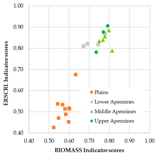
Figure 8.
ERSCRL indicator scores vs. BIOMASS indicator scores.
3.3. Application of the SES Maps to Support Spatial Planning on a Local Scale
Ecosystem service maps were produced at a regional scale, but it is possible to scale the SES indicator scores also at the provincial, union of municipalities, and municipality level by cutting the map along the limits of the chosen administrative unit and recalculating each indicator with Equation (1), except for PRO which is based on the 0–1 scoring of a categorical variable (i.e., the soil LC class). The 0–1 indicator score is not an absolute value but is conditioned by the characteristics of the estimated indicator scores population. By recalculating the indices in the territory of interest it is therefore possible to evaluate, at a local level, the best soils in terms of ecosystem service potential supply. The information resulting from the implementation at local scale of the SES assessment framework presented in this work fulfils the mandatory request to provide soil information and soil-based ecosystem services within the General Urban Plan (PUG) which each municipality of the region has to provide, as requested by the Emilia-Romagna regional law 24/2017 on land planning to reduce and mitigate land take towards the EU target of zero net land take by 2050 [77].
Here we present as examples the results for two municipalities, one in the Ferrara Plains (Portomaggiore, 44°42′ N 11°48′ E, 121.8 km2, agricultural district 25) and one in the upper Bolognese Apennines (Castel di Casio, 44°10′ N 11°02′ E, 46.1 km2, agricultural district 15), whose locations are displayed in Figure 9 and Figure 10, respectively, along with the excerpts of the SES maps at regional scale and the same maps recalibrated on the local variability. In the first case, BIOMASS and ERSPRO services are not shown as they are considered more relevant to the mountain environment. From the maps in Figure 9, it can be appreciated that the change in scale for the interval normalization has a different impact depending on the indicator. For example, in this case the spatial pattern of the WAS indicator at the municipal scale is not very different from that at the regional scale, while for the CST indicator the change in scale in the areas with the lowest carbon stock involves a clear change in the relative values once normalized on the variability range estimated at the municipal level. In all cases though, the interval normalization over the local range resulted in highlighting local minimum and maximum values, with a consequent shift in the whole distribution of the indicator scores.

Figure 9.
Maps of selected ecosystem service indicator scores at regional and local scale in the municipality of Portomaggiore (Ferrara plain, agricultural district 25).
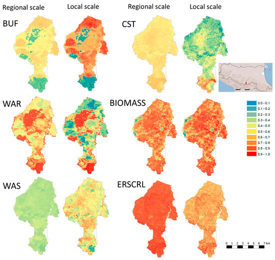
Figure 10.
Maps of selected ecosystem service indicator scores at regional and local scale in the municipality of Castel di Casio (Bolognese Apennine, agricultural district 15).
In the case of the Apennine municipality, the interval normalization over the local range revealed spatial patterns almost undetectable at the regional scale: this is the case of the indicators scores of CST, ERSCRL, and WAS. As for the other indicators in Figure 10, namely BUF, WAR, and BIOMASS, the same spatial patterns evident at regional scale are reproduced at the local scale, but the scores are stretched over a wider range. In this way, local minima and maxima became clearer on the maps, allowing end users to identify more easily the areas of a high and low potential supply of soil-based ecosystem services. In both cases, the spatial patterns of the indicator scores that resulted were more complex, mirroring with further details the underpinning soil variability at a local scale.
Table 11 reports the raster means and the standard deviations of the SES indicator scores in the two municipalities shown in Figure 9 and Figure 10, highlighting the relative changes that occurred in the indicator scores following the 0–1 interval normalization on the local ranges. The relative change in mean values takes different signs depending on whether the local indicator score mean is above (positive difference) or below (negative difference) the mean resulting from the regional normalization. From the standard deviation values in the table, the role played by local variability in affecting the spatial patterns of specific SES indicator scores over the area of interest can be easily appreciated. In both municipalities and for all indicators, there is a systematic increase in indicator score variability when normalized to the local variability ranges.
Table 11.
SES mean indicator scores and their standard deviations (SD) in two municipalities, 0–1 normalized at regional and local scale, and relative differences with respect to the regional scale stemming from the 0–1 normalization with the local ranges.
4. Conclusions
This work illustrated a methodology to enable the regional-scale uptake of soils ecosystem service potential into land planning policies, allowing at the same time an indicator-based assessment of SESs variations due to land use changes. Spatially explicit knowledge of the geography and properties of soils enabled the regional scale implementation of an ecosystem service assessment framework originally developed for agricultural soils of the plains of Emilia-Romagna and now extended to include the hilly and mountainous areas of the region under different land covers at a finer spatial resolution. In doing so, further soil-based ecosystem services were included in the framework to account for the specific conditions of the mountainous area of the region.
The methodology is based on a spatially explicit approach that combines available soil data, locally calibrated pedotransfer functions, and geostatistical or machine learning techniques.
On the one hand, the key strength of this approach lies in its flexibility and capacity to tackle different scales in the case study area; it not only accommodates current land use data and local pedolandscape knowledge but can also integrate new information as it becomes available, ensuring dynamic and up-to-date assessments. Crucially, it clarifies cause-and-effect relationships between land use decisions (e.g., urban expansion, agricultural and forestry practices, and pasture and rangelands management) and SES outcomes, enabling policymakers to quantify trade-offs—such as soil loss versus economic gains—under different scenarios. This is particularly vital in addressing systemic gaps in spatial planning, where SESs are frequently confused with land cover services (e.g., habitat protection in Natura 2000 sites) or overlooked entirely, leading to ineffective policies and exacerbated soil degradation.
On the other hand, a shortcoming in the current modeling methodology is the lack of explicit consideration and assessment of how spatial uncertainties propagate through the SES modeling workflow. This means that DSM models and PTFs produce output in terms of potential SES supply indicators maps, but the reliability and confidence of those indicators, given the inherent uncertainties in inputs and model assumptions, are not quantified. This is a well-acknowledged issue in DSM but very rarely considered in ES modeling [78,79,80]. For some of the SES indicators presented in this work grid-uncertainty maps, which indicate uncertainty directly, could be provided straightforward, as for BIO and BIOMASS using their estimation standard deviations (Figures S4 and S5). For others, though, the uncertainty propagation assessment is more complex and should resort to different post processing techniques depending on input data characteristics. For categorical data, as in the case of PRO, class purity could be assessed using soil map polygon disaggregation techniques, while for continuous data, as for most composite SES indicators presented in this work, uncertainty effects might be additive or multiplicative. It is worth noting that for some authors though, uncertainty assessment would not be strictly required for the indicator-based modeling of ES [81,82,83], particularly when the assessment aims to raise awareness in policymakers and when the focus is on highlighting potential magnitudes and relative rankings, as in the indicator-based approach presented in this work.
When assessing ecosystem services, it is essential to integrate the characteristics of natural capital, in this case soil, with the objectives of prevention, restoration, and management of territorial and urban planning tools. The results highlighted the strong polarization in the types of ecosystem services provided by the soils of the plain and those of the mountain: mainly provisioning services in the former and supporting/regulating services in the latter. As Emilia-Romagna is a region of two distinct parts, it is crucial to enhance and manage the functional interconnections between the plains and the mountains, especially at a time when the consequences of increasingly frequent extreme events—driven by the current climate crisis and shortsighted land use planning—are undermining the flow of benefits associated with ecosystem services. On the one hand, the provisioning services of the best agricultural soils of the plains are constantly eroded by new industrial settlements, logistic infrastructures, and increasingly widespread transport infrastructures, while on the other the regulating services of the mountain soils are jeopardized by a lack of land management and appropriate measures to prevent hydrogeological risks. The mountains are still only seen as a winter playground for the inhabitants of large cities, and the public funds invested in their recreational services for an increasingly short winter season are too often at the expense of the supporting and regulation services that would make it possible to at least partially halt the depopulation dynamics of the mountains.
The study, underscoring the real-world applicability of a soil-based ecosystem service framework, highlights its alignment with legislative efforts like Emilia-Romagna’s Regional Law No. 24/2017, which targets soil consumption reduction by accounting for local soil functionality. To date, 51% of the municipalities in Emilia-Romagna requested from the Regional Soil Services information on the ecosystem services provided by agricultural and forest soils to integrate them into the general urban plans of their territory, showing an ongoing uptake of SES assessment results by decision makers. Such information resulted from the implementation of the SES assessment framework presented in this work to the whole Emilia-Romagna region.
By providing a science-backed, scalable tool, the methodology advocates for soil-centric governance that recognizes soils as multifunctional systems—critical for food security, climate resilience, and biodiversity—rather than mere spatial units.
Supplementary Materials
The following supporting information can be downloaded at: https://www.mdpi.com/article/10.3390/geographies5030039/s1, Table S1. Dominant soils occurring in the pedolandscapes of Emilia-Romagna; Table S2. Land Capability Classes (LCCs) and PRO indicator scores; Figure S1. Experimental (dots) and model (continuous line) semivariograms for the normal score transforms of the residuals of soil properties (0–30 cm); Figure S2. Spatial uncertainty maps of estimated soil properties (0–30 cm); Figure S3. Map of the Land Capability Classes of the soils of Emilia-Romagna; Figure S4. Map of the spatial uncertainty of the indicator BIO; Figure S5. Map of the spatial uncertainty of the indicator BIOMASS.
Author Contributions
Conceptualization, C.C., P.T. and F.U.; methodology, C.C., F.U. and P.T.; software, F.U. and P.T.; validation, P.T. and F.U.; formal analysis, F.U. and C.C.; investigation, F.U., C.C. and P.T.; resources, P.T.; data curation, F.U. and P.T.; writing—original draft preparation, F.U.; writing—review and editing, P.T. and C.C.; visualization, F.U., P.T. and C.C.; supervision, F.U. and P.T.; project administration, F.U. and P.T.; funding acquisition, P.T. All authors have read and agreed to the published version of the manuscript.
Funding
This research was funded by the Emilia-Romagna Region (RER)—General Directorate for Environment and Land Care—Geological, Seismic and Soil Service, grant n. 558 26/04/2021, within the framework of the RER-CNR four-year research agreement “Digital soil mapping applications for ecosystem services assessment and climate change strategy support and knowledge tools to support the EU Nitrates Directive”.
Data Availability Statement
The 1:50,000 soil map of Emilia-Romagna (Ed. 2021) is available via the WMS service at the following link: https://servizigis.regione.emilia-romagna.it/wms/suoli?request=GetCapabilities&service=WMS (accessed on 20 July 2025). The soil map is also available for download at the following link: URL: https://mappegis.regione.emilia-romagna.it/moka/ckan/suolo/Carta_Suoli_50k.zip (accessed on 20 July 2025). The maps of the basic and derived soil properties can be downloaded at the following link: https://datacatalog.regione.emilia-romagna.it/catalogCTA/group/suolo (accessed on 20 July 2025). The maps of soil-based ecosystem services for the whole territory of Emilia-Romagna at 100 m resolution in raster GEO TIF format are available at the following link: https://mappegis.regione.emilia-romagna.it/moka/ckan/suolo/Servizi_ecosistemici_rst.zip (accessed on 20 July 2025). SES indicator maps rescaled at the level of provinces, unions of municipalities, and municipalities, supplemented with a knowledge framework on local soils, are available for the drafting of urban plans (PUG) by sending a request via certified electronic mail to: segrgeol@postacert.regione.emilia-romagna.it.
Acknowledgments
The authors wish to thank the CNR-IBE and RER office staff for all the administrative work and the technical support that allowed the accomplishment of the research activities. The authors wish to thank the two anonymous reviewers whose work provided valuable suggestions to improve the structure and the contents presented in the final version of the paper.
Conflicts of Interest
The authors declare no conflicts of interest.
Abbreviations
The following abbreviations are used in this manuscript:
| BIO | Habitat for Biodiversity |
| BIOMASS | Biomass production |
| BUF | Buffering capacity |
| CLC | CORINE Land Cover |
| CST | Carbon sequestration |
| DSM | Digital soil mapping |
| ERSCRL | Erosion control |
| LCC | Land Capability Class |
| LULC | Land Use Land Cover class |
| MLA | Machine Learning Algorithm |
| NDVI | Normalized Difference Vegetation Index |
| PRO | Food production |
| PTF | Pedotransfer function |
| PUG | General Urban Plan |
| QBSar | Soil Biological Quality |
| QRF | Quantile Random Forest |
| RER | Regione Emilia-Romagna |
| RUSLE | Revised Universal Soil Loss Equation |
| SD | Standard deviation |
| SES | Soil-based ecosystem service |
| SGS | Sequeantial Gaussian Simulation |
| SOM | Soil organic matter |
| WAR | Water regulation |
| WAS | Water storage |
References
- Baveye, P.C.; Baveye, J.; Gowdy, J. Soil “Ecosystem” Services and Natural Capital: Critical Appraisal of Research on Uncertain Ground. Front. Environ. Sci. 2016, 4, 41. [Google Scholar] [CrossRef]
- Costanza, R.; d’Arge, R.; De Groot, R.; Farber, S.; Grasso, M.; Hannon, B.; Limburg, K.; Naeem, M.; O’Neill, R.V.; Paruelo, J.; et al. The value of the world’s ecosystem services and natural capital. Nature 1987, 387, 253–260. [Google Scholar] [CrossRef]
- Costanza, R.; d’Arge, R.; de Groot, R.; Farber, S.; Grasso, M.; Hannon, B.; Limburg, K.; Naeem, S.; O’Neill, R.V.; Paruel, J.; et al. The value of the world’s ecosystem services and natural capital 1. Ecol. Econ. 1998, 25, 3–15. [Google Scholar] [CrossRef]
- MEA. Millenium Ecosystem Assessment, Ecosystem and Human Well-Being: A framework for Assessment; Island Press: Washington, DC, USA, 2005. [Google Scholar]
- Klingebiel, A.A.; Montgomery, P.H. Land-capability classification. Soil Conservation Service. In Agriculture Handbook No. 210; USA Department of Agriculture: Washington, DC, USA, 1961. [Google Scholar]
- FAO. A Framework for Land Evaluation, Soils Bulletin 32; Food and Agricultural Organization of the United Nations: Rome, Italy, 1976. [Google Scholar]
- FAO. Report on the Agro-Ecological Zones project. Volume. 1, Methodology and Results for Africa. In FAO World Soil Resources Report 48/1–4; Food and Agricultural Organization of the United Nations: Rome, Italy, 1978. [Google Scholar]
- FAO. Report on the Agro-Ecological Zones project. Volume 2, Methodology and Results for Southwest Asia. In FAO World Soil Resources Report 48/1–4; Food and Agricultural Organization of the United Nations: Rome, Italy, 1979. [Google Scholar]
- FAO. Report on the Agro-Ecological Zones project. Volume 3, Methodology and Results for South and Central America. In FAO World Soil Resources Report 48/1–4; Food and Agricultural Organization of the United Nations: Rome, Italy, 1980. [Google Scholar]
- FAO. Report on the Agro-Ecological Zones project. Volume 4, Methodology and Results for Southeast Asia. In FAO World Soil Resources Report 48/1–4; Food and Agri-cultural Organization of the United Nations: Rome, Italy, 1981. [Google Scholar]
- Ernstson, H. The social production of ecosystem services: A framework for studying environmental justice and ecological complexity in urbanized landscapes. Landsc. Urban Plan. 2013, 109, 7–17. [Google Scholar] [CrossRef]
- Adams, V.M.; Pressey, R.L.; Stoeckl, N. Navigating trade-offs in land-use planning: Integrating human well-being into objective setting. Ecol. Soc. 2014, 19, 53. [Google Scholar] [CrossRef]
- Almagro, M.; de Vente, J.; Boix-Fayos, C.; García-Franco, N.; de Melgares Aguilar, J.; González, D.; Solé-Benet, A.; Martínez-Mena, M. Sustainable land management practices as providers of several ecosystem services under rainfed Mediterranean agroecosystems. Mitig. Adapt. Strateg. Glob. Change 2016, 21, 1029–1043. [Google Scholar] [CrossRef]
- Forouzangohar, M.; Crossman, N.D.; MacEwan, R.J.; Wallace, D.D.; Bennett, L.T. Ecosystem Services in Agricultural Landscapes: A Spatially Explicit Approach to Support Sustainable Soil Management. Sci. World J. 2014, 2014, 483298. [Google Scholar] [CrossRef]
- Dominati, E.; Mackay, A.; Green, S.; Patterson, M. A soil change-based methodology for the quantification and valuation of ecosystem services from agro-ecosystems: A case study of pastoral agriculture in New Zealand. Ecol. Econ. 2014, 100, 119–129. [Google Scholar] [CrossRef]
- Drobnik, T.; Greiner, L.; Keller, A.; Grêt-Regamey, A. Soil quality indicators—From soil functions to ecosystem services. Ecol. Indic. 2018, 94, 151–169. [Google Scholar] [CrossRef]
- Fossey, M.; Angers, D.; Bustany, C.; Cudennec, C.; Durand, P.; Gascuel-Odoux, C.; Jaffrezic, A.; Pérès, G.; Besse, C.; Walter, C. A Framework to Consider Soil Ecosystem Services in Territorial Planning. Front. Environ. Sci. 2020, 8, 28. [Google Scholar] [CrossRef]
- Scammacca, O.; Montagne, D.; Asins-Velis, S.; Bondi, G.; Borůvka, L.; Buttafuoco, G.; Cadero, A.; Calzolari, C.; Cousin, I.; Czuba, M.; et al. Assessing and mapping changes in soil ecosystem services and soil threats in agroecosystems through scenario-based approaches—A systematic review. Sci. Total Environ. 2025, 966, 178646. [Google Scholar] [CrossRef] [PubMed]
- Medina-Roldán, E.; Lorenzetti, R.; Calzolari, C.; Ungaro, F. Disentangling soil-based ecosystem services synergies, trade-offs, multifunctionality, and bundles: A case study at regional scale (NE Italy) to support environmental planning. Geoderma 2024, 448, 116962. [Google Scholar] [CrossRef]
- Kiessé, T.S.; Lemercier, B.; Corson, M.S.; Ellili-Bargaoui, Y.; Afassi, J.; Walter, C. Assessing dependence between soil ecosystem services as a function of weather and soil: Application of vine copula modelling. Environ. Model. Softw. 2024, 172, 105920. [Google Scholar] [CrossRef]
- Logsdon, R.A.; Chaubey, I. A quantitative approach to evaluating ecosystem services. Ecol. Model. 2013, 257, 57–65. [Google Scholar] [CrossRef]
- Shoyama, K.; Kamiyama, C.; Morimoto, J.; Ooba, M.; Okuro, T. A review of modelling approaches for ecosystem services assessment in the Asian region. Ecosyst. Serv. 2017, 26, 316–328. [Google Scholar] [CrossRef]
- Pulleman, M.; Creamer, R.; Hamer, U.; Helder, J.; Pelosi, C.; Pérès, G.; Rutgers, M. Soil biodiversity; biological indicators and soil ecosystem services—An overview of European approaches. Curr. Opin. Environ. Sustain. 2012, 4, 529–538. [Google Scholar] [CrossRef]
- Calzolari, C.; Ungaro, F.; Filippi, N.; Guermandi, M.; Malucelli, F.; Marchi, N.; Staffilani, F.; Tarocco, P. A methodological framework to assess the multiplicity of ecosystem services of soils at regional scale. Geoderma 2016, 261, 190–203. [Google Scholar] [CrossRef]
- de Paul Obade, V.; Lal, R. Towards a standard technique for soil quality assessment. Geoderma 2016, 265, 96–102. [Google Scholar] [CrossRef]
- del Río-Mena, T.; Willemen, L.; Tesfamariam, G.T.; Beukes, O.; Nelson, A. Remote sensing for mapping ecosystem services to support evaluation of ecological restoration interventions in an arid landscape. Ecol. Indic. 2020, 113, 106182. [Google Scholar] [CrossRef]
- Anayu, Y.Z.; Conrad, C.; Nauss, T.; Wegmann, M.; Koellner, T. Quantifying and mapping ecosystem services supplies and demands: A review of remote sensing applications. Environ. Sci. Technol. 2012, 46, 8529–8541. [Google Scholar] [CrossRef]
- Chen, N.; Li, H.; Wang, L. A GIS-based approach for mapping direct use value of ecosystem services at a county scale: Management implications. Ecol. Econ. 2009, 68, 2768–2776. [Google Scholar] [CrossRef]
- Schwartz, C.; Klebl, F.; Ungaro, F.; Bellingrath-Kimura, S.D.; Piorr, A. Comparing participatory mapping and a spatial biophysical assessment of ecosystem service cold spots in agricultural landscapes. Ecol. Indic. 2022, 145, 109700. [Google Scholar] [CrossRef]
- García-Nieto, A.P.; Quintas-Soriano, C.; García-Llorente, M.; Palomo, I.; Montes, C.; Martín-López, B. Collaborative mapping of ecosystem services: The role of stakeholders׳ profiles. Ecosyst. Serv. 2015, 13, 141–152. [Google Scholar] [CrossRef]
- Barraclough, A.D.; Cusens, J.; Måren, I.E. Mapping stakeholder networks for the co-production of multiple ecosystem services: A novel mixed-methods approach. Ecosyst. Serv. 2022, 56, 101461. [Google Scholar] [CrossRef]
- Förster, J.; Barkmann, J.; Fricke, R.; Hotes, S.; Kleyer, M.; Kobbe, S.; Kübler, D.; Rumbaur, C.; Siegmund-Schultze, M.; Seppelt, R.; et al. Assessing ecosystem services for informing land-use decisions: A problem-oriented approach. Ecol. Soc. 2015, 20, 31. [Google Scholar] [CrossRef]
- Burkhard, B.; Santos-Martin, F.; Nedkov, S.; Maes, J. An operational framework for integrated Mapping and Assessment of Ecosystems and their Services (MAES). One Ecosyst. 2018, 3, e22831. [Google Scholar] [CrossRef]
- Bagstad, K.J.; Semmens, D.J.; Waage, S.; Winthrop, R. A comparative assessment of decision-support tools for ecosystem services quantification and valuation. Ecosyst. Serv. 2013, 5, 27–39. [Google Scholar] [CrossRef]
- Villa, F. Bridging Scales and Paradigms in Natural Systems Modeling. In Metadata and Semantic Research. MTSR 2010; Communications in Computer and Information Science; Sánchez-Alonso, S., Athanasiadis, I.N., Eds.; Springer: Berlin/Heidelberg, Germany, 2010; Volume 108. [Google Scholar] [CrossRef]
- Villa, F.; Bagstad, K.J.; Voigt, B.; Johnson, G.W.; Portela, R.; Honzák, M.; Batker, D. A Methodology for Adaptable and Robust Ecosystem Services Assessment. PLoS ONE 2014, 9, e91001. [Google Scholar] [CrossRef] [PubMed]
- Natural Capital Project. Database of Publications Using InVEST and Other Natural Capital Project Software, Stanford Digital Repository. Available online: https://purl.stanford.edu/bb284rg5424 (accessed on 23 April 2025).
- Jackson, B.; Pagella, T.; Sinclair, F.; Orellana, B.; Henshaw, A.; Reynolds, B.; Mcintyre, N.; Wheater, H.; Eycott, A. Polyscape: A GIS mapping framework providing efficient and spatially explicit landscape-scale valuation of multiple ecosystem services. Landsc. Urban Plan. 2013, 112, 74–88. [Google Scholar] [CrossRef]
- Sharps, K.; Masante, D.; Thomas, A.; Jackson, B.; Redhead, J.; May, L.; Prosser, H.; Cosby, B.; Emmett, B.; Jones, L. Comparing strengths and weaknesses of three ecosystem services modelling tools in a diverse UK river catchment. Sci. Total Environ. 2017, 584, 118–130. [Google Scholar] [CrossRef]
- Peh, K.S.-H.; Balmford, A.; Bradbury, R.B.; Brown, C.; Butchart, S.H.M.; Hughes, F.M.R.; Stattersfield, A.; Thomas, D.H.L.; Walpole, M.; Bayliss, J.; et al. TESSA: A toolkit for rapid assessment of ecosystem services at sites of biodiversity conservation importance. Ecosyst. Serv. 2013, 5, 51–57. [Google Scholar] [CrossRef]
- Sherrouse, B.C.; Semmens, D.J.; Ancona, Z.H. Social Values for Ecosystem Services (SolVES): Open-source spatial modelling of cultural services. Environ. Model. Softw. 2022, 148, 022. [Google Scholar] [CrossRef]
- Poggio, L.; de Sousa, L.M.; Batjes, N.H.; Heuvelink, G.B.M.; Kempen, B.; Ribeiro, E.; Rossiter, D. SoilGrids 2.0: Producing soil information for the globe with quantified spatial uncertainty. Soil 2021, 7, 217–240. [Google Scholar] [CrossRef]
- Pahlavan-Rad, M.R.; Khormali, F.; Toomanian, N.; Brungard, C.W.; Kiani, F.; Komaki, C.B.; Bogaert, P. Legacy soil maps as a covariate in digital soil mapping: A case study from Northern Iran. Geoderma 2016, 279, 141–148. [Google Scholar] [CrossRef]
- Suleymanov, A.; Richer-de-Forges, A.C.; Saby, N.P.A.; Arrouays, D.; Martin, M.P.; Bispo, A. National-scale digital soil mapping performances are related to covariates and sampling density: Lessons from France. Geoderma Reg. 2024, 37, e00801. [Google Scholar] [CrossRef]
- Destika Cahyana, D.; Sulaeman, Y.; Darmawan, B.B.; Mulyanto, B. Improving digital soil mapping in Bogor, Indonesia using parent material information. Geoderma Reg. 2023, 33, e00627. [Google Scholar] [CrossRef]
- Liu, T.L.; Juang, K.W.; Lee, D.Y. Interpolating Soil Properties Using Kriging Combined with Categorical Information of Soil Maps. Soil Sci. Soc. Am. J. 2006, 70, 1200–1209. [Google Scholar] [CrossRef]
- Hengl, T.; Toomanian, N.; Reuter, H.I.; Malakouti, M.J. Methods to interpolate soil categorical variables from profile observations: Lessons from Iran. Geoderma 2007, 140, 417–427. [Google Scholar] [CrossRef]
- Ungaro, F.; Staffilani, F.; Tarocco, P. 2010. Assessing and mapping topsoil organic carbon stock at regional scale: A scorpan kriging approach conditional on soil map delineation and land use. Land Degrad. Dev. 2010, 21, 565–581. [Google Scholar] [CrossRef]
- Calzolari, C.; Ungaro, F.; Maienza, A.; Marchi, N.; Tarocco, P. Guidelines for Assessing Soil Ecosystem Services in Urban Environment and Their Management—LIFE15 ENV/IT/000225 Guidelines Action B1.3; European Commission: CORDIS, Belgium, 2018. [CrossRef]
- Antolini, G.; Pavan, V.; Tomozeiu, R.; Marletto, V. Atlante Idroclimatico dell’Emilia-Romagna 1961–2015; Arpae: Bologna, Italy, 2017; ISBN 978-88-87854-44-2. [Google Scholar]
- Regione Emilia-Romagna. Carta Dei Suoli Della Regione Emilia-Romagna in Scala 1: 50.000. Edizione 2021. Available online: https://geo.regione.emilia-romagna.it/gstatico/documenti/dati_pedol/carta_suoli_50k.pdf (accessed on 22 May 2025).
- Regione Emilia-Romagna. Carta Della Capacità D’uso Dei Suoli Ai Fini Agricoli E Forestali Della Regione Emilia-Romagna. 2021. Available online: https://geo.regione.emilia-romagna.it/gstatico/documenti/dati_pedol/CAPACITA_USO.pdf (accessed on 22 May 2025).
- Staffilani, F. Carta Dell’erosione Idrica Attuale Della Regione Emilia-Romagna. Note Illustrative, Edizione 2019. Available online: https://mappegis.regione.emilia-romagna.it/gstatico/documenti/dati_pedol/NOTE_ILLUSTRATIVE_EROSIONE.pdf (accessed on 22 May 2025).
- Calzolari, C.; Ungaro, F. Predicting shallow water table depth at regional scale from rainfall and soil data. J. Hydrol. 2012, 414–415, 374–387. [Google Scholar] [CrossRef]
- MEA. Millennium Ecosystem Assessment: Ecosystems and Human Well-Being 5; Island Press: Washington, DC, USA, 2005; Available online: https://www.millenniumassessment.org/documents/document.356.aspx.pdf (accessed on 22 May 2025).
- Haines-Young, R.; Potschin, M.B. Common International Classification of Ecosystem Services (CICES), V5.1 and Guidance on the Application of the Revised Structure; Fabis Consulting: Barton, UK, 2018; Available online: https://cices.eu/content/uploads/sites/8/2018/01/Guidance-V51-01012018.pdf (accessed on 22 May 2025).
- Dominati, E.; Patterson, M.; Mackay, A. A framework for classifying and quantifying the natural capital and ecosystem services of soils. Ecol. Econ. 2010, 69, 1858–1868. [Google Scholar] [CrossRef]
- Ungaro, F.; Calzolari, C. Carta Dei Servizi Ecosistemici Dei Suoli Della Regione Emilia-Romagna Scala 1:50.000, Note Illustrative 2023, 2nd ed.; Regione Emilia-Romagna, Direzione Generale cura del Territorio e Dell’ambiente, Area Geologia, Suoli e Sismica: Emilia-Romagna, Italy, 2023. [Google Scholar] [CrossRef]
- Menta, C.; Conti, F.D.; Pinto, S.; Bodini, A. Soil Biological Quality index (QBS-ar): 15 years of application at global scale. Ecol. Indic. 2018, 85, 773–780. [Google Scholar] [CrossRef]
- Xue, J.; Su, B. Significant remote sensing vegetation indices: A review of developments and applications. J. Sens. 2017, 2017, 1353691. [Google Scholar] [CrossRef]
- Gorelick, N.; Hancher, M.; Dixon, M.; Ilyushchenko, S.; Thau, D.; Moore, R. Google Earth Engine: Planetary-scale geospatial analysis for everyone. Remote Sens. Environ. 2017, 202, 18–27. [Google Scholar] [CrossRef]
- Ungaro, F.; Calzolari, C.; Busoni, E. Development of pedotransfer functions using a group method of data handling for the soil of the Pianura Padano-Veneta region of North Italy: Water retention properties. Geoderma 2005, 124, 293–317. [Google Scholar] [CrossRef]
- Ungaro, F.; Calzolari, C.; Pistocchi, A.; Malucelli, F. Modelling the impact of increasing soil sealing on runoff coefficients at regional scale: A hydropedological approach. J. Hydrol. Hydromech. 2014, 62, 33–42. [Google Scholar] [CrossRef]
- Tarocco, P.; Calzolari, C.; Ungaro, F. Siti Locali Rappresentativi Dei Suoli Della Pianura E Della Collina Emiliano-Romagnola, Note Illustrative; Regione Emilia-Romagna, Direzione Generale cura del Territorio e Dell’Ambiente, Area Geologia, Suoli E Sismica: Emilia-Romagna, Italy, 2021; Available online: https://mappegis.regione.emilia-romagna.it/gstatico/documenti/dati_pedol/SITI_BENCHMARK_RER.pdf (accessed on 15 July 2025).
- Wu, J.; Feng, Z.; Gao, Y.; Peng, J. Hotspot and relationship identification in multiple landscape services: A case study on an area with intensive human activities. Ecol. Indic. 2013, 29, 529–537. [Google Scholar] [CrossRef]
- McBratney, A.B.; Mendonça Santos, M.L.; Minasny, B. On digital soil mapping. Geoderma 2003, 117, 3–52. [Google Scholar] [CrossRef]
- Statios, 2000. WinGslib Version 1.3. Statios Software and Services, San Francisco, CA. Available online: http://www.statios.com/Quick/gslib.html (accessed on 20 July 2025).
- Deutsch, C.V.; Journel, A.G. GSLIB, Geostatistical Software Library and User’s Guide, 2nd ed.; Oxford University press: New York, NY, USA, 1998; p. 369. [Google Scholar]
- Pebesma, E.J. Multivariable geostatistics in S: The gstat package. Comput. Geosci. 2004, 30, 683–691. [Google Scholar] [CrossRef]
- Gräler, B.; Pebesma, E.; Heuvelink, G. Spatio-Temporal Interpolation using gstat. R J. 2016, 8, 204–218. Available online: https://journal.r-project.org/archive/2016/RJ-2016-014/index.html (accessed on 20 July 2025). [CrossRef]
- R Core Team. R: A Language and Environment for Statistical Cpmputing. R Foudation for Statistical Computing, Vuennam Austria. 2024. Available online: https://www.R-project.org/ (accessed on 29 May 2025).
- Omuto, C.T.; Vargas, R.R.; El Mobarak, A.M.; Mohamed, N.; Viatkin, K.; Yigini, Y. Mapping of Salt-Affected Soils: Technical Manual; FAO: Rome, Italy, 2020. [Google Scholar] [CrossRef]
- Liaw, A.; Wiener, M. Classification and Regression by Randomforest. R News 2002, 2, 18–22. Available online: https://cran.r-project.org/doc/Rnews/Rnews_2002-3.pdf (accessed on 20 July 2025).
- Meinshausen, N.; Michel, L. Quantile Regression Forests. Package ‘Quantregforest’ Version 1.3-7.1. 2024. Available online: https://github.com/lorismichel/quantregForest (accessed on 29 May 2025).
- Willmott, C.J. On the Evaluation of Model Performance in Physical Geography. In Spatial Statistics and Models. Theory and Decision Library; Gaile, G.L., Willmott, C.J., Eds.; Springer: Dordrecht, The Netherlands, 1984; Volume 40. [Google Scholar] [CrossRef]
- Kirkham, M.B. (Ed.) Chapter 10—Field Capacity, Wilting Point, Available Water, and the Nonlimiting Water Range. In Principles of Soil and Plant Water Relations, 2nd ed.; Academic Press: Cambridge, MA, USA, 2014; pp. 153–170. [Google Scholar] [CrossRef]
- Science for Environment Policy. No Net Land Take by 2050? Future Brief 14, 2016; Produced for the European Commission DG Environment by the Science Communication Unit; UWE: Bristol, UK, 2016. Available online: https://op.europa.eu/en/publication-detail/-/publication/f1ca6673-23cd-11e6-86d0-01aa75ed71a1/language-en (accessed on 17 June 2025).
- Hamel, P.; Benjamin, P.; Bryant, B.P. Uncertainty assessment in ecosystem services analyses: Seven challenges and practical responses. Ecosyst. Serv. 2017, 24, 1–15. [Google Scholar] [CrossRef]
- Walther, F.; Barton, D.N.; Schwaab, J.; Kato-Huerta, J.; Immerzeel, B.; Adamescu, M.; Andersen, E.; Coyote, M.V.A.; Arany, I.; Balzan, M.; et al. Uncertainties in ecosystem services assessments and their implications for decision support—A semi-systematic literature review. Ecosyst. Serv. 2025, 73, 101714. [Google Scholar] [CrossRef]
- Barton, D.N.; Immerzeel, B.; Brander, L.; Grêt-Regamey, A.; Kato Huerta, J.; Kretsch, C.; Le Clech, S.; Rendón, P.; Seguin, J.; Arámbula Coyote, M.; et al. Increasing uptake of ecosystem service assessments: Best practice checklists for practitioners in Europe. One Ecosyst. 2024, 9, e120449. [Google Scholar] [CrossRef]
- Costanza, R.; de Groot, R.; Sutton, P.; van der Ploeg, S.; Anderson, S.J.; Kubiszewski, I.; Farber, S.; Turner, R.K. Changes in the global value of ecosystem services. Glob. Environ. Change 2014, 26, 152–158. [Google Scholar] [CrossRef]
- Halpern, B.S.; Longo, C.; Hardy, D.; McLeod, K.L.; Samhouri, J.F.; Katona, S.K.; Kleisner, K.; Lester, S.E.; O’Leary, J.; Ranelletti, M.; et al. An index to assess the health and benefits of the global ocean. Nature 2012, 488, 615–620. [Google Scholar] [CrossRef] [PubMed]
- Block, S.; Emerson, J.W.; Esty, D.C.; de Sherbinin, A.; Wendling, Z.A. Yale Center for Environmental Law & Policy; Environmental Performance Index: New Haven, CT, USA, 2024; epi.yale.edu. [Google Scholar]


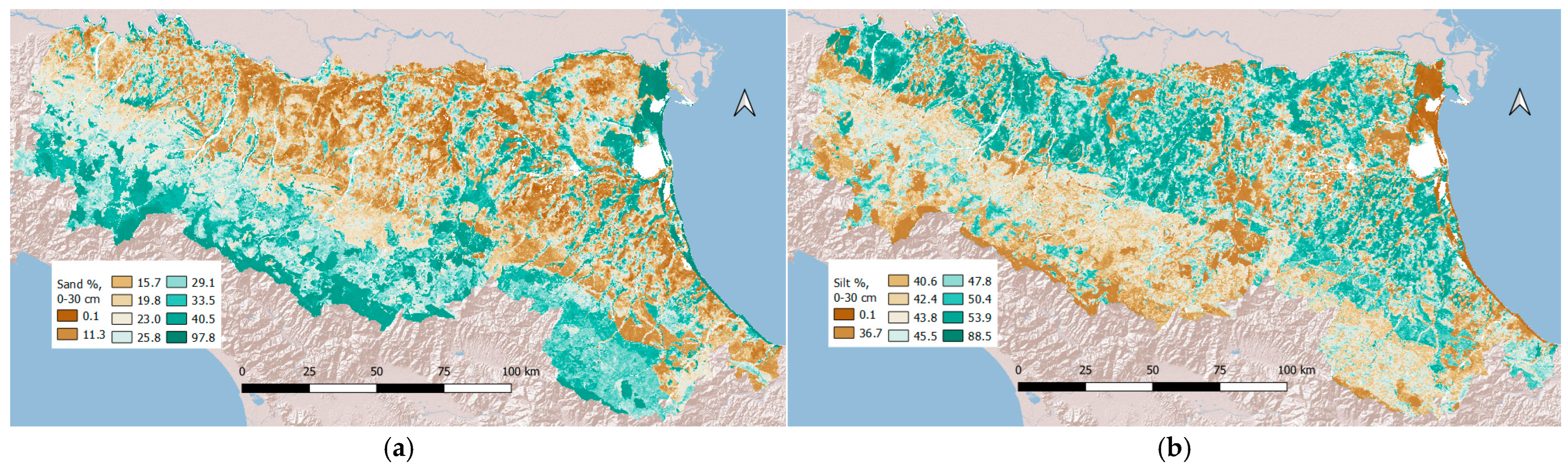
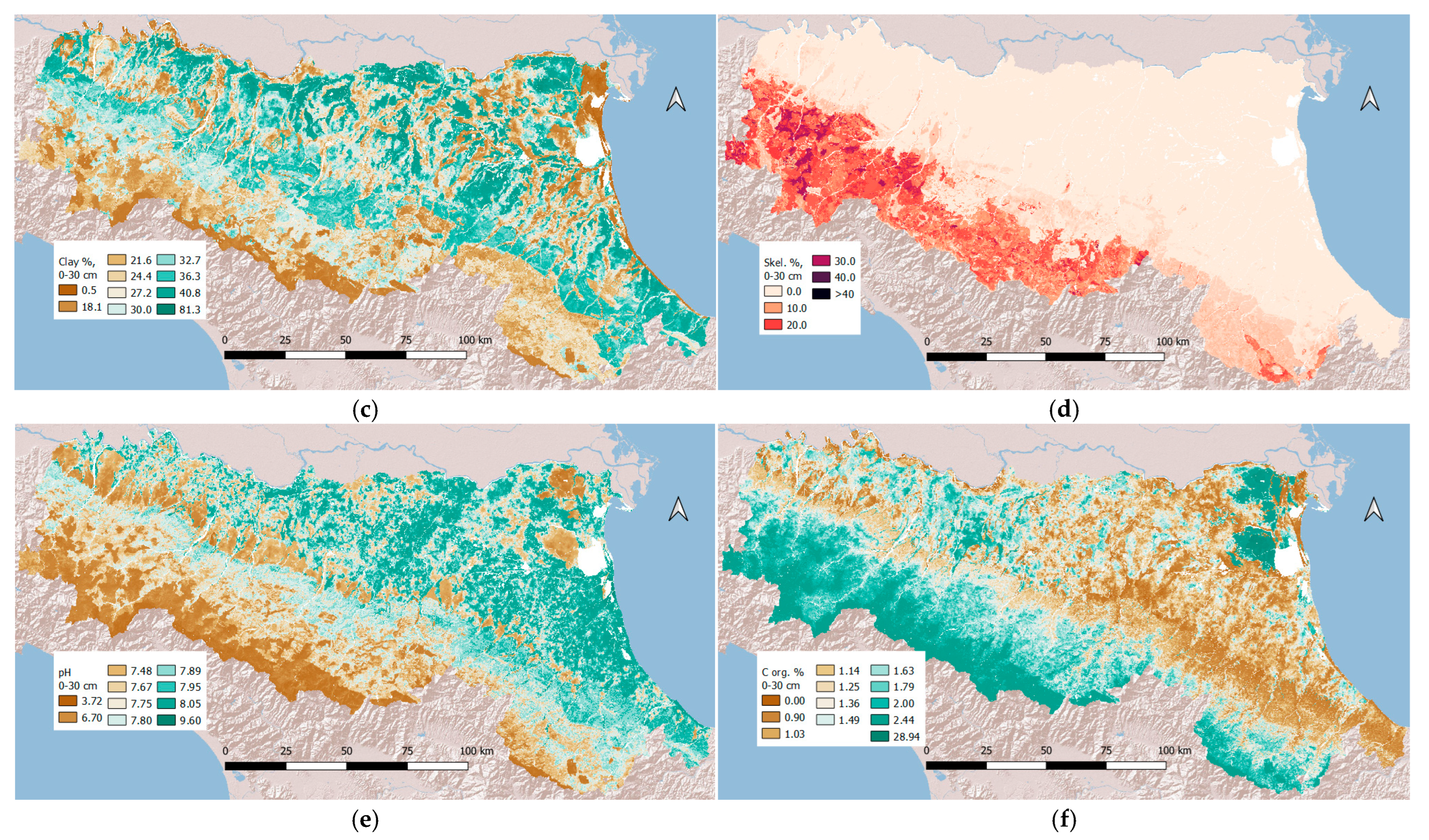
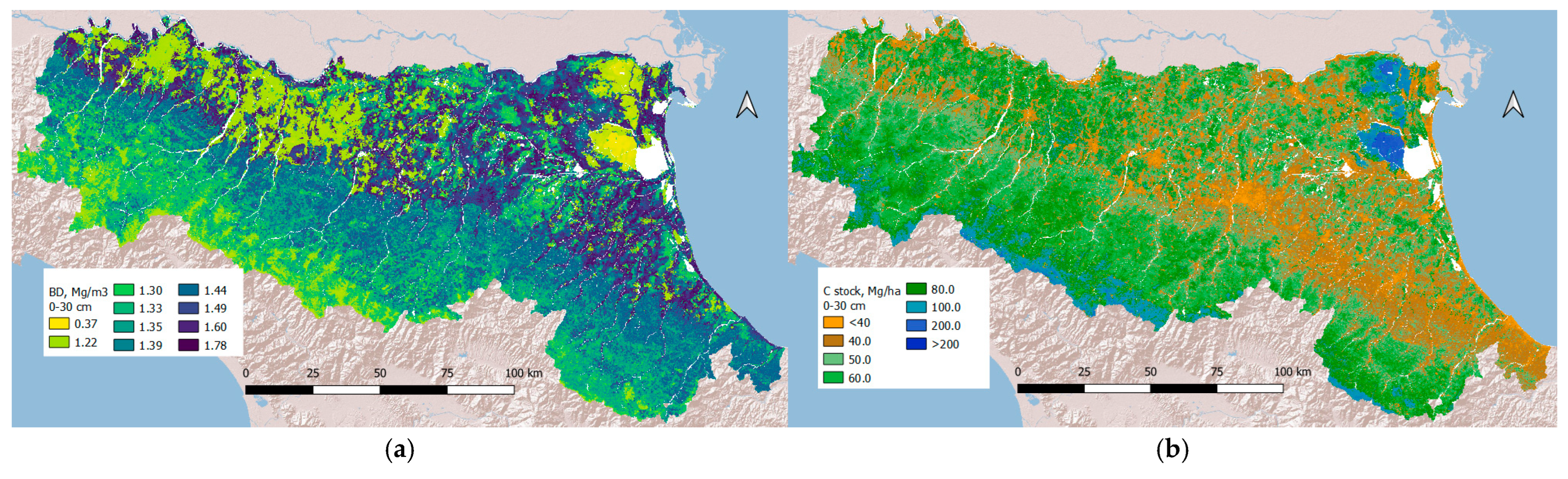
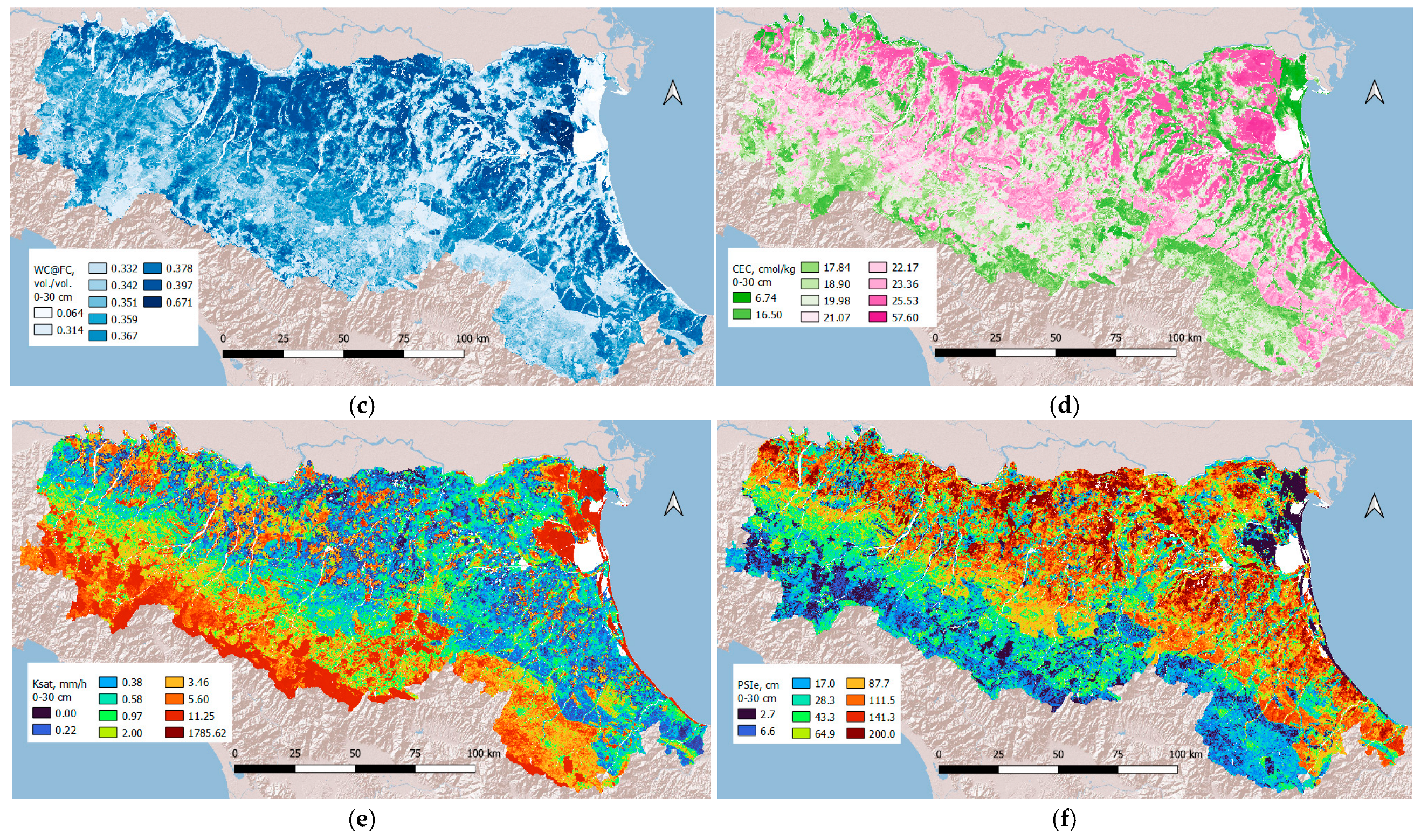
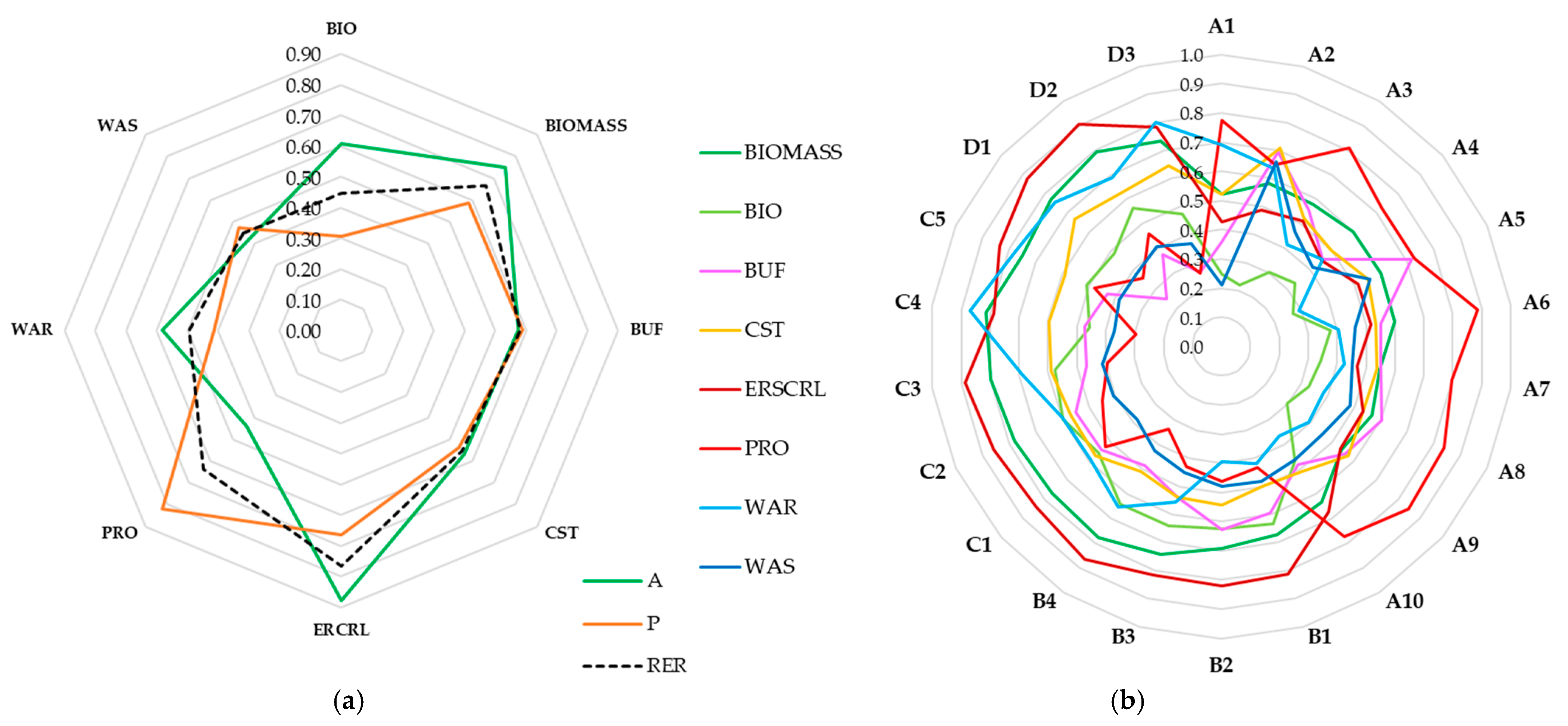
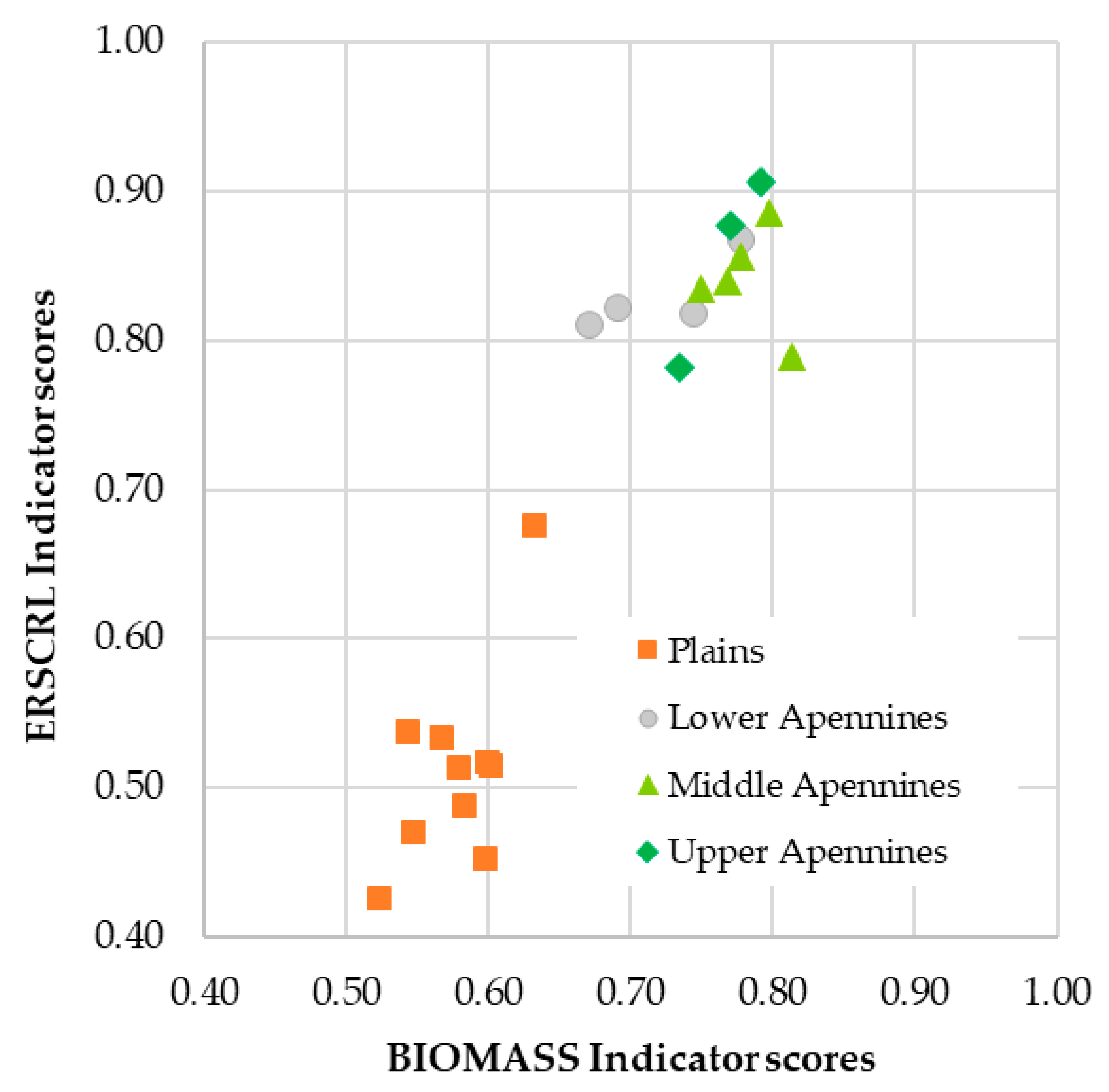
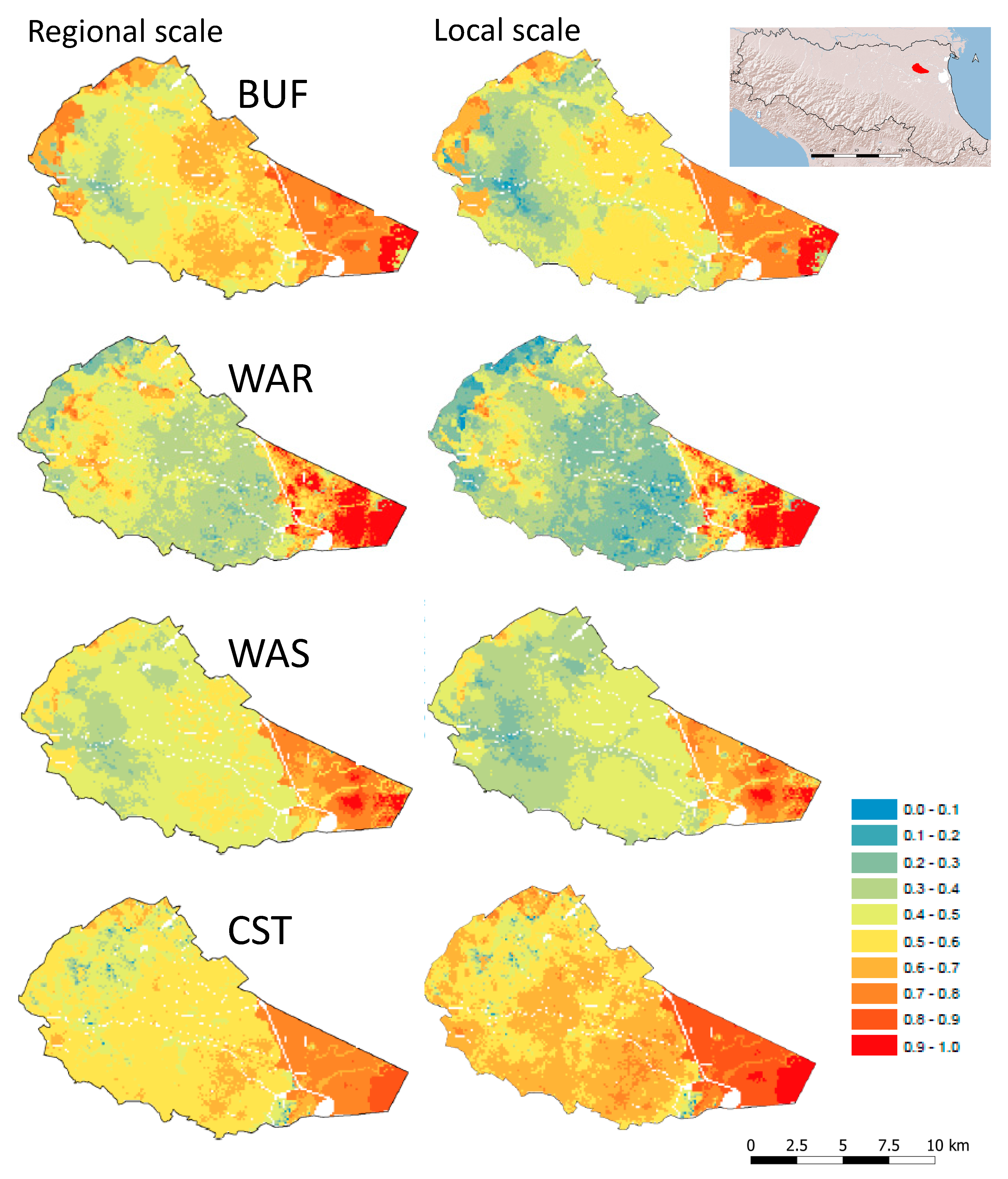

Disclaimer/Publisher’s Note: The statements, opinions and data contained in all publications are solely those of the individual author(s) and contributor(s) and not of MDPI and/or the editor(s). MDPI and/or the editor(s) disclaim responsibility for any injury to people or property resulting from any ideas, methods, instructions or products referred to in the content. |
© 2025 by the authors. Licensee MDPI, Basel, Switzerland. This article is an open access article distributed under the terms and conditions of the Creative Commons Attribution (CC BY) license (https://creativecommons.org/licenses/by/4.0/).