
Geographic Variation in Migratory Grasshopper Recruitment under Projected Climate Change


Abstract
:1. Introduction
2. Materials and Methods
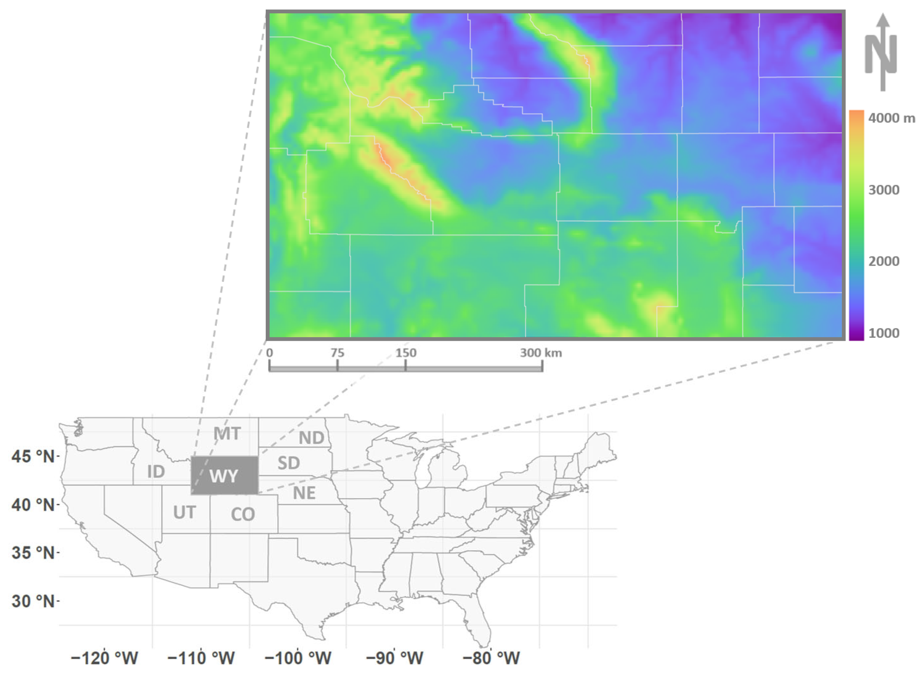
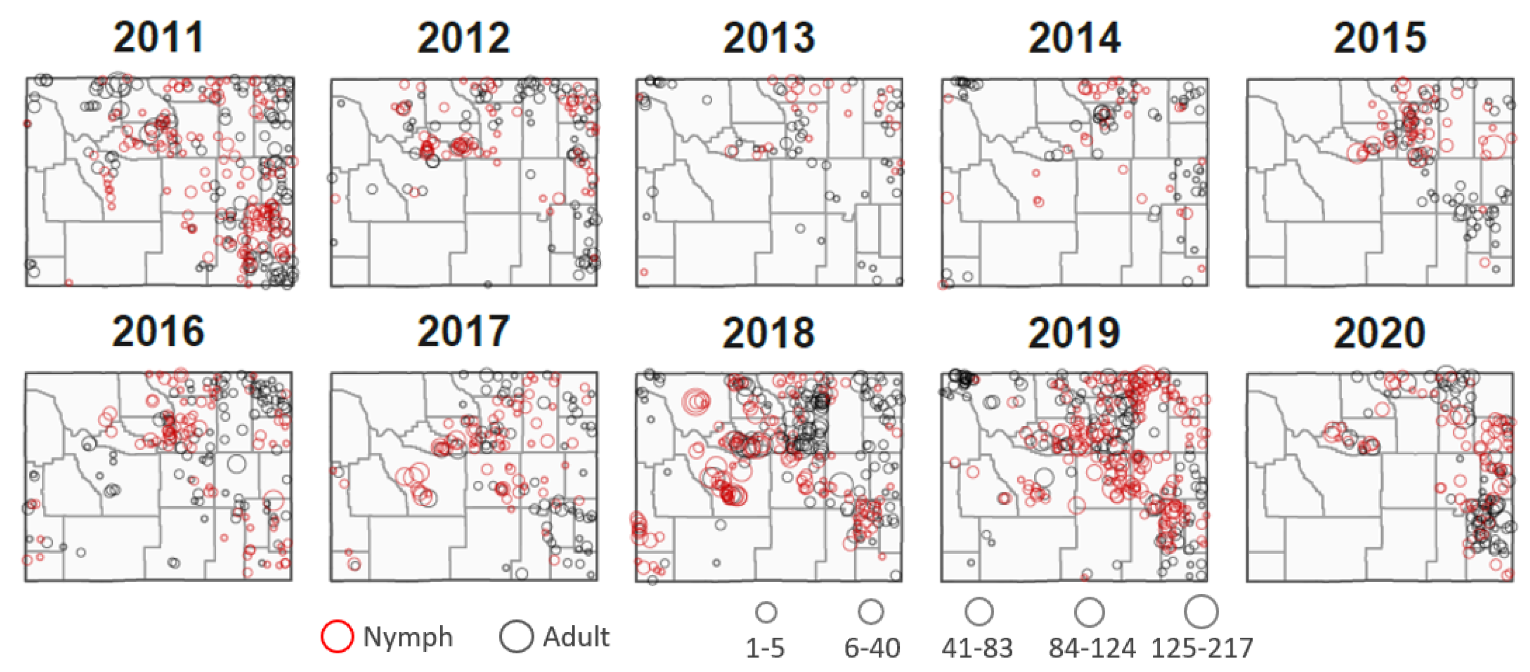
2.1. Study Domain and Observation Data
2.2. Climate and Environmental Data
2.3. Variable Decomposition
2.4. Statistical Model
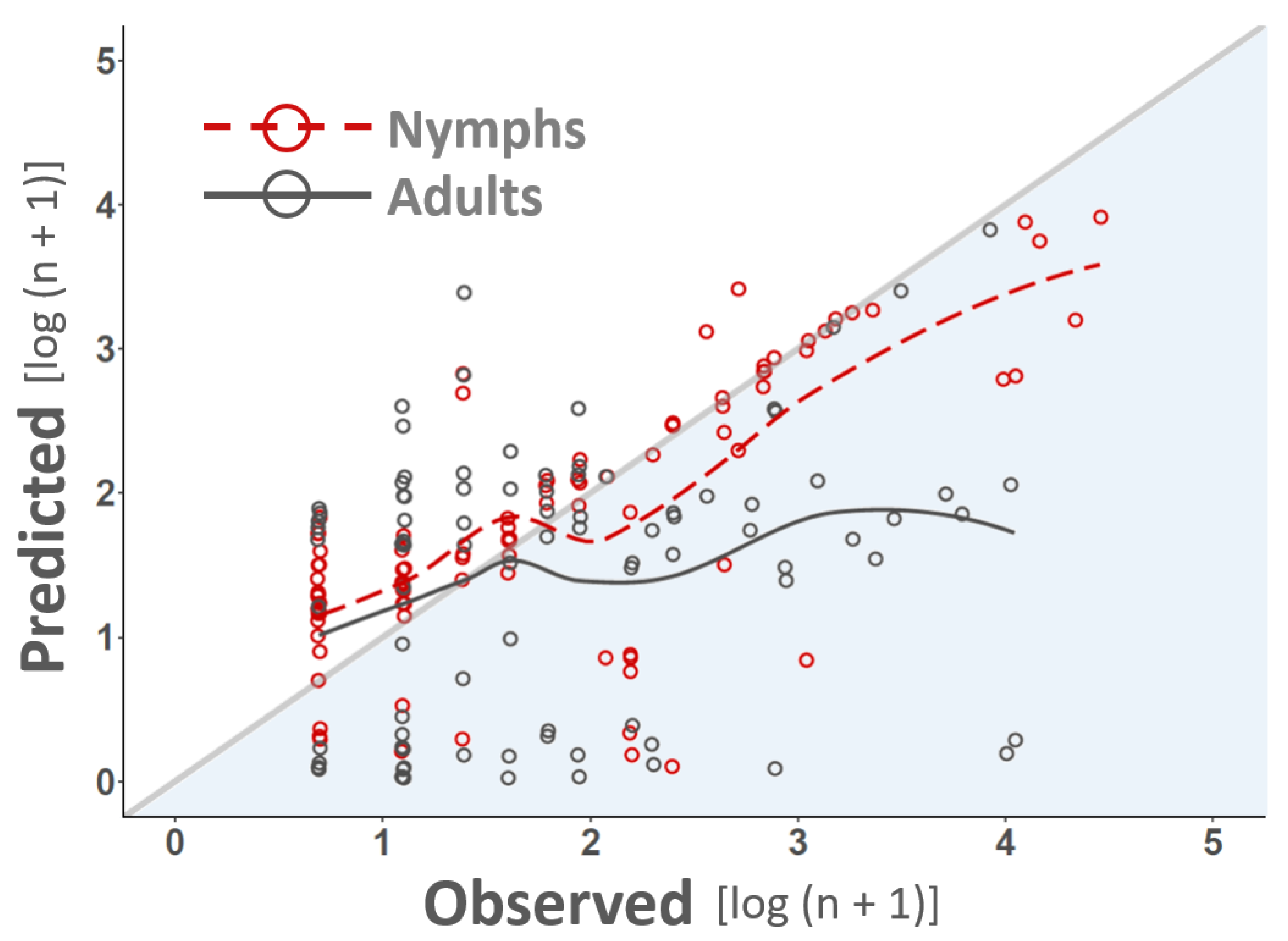
2.5. Model Selection and Validation
2.6. Recruitment Rate Prediction, Consensus, and Forecasts
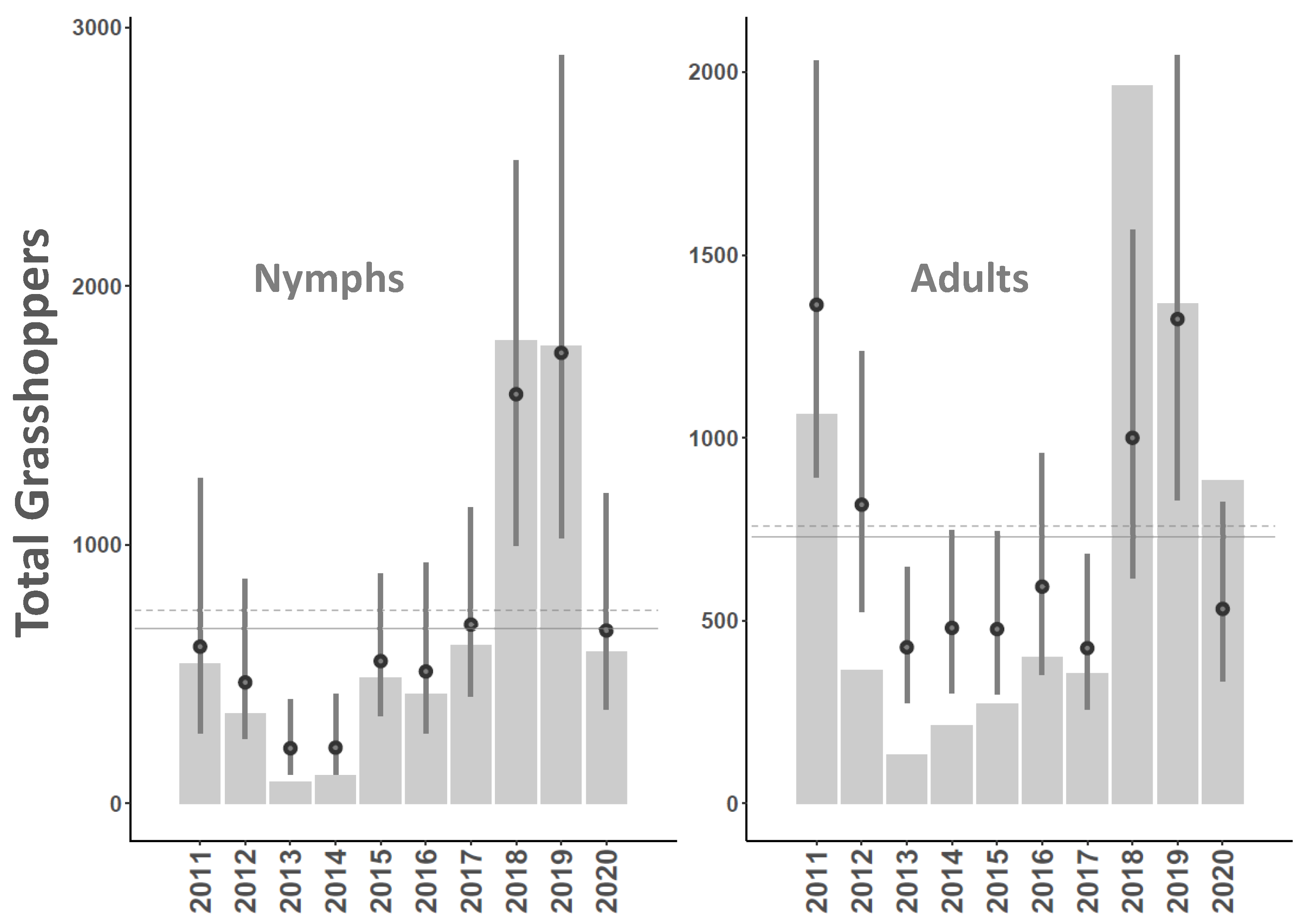
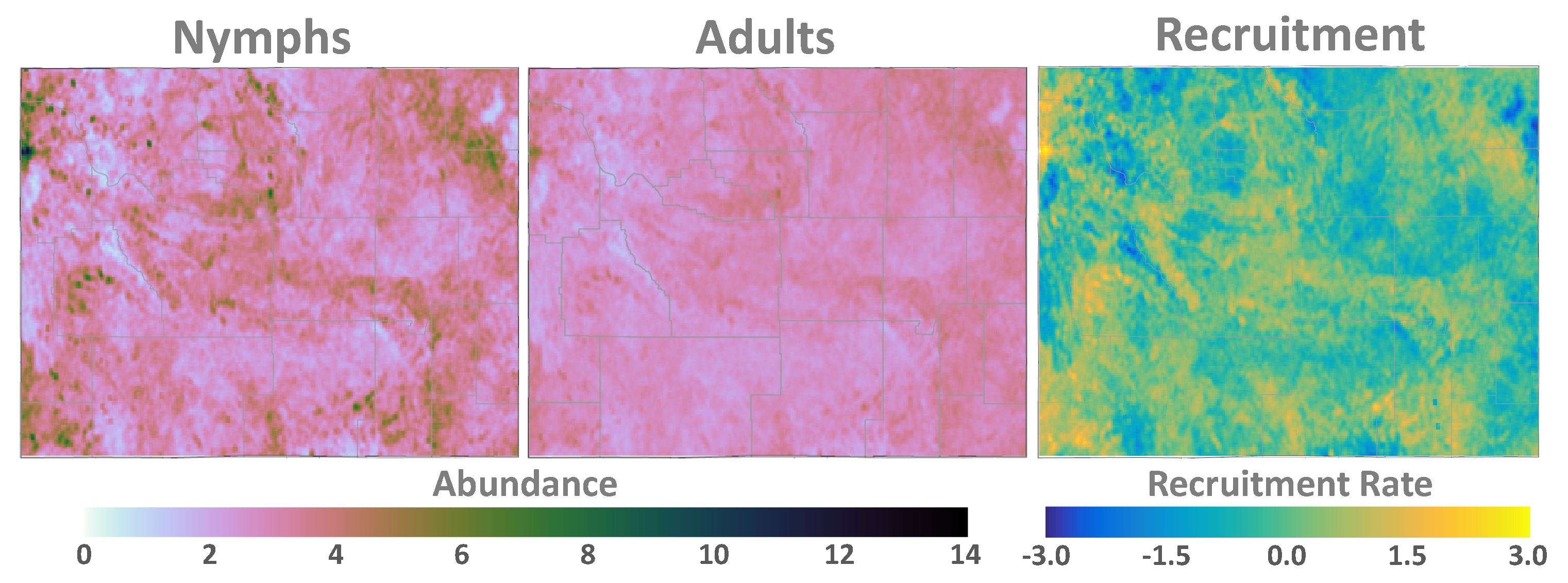
3. Results
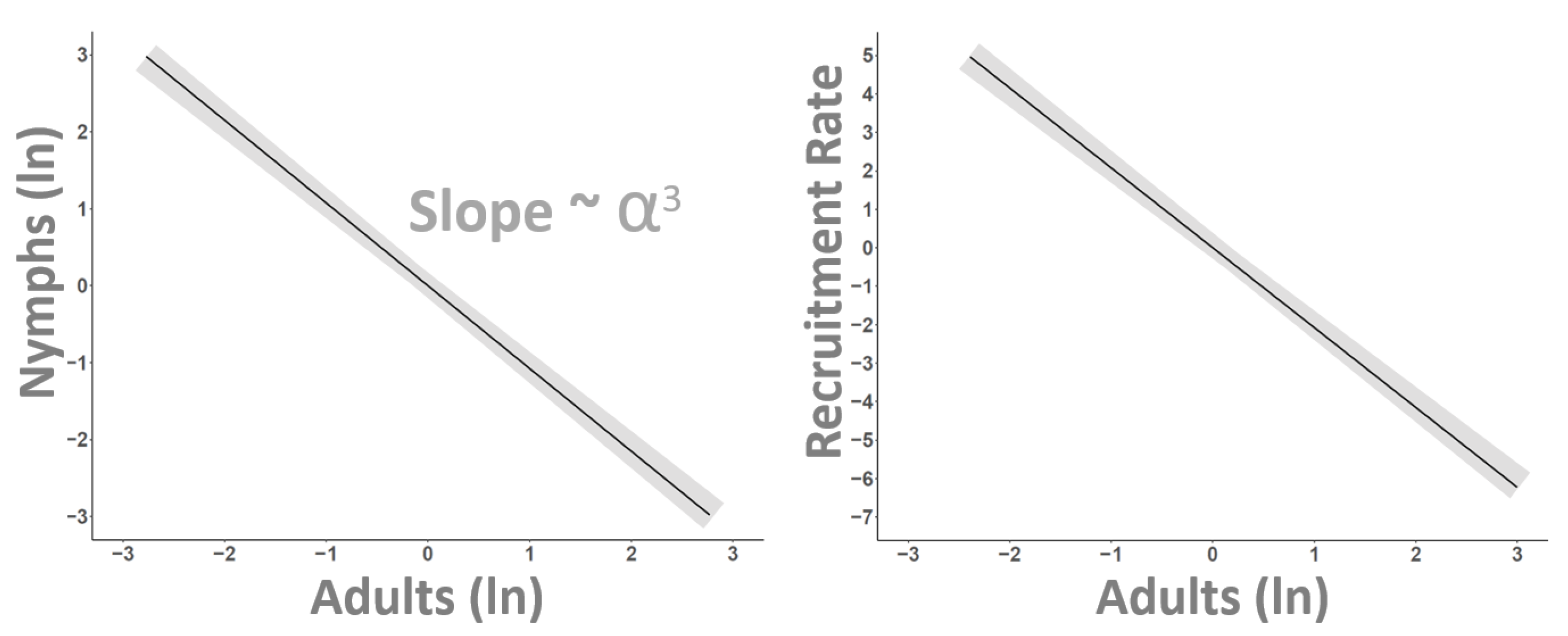
4. Discussion
5. Summary and Conclusions
Supplementary Materials
Author Contributions
Funding
Institutional Review Board Statement
Informed Consent Statement
Data Availability Statement
Acknowledgments
Conflicts of Interest
Abbreviations
| APHIS | Animal and Plant Health Inspection Service |
| ARS | Agricultural Research Service |
| GH | Grasshoppers |
| IPM | Integrated Pest Management |
| PPQ | Plant Protection and Quarantine |
| USDA | United States Department of Agriculture |
References
- Pearson, R.G.; Dawson, T.P. Predicting the impacts of climate change on the distribution of species: Are bioclimate envelope models useful? Glob. Ecol. Biogeogr. 2003, 12, 361–371. [Google Scholar] [CrossRef] [Green Version]
- Humphreys, J.M.; Elsner, J.B.; Jagger, T.H.; Pau, S. A Bayesian geostatistical approach to modeling global distributions of Lygodium microphyllum under projected climate warming. Ecol. Model. 2017, 363, 192–206. [Google Scholar] [CrossRef]
- Capinera, J.L.; Horton, D.R. Geographic Variation in Effects of Weather on Grasshopper Infestation. Environ. Entomol. 1989, 18, 8–14. [Google Scholar] [CrossRef]
- Olfert, O.; Weiss, R.; Turkington, K.; Beckie, H.; Kriticos, D. Bio-climatic approach to assessing the potential impact of climate change on representative crop pests in North America. Clim. Chang. Can. Agric. Environ. Top. Can. Weed Sci. 2012, 8, 45–66. [Google Scholar]
- Jonas, J.L.; Wolesensky, W.; Joern, A. Weather Affects Grasshopper Population Dynamics in Continental Grassland over Annual and Decadal Periods. Rangel. Ecol. Manag. 2015, 68, 29–39. [Google Scholar] [CrossRef]
- Kistner-Thomas, E.; Kumar, S.; Jech, L.; Woller, D.A. Modeling Rangeland Grasshopper (Orthoptera: Acrididae) Population Density Using a Landscape-Level Predictive Mapping Approach. J. Econ. Entomol. 2021, 114, 1557–1567. [Google Scholar] [CrossRef]
- Olfert, O.; Weiss, R.M.; Giffen, D.; Vankosky, M.A. Modeling Ecological Dynamics of a Major Agricultural Pest Insect (Melanoplus sanguinipes; Orthoptera: Acrididae): A Cohort-Based Approach Incorporating the Effects of Weather on Grasshopper Development and Abundance. J. Econ. Entomol. 2020, 114, 122–130. [Google Scholar] [CrossRef]
- Schoof, J.T.; Pryor, S.C.; Surprenant, J. Development of daily precipitation projections for the United States based on probabilistic downscaling. J. Geophys. Res. Atmos. 2010, 115, 1–13. [Google Scholar] [CrossRef]
- Belmecheri, S.; Babst, F.; Hudson, A.R.; Betancourt, J.; Trouet, V. Northern Hemisphere jet stream position indices as diagnostic tools for climate and ecosystem dynamics. Earth Interact. 2017, 21, 1–23. [Google Scholar] [CrossRef]
- Yeh, S.W.; Cai, W.; Min, S.K.; McPhaden, M.J.; Dommenget, D.; Dewitte, B.; Collins, M.; Ashok, K.; An, S.I.; Yim, B.Y.; et al. ENSO Atmospheric Teleconnections and Their Response to Greenhouse Gas Forcing. Rev. Geophys. 2018, 56, 185–206. [Google Scholar] [CrossRef]
- Sun, Q.; Miao, C.; AghaKouchak, A.; Mallakpour, I.; Ji, D.; Duan, Q. Possible Increased Frequency of ENSO-Related Dry and Wet Conditions over Some Major Watersheds in a Warming Climate. Bull. Am. Meteorol. Soc. 2020, 101, E409–E426. [Google Scholar] [CrossRef]
- Reichstein, M.; Bahn, M.; Ciais, P.; Frank, D.; Mahecha, M.D.; Seneviratne, S.I.; Zscheischler, J.; Beer, C.; Buchmann, N.; Frank, D.C.; et al. Climate extremes and the carbon cycle. Nature 2013, 500, 287–295. [Google Scholar] [CrossRef]
- Welti, E.A.; Roeder, K.A.; De Beurs, K.M.; Joern, A.; Kaspari, M. Nutrient dilution and climate cycles underlie declines in a dominant insect herbivore. Proc. Natl. Acad. Sci. USA 2020, 117, 7271–7275. [Google Scholar] [CrossRef] [PubMed]
- Mattson, W.J.; Haack, R.A. The Role of Drought in Outbreaks of Plant-Eating Insects. BioScience 1987, 37, 110–118. [Google Scholar] [CrossRef]
- Parmesan, C.; Root, T.L.; Willig, M.R. Impacts of Extreme Weather and Climate on Terrestrial Biota. Bull. Am. Meteorol. Soc. 2000, 81, 443–450. [Google Scholar] [CrossRef] [Green Version]
- Branson, D.H. Influence of a large late summer precipitation event on food limitation and grasshopper population dynamics in a northern great plains grassland. Environ. Entomol. 2008, 37, 686–695. [Google Scholar] [CrossRef] [Green Version]
- Halsch, C.A.; Shapiro, A.M.; Fordyce, J.A.; Nice, C.C.; Thorne, J.H.; Waetjen, D.P.; Forister, M.L. Insects and recent climate change. Proc. Natl. Acad. Sci. USA 2021, 118, e2002543117. [Google Scholar] [CrossRef]
- Skendžić, S.; Zovko, M.; Živković, I.P.; Lešić, V.; Lemić, D. The Impact of Climate Change on Agricultural Insect Pests. Insects 2021, 12, 440. [Google Scholar] [CrossRef]
- Fartmann, T.; Poniatowski, D.; Holtmann, L. Habitat availability and climate warming drive changes in the distribution of grassland grasshoppers. Agric. Ecosyst. Environ. 2021, 320, 107565. [Google Scholar] [CrossRef]
- Deutsch, C.A.; Tewksbury, J.J.; Tigchelaar, M.; Battisti, D.S.; Merrill, S.C.; Huey, R.B.; Naylor, R.L. Increase in crop losses to insect pests in a warming climate. Science 2018, 361, 916–919. [Google Scholar] [CrossRef] [Green Version]
- Branson, D.H.; Sword, G.A. An experimental analysis of grasshopper community responses to fire and livestock grazing in a northern mixed-grass prairie. Environ. Entomol. 2010, 39, 1441–1446. [Google Scholar] [CrossRef] [PubMed]
- Dakhel, W.H.; Jaronski, S.T.; Schell, S. Control of pest grasshoppers in North America. Insects 2020, 11, 566. [Google Scholar] [CrossRef] [PubMed]
- Belovsky, G.E.; Slade, J.B. Grasshoppers affect grassland ecosystem functioning: Spatial and temporal variation. Basic Appl. Ecol. 2018, 26, 24–34. [Google Scholar] [CrossRef]
- Branson, D.H.; Joern, A.; Sword, G.A. Sustainable Management of Insect Herbivores in Grassland Ecosystems: New Perspectives in Grasshopper Control. BioScience 2006, 56, 743–755. [Google Scholar] [CrossRef]
- Porter, J.; Parry, M.; Carter, T. The potential effects of climatic change on agricultural insect pests. Agric. For. Meteorol. 1991, 57, 221–240. [Google Scholar] [CrossRef]
- Zhang, L.; Lecoq, M.; Latchininsky, A.; Hunter, D. Locust and grasshopper management. Annu. Rev. Entomol. 2019, 64, 15–34. [Google Scholar] [CrossRef]
- Onsager, J.A.; Olfert, O. What Tools have Potential for Grasshopper Pest Management? In Grasshoppers and Grassland Health: Managing Grasshopper Outbreaks without Risking Environmental Disaster; Lockwood, J.A., Latchininsky, A.V., Sergeev, M.G., Eds.; Springer: Dordrecht, The Netherlands, 2000; pp. 145–156. [Google Scholar] [CrossRef]
- Olfert, O.; Weiss, R.M. Impact of grasshopper feeding on selected cultivars of cruciferous oilseed crops. J. Orthoptera Res. 2002, 11, 83–86. [Google Scholar] [CrossRef] [Green Version]
- Carter, M.R.; Macrae, I.V.; Logan, J.A.; Holtzer, T.O. Population Model for Melanoplus sanguinipes (Orthoptera: Acrididae) and an Analysis of Grasshopper Population Fluctuations in Colorado. Environ. Entomol. 1998, 27, 892–901. [Google Scholar] [CrossRef]
- Pfadt, R.E. Field Guide to Common Western Grasshoppers, 3rd ed.; Bulletin 912; Wyoming Agricultural Experiment Station: Laramie, WY, USA, 2002. [Google Scholar]
- Fielding, D.J.; Brusven, M.A. Historical Analysis of Grasshopper (Orthoptera: Acrididae) Population Responses to Climate in Southern Idaho, 1950–1980. Environ. Entomol. 1990, 19, 1786–1791. [Google Scholar] [CrossRef]
- Fielding, D.J. Oviposition Site Selection by the Grasshoppers Melanoplus borealis and M. sanguinipes (Orthoptera: Acrididae). J. Orthoptera Res. 2011, 20, 75–80. [Google Scholar] [CrossRef]
- Hilbert, D.; Logan, J.; Swift, D. A unifying hypothesis of temperature effects on egg development and diapause of the migratory grasshopper, Melanoplus sanguinipes (Orthoptera: Acrididae). J. Theor. Biol. 1985, 112, 827–838. [Google Scholar] [CrossRef]
- Hewitt, G.B. Hatching and Development of Rangeland Grasshoppers 1 in Relation to Forage Growth, Temperature, and Precipitation. Environ. Entomol. 1979, 8, 24–29. [Google Scholar] [CrossRef]
- Lactin, D.J.; Johnson, D.L. Temperature-Dependent Feeding Rates of Melanoplus sanguinipes Nymphs (Orthoptera: Acrididae) Laboratory Trials. Environ. Entomol. 1995, 24, 1291–1296. [Google Scholar] [CrossRef]
- Lactin, D.J.; Johnson, D.L. Behavioural optimization of body temperature by nymphal grasshoppers (Melanoplus sanguinipes, Orthoptera: Acrididae) in temperature gradients established using incandescent bulbs. J. Therm. Biol. 1996, 21, 231–238. [Google Scholar] [CrossRef]
- University of Wyoming. Fact Sheet: Migratory Grasshopper, Melanoplus sanguinipes (Fabricius). 2021. Available online: http://www.uwyo.edu/entomology/grasshoppers/field-guide/mesa.html (accessed on 2 December 2021).
- Kemp, W.P. Temporal variation in rangeland grasshopper (Orthoptera: Acrididae) communities in the steppe region of Montana, USA. Can. Entomol. 1992, 124, 437–450. [Google Scholar] [CrossRef]
- Gaillard, J.; Coulson, T.; Festa-Bianchet, M. Recruitment. In Encyclopedia of Ecology; Jørgensen, S.E., Fath, B.D., Eds.; Academic Press: Oxford, UK, 2008; pp. 2982–2986. [Google Scholar] [CrossRef]
- Olson, D.M.; Dinerstein, E. The Global 200: Priority Ecoregions for Global Conservation. Ann. Mo. Bot. Gard. 2002, 89, 199–224. [Google Scholar] [CrossRef]
- Buisson, L.; Thuiller, W.; Casajus, N.; Lek, S.; Grenouillet, G. Uncertainty in ensemble forecasting of species distribution. Glob. Chang. Biol. 2010, 16, 1145–1157. [Google Scholar] [CrossRef]
- Thuiller, W. Patterns and uncertainties of species’ range shifts under climate change. Glob. Chang. Biol. 2004, 10, 2020–2027. [Google Scholar] [CrossRef]
- Marmion, M.; Parviainen, M.; Luoto, M.; Heikkinen, R.K.; Thuiller, W. Evaluation of consensus methods in predictive species distribution modelling. Divers. Distrib. 2009, 15, 59–69. [Google Scholar] [CrossRef]
- Eyring, V.; Bony, S.; Meehl, G.A.; Senior, C.A.; Stevens, B.; Stouffer, R.J.; Taylor, K.E. Overview of the Coupled Model Intercomparison Project Phase 6 (CMIP6) experimental design and organization. Geosci. Model Dev. 2016, 9, 1937–1958. [Google Scholar] [CrossRef] [Green Version]
- Sanderson, B.M.; Knutti, R.; Caldwell, P. A Representative Democracy to Reduce Interdependency in a Multimodel Ensemble. J. Clim. 2015, 28, 5171–5194. [Google Scholar] [CrossRef] [Green Version]
- Sanderson, B.M.; Knutti, R.; Caldwell, P. Addressing Interdependency in a Multimodel Ensemble by Interpolation of Model Properties. J. Clim. 2015, 28, 5150–5170. [Google Scholar] [CrossRef]
- Boucher, O.; Denvil, S.; Levavasseur, G.; Cozic, A.; Caubel, A.; Foujols, M.A.; Meurdesoif, Y.; Balkanski, Y.; Checa-Garcia, R.; Hauglustaine, D.; et al. IPSL IPSL-CM6A-LR-INCA Model output Prepared for CMIP6 AerChemMIP. 2020. Available online: https://doi.org/10.22033/ESGF/CMIP6.13581 (accessed on 2 December 2021).
- Swart, N.C.; Cole, J.N.; Kharin, V.V.; Lazare, M.; Scinocca, J.F.; Gillett, N.P.; Anstey, J.; Arora, V.; Christian, J.R.; Jiao, Y.; et al. CCCma CanESM5 Model Output Prepared for CMIP6 C4MIP. 2019. Available online: https://doi.org/10.22033/ESGF/CMIP6.1301 (accessed on 2 December 2021).
- Takemura, T. MIROC MIROC6 Model Output Prepared for CMIP6 AerChemMIP. 2019. Available online: https://doi.org/10.22033/ESGF/CMIP6.9121 (accessed on 2 December 2021).
- Fick, S.E.; Hijmans, R.J. WorldClim 2: New 1-km spatial resolution climate surfaces for global land areas. Int. J. Climatol. 2017, 37, 4302–4315. [Google Scholar] [CrossRef]
- Riahi, K.; van Vuuren, D.P.; Kriegler, E.; Edmonds, J.; O’Neill, B.C.; Fujimori, S.; Bauer, N.; Calvin, K.; Dellink, R.; Fricko, O.; et al. The Shared Socioeconomic Pathways and their energy, land use, and greenhouse gas emissions implications: An overview. Glob. Environ. Chang. 2017, 42, 153–168. [Google Scholar] [CrossRef] [Green Version]
- Poggio, L.; de Sousa, L.M.; Batjes, N.H.; Heuvelink, G.B.M.; Kempen, B.; Ribeiro, E.; Rossiter, D. SoilGrids 2.0: Producing soil information for the globe with quantified spatial uncertainty. SOIL 2021, 7, 217–240. [Google Scholar] [CrossRef]
- Tuanmu, M.N.; Jetz, W. A global, remote sensing-based characterization of terrestrial habitat heterogeneity for biodiversity and ecosystem modelling. Glob. Ecol. Biogeogr. 2015, 24, 1329–1339. [Google Scholar] [CrossRef]
- Austin, M. Spatial prediction of species distribution: An interface between ecological theory and statistical modelling. Ecol. Model. 2002, 157, 101–118. [Google Scholar] [CrossRef] [Green Version]
- De Marco, J.P.; Nóbrega, C.C. Evaluating collinearity effects on species distribution models: An approach based on virtual species simulation. PLoS ONE 2018, 13, e0202403. [Google Scholar] [CrossRef]
- Dormann, C.F.; Purschke, O.; Márquez, J.R.G.; Lautenbach, S.; Schröder, B. Components of uncertainty in species distribution analysis: A case study of the great grey shrike. Ecology 2008, 89, 3371–3386. [Google Scholar] [CrossRef]
- Dupin, M.; Reynaud, P.; Jarošík, V.; Baker, R.; Brunel, S.; Eyre, D.; Pergl, J.; Makowski, D. Effects of the Training Dataset Characteristics on the Performance of Nine Species Distribution Models: Application to Diabrotica virgifera virgifera. PLoS ONE 2011, 6, e20957. [Google Scholar] [CrossRef]
- Silva, D.P.; Gonzalez, V.H.; Melo, G.A.; Lucia, M.; Alvarez, L.J.; De Marco, P. Seeking the flowers for the bees: Integrating biotic interactions into niche models to assess the distribution of the exotic bee species Lithurgus huberi in South America. Ecol. Model. 2014, 273, 200–209. [Google Scholar] [CrossRef]
- Cruz-Cárdenas, G.; López-Mata, L.; Villaseñor, J.L.; Ortiz, E. Potential species distribution modeling and the use of principal component analysis as predictor variables. Rev. Mex. De Biodivers. 2014, 85, 189–199. [Google Scholar] [CrossRef]
- Velazco, S.J.E.; Galvão, F.; Villalobos, F.; De Marco Júnior, P. Using worldwide edaphic data to model plant species niches: An assessment at a continental extent. PLoS ONE 2017, 12, e0186025. [Google Scholar] [CrossRef] [PubMed] [Green Version]
- Jombart, T.; Devillard, S.; Balloux, F.; Falush, D. Discriminant analysis of principal components: A new method for the analysis of genetically structured populations. BMC Genet. 2010, 11, 94. [Google Scholar] [CrossRef] [Green Version]
- Palinski, R.; Pauszek, S.J.; Humphreys, J.M.; Peters, D.P.; McVey, D.S.; Pelzel-McCluskey, A.M.; Derner, J.D.; Burruss, N.D.; Arzt, J.; Rodriguez, L.L. Evolution and expansion dynamics of a vector-borne virus: 2004–2006 vesicular stomatitis outbreak in the western USA. Ecosphere 2021, 12, e03793. [Google Scholar] [CrossRef]
- Jombart, T.; Ahmed, I. Adegenet 1.3-1: New tools for the analysis of genome-wide SNP data. Bioinformatics 2011, 27, 3070–3071. [Google Scholar] [CrossRef] [Green Version]
- Diggle, P.J.; Menezes, R.; Su, T.l. Geostatistical inference under preferential sampling. J. R. Stat. Soc. Ser. C (Appl. Stat.) 2010, 59, 191–232. [Google Scholar] [CrossRef]
- Pennino, M.G.; Paradinas, I.; Illian, J.B.; Muñoz, F.; Bellido, J.M.; López-Quílez, A.; Conesa, D. Accounting for preferential sampling in species distribution models. Ecol. Evol. 2019, 9, 653–663. [Google Scholar] [CrossRef]
- Stenkamp-Strahm, C.; Patyk, K.; McCool-Eye, M.J.; Fox, A.; Humphreys, J.; James, A.; South, D.; Magzamen, S. Using geospatial methods to measure the risk of environmental persistence of avian influenza virus in South Carolina. Spat. Spatio-Temporal Epidemiol. 2020, 34, 100342. [Google Scholar] [CrossRef]
- Lindgren, F.; Rue, H.; Lindström, J. An explicit link between Gaussian fields and Gaussian Markov random field: The stochastic partial differential equations approach. J. R. Stat. Soc. Ser. B Stat. Methodol. 2011, 73, 423–498. [Google Scholar] [CrossRef] [Green Version]
- Simpson, D.; Illian, J.B.; Lindgren, F.; Sørbye, S.H.; Rue, H. Going off grid: Computationally efficient inference for log-Gaussian Cox processes. Biometrika 2016, 103, 49–70. [Google Scholar] [CrossRef] [Green Version]
- Krainski, E.; Gómez Rubio, V.; Bakka, H.; Lenzi, A.; Castro-Camilo, D.; Simpson, D.; Lindgren, F.; Rue, H. Advanced Spatial Modeling with Stochastic Partial Differential Equations Using R and INLA; Chapman and Hall/CRC: Boca Raton, FL, USA, 2018. [Google Scholar] [CrossRef]
- Humphreys, J.M.; Murrow, J.L.; Sullivan, J.D.; Prosser, D.J. Seasonal occurrence and abundance of dabbling ducks across the continental United States: Joint spatio-temporal modelling for the Genus Anas. Divers. Distrib. 2019, 25, 1497–1508. [Google Scholar] [CrossRef] [Green Version]
- Humphreys, J.M.; Mahjoor, A.; Reiss, C.K.; Uribe, A.A.; Brown, M.T. A geostatistical model for estimating edge effects and cumulative human disturbance in wetlands and coastal waters. Int. J. Geogr. Inf. Syst. 2020, 34, 1508–1529. [Google Scholar] [CrossRef]
- Humphreys, J.M.; Ramey, A.M.; Douglas, D.C.; Mullinax, J.M.; Soos, C.; Link, P.; Walther, P.; Prosser, D.J. Waterfowl occurrence and residence time as indicators of H5 and H7 avian influenza in North American Poultry. Sci. Rep. 2020, 10, 2592. [Google Scholar] [CrossRef] [PubMed]
- Sultaire, S.M.; Humphreys, J.M.; Zuckerberg, B.; Pauli, J.N.; Roloff, G.J. Spatial variation in bioclimatic relationships for a snow-adapted species along a discontinuous southern range boundary. J. Biogeogr. 2022, 49, 66–78. [Google Scholar] [CrossRef]
- Humphreys, J.M.; Douglas, D.C.; Ramey, A.M.; Mullinax, J.M.; Soos, C.; Link, P.; Walther, P.; Prosser, D.J. The spatial–temporal relationship of blue-winged teal to domestic poultry: Movement state modelling of a highly mobile avian influenza host. J. Appl. Ecol. 2021, 58, 2040–2052. [Google Scholar] [CrossRef]
- Kemp, W.P.; Dennis, B. Density dependence in rangeland grasshoppers (Orthoptera: Acrididae). Oecologia 1993, 96, 1–8. [Google Scholar] [CrossRef]
- Rue, H.; Martino, S.; Chopin, N. Approximate Bayesian inference for latent Gaussian models by using integrated nested Laplace approximations. J. R. Stat. Soc. Ser. B Stat. Methodol. 2009, 71, 319–392. [Google Scholar] [CrossRef]
- Martins, T.G.; Simpson, D.; Lindgren, F.; Rue, H. Bayesian computing with INLA: New features. Comput. Stat. Data Anal. 2013, 67, 68–83. [Google Scholar] [CrossRef] [Green Version]
- Lindgren, F.; Rue, H. Bayesian Spatial Modelling with R-INLA. J. Stat. Softw. 2015, 63, 1–25. [Google Scholar] [CrossRef] [Green Version]
- Verbosio, F.; De Coninck, A.; Kourounis, D.; Schenk, O. Enhancing the scalability of selected inversion factorization algorithms in genomic prediction. J. Comput. Sci. 2017, 22, 99–108. [Google Scholar] [CrossRef]
- Kourounis, D.; Fuchs, A.; Schenk, O. Towards the Next Generation of Multiperiod Optimal Power Flow Solvers. IEEE Trans. Power Syst. 2018, 33, 4005–4014. [Google Scholar] [CrossRef]
- van Niekerk, J.; Bakka, H.; Rue, H.; Schenk, O. New frontiers in Bayesian modeling using the INLA package in R. arXiv 2021, arXiv:1907.10426. [Google Scholar] [CrossRef]
- Simpson, D.; Rue, H.; Riebler, A.; Martins, T.G.; Sørbye, S.H. Penalising Model Component Complexity: A Principled, Practical Approach to Constructing Priors. Stat. Sci. 2017, 32, 1–28. [Google Scholar] [CrossRef]
- Riebler, A.; Sørbye, S.H.; Simpson, D.; Rue, H.; Lawson, A.B.; Lee, D.; MacNab, Y. An intuitive Bayesian spatial model for disease mapping that accounts for scaling. Stat. Methods Med. Res. 2016, 25, 1145–1165. [Google Scholar] [CrossRef] [Green Version]
- Gelman, A.; Hwang, J.; Vehtari, A. Understanding predictive information criteria for Bayesian models. Stat. Comput. 2014, 24, 997–1016. [Google Scholar] [CrossRef]
- Gneiting, T.; Raftery, A.E. Strictly Proper Scoring Rules, Prediction, and Estimation. J. Am. Stat. Assoc. 2007, 102, 359–378. [Google Scholar] [CrossRef]
- Hooten, M.B.; Hobbs, N.T. A guide to Bayesian model selection for ecologists. Ecol. Monogr. 2015, 85, 3–28. [Google Scholar] [CrossRef]
- Berryman, A.A. Principles of Population Dynamics and Their Application; Garland Science: New York, NY, USA, 2020. [Google Scholar]
- Turchin, P. Complex Population Dynamics: A Theoretical/Empirical Synthesis; Princeton University Press: Princeton, NJ, USA, 2013. [Google Scholar] [CrossRef]
- Hoeting, J.A.; Madigan, D.; Raftery, A.E.; Volinsky, C.T. Bayesian Model Averaging: A Tutorial. Stat. Sci. 1999, 14, 382–401. [Google Scholar]
- Gómez-Rubio, V.; Bivand, R.S.; Rue, H. Bayesian Model Averaging with the Integrated Nested Laplace Approximation. Econometrics 2020, 8, 23. [Google Scholar] [CrossRef]
- WRB, I.W.G. International soil classification system for naming soils and creating legends for soil maps. World Ref. Base Soil Resources 2014 (Update 2015) 2015, 106, 1–203. [Google Scholar]
- Dingle, H.; Mousseau, T.A.; Scott, S.M. Altitudinal variation in life cycle syndromes of California populations of the grasshopper, Melanoplus sanguinipes (F.). Oecologia 1990, 84, 199–206. [Google Scholar] [CrossRef] [PubMed]
- Parmesan, C. Ecological and Evolutionary Responses to Recent Climate Change. Annu. Rev. Ecol. Evol. Syst. 2006, 37, 637–669. [Google Scholar] [CrossRef] [Green Version]
- Bässler, C.; Hothorn, T.; Brandl, R.; Müller, J. Insects Overshoot the Expected Upslope Shift Caused by Climate Warming. PLoS ONE 2013, 8, e65842. [Google Scholar] [CrossRef] [Green Version]
- Prinster, A.J.; Resasco, J.; Nufio, C.R. Weather variation affects the dispersal of grasshoppers beyond their elevational ranges. Ecol. Evol. 2020, 10, 14411–14422. [Google Scholar] [CrossRef] [PubMed]
- Srygley, R.B.; Jaronski, S.T. Increasing temperature reduces cuticular melanism and immunity to fungal infection in a migratory insect. Ecol. Entomol. 2022, 47, 109–113. [Google Scholar] [CrossRef]
- Pfadt, R.E. Species Richness, Density, And Diversity Of Grasshoppers (Orthoptera: Acrididae) in a Habitat of the Mixed Grass Prairie. Can. Entomol. 1984, 116, 703–709. [Google Scholar] [CrossRef]
- Fielding, D.J.; Brusven, M.A. Food and Habitat Preferences of Melanoplus sanguinipes and Aulocara elliotti (Orthoptera: Acrididae) on Disturbed Rangeland in Southern Idaho. J. Econ. Entomol. 1992, 85, 783–788. [Google Scholar] [CrossRef]
- Porter, E.E.; Redak, R.A.; Braker, H.E. Density, Biomass, and Diversity of Grasshoppers (Orthoptera: Acrididae) in a California Native Grassland. Great Basin Nat. 1996, 56, 172–176. [Google Scholar]
- Branson, D.H. Relationships between plant diversity and grasshopper diversity and abundance in the Little Missouri National Grassland. Psyche 2011, 2011, 1–7. [Google Scholar] [CrossRef]
- Merow, C.; Bois, S.T.; Allen, J.M.; Xie, Y.; Silander, J.A. Climate change both facilitates and inhibits invasive plant ranges in New England. Proc. Natl. Acad. Sci. USA 2017, 114, E3276–E3284. [Google Scholar] [CrossRef] [PubMed] [Green Version]
- Briscoe, N.J.; Elith, J.; Salguero-Gómez, R.; Lahoz-Monfort, J.J.; Camac, J.S.; Giljohann, K.M.; Holden, M.H.; Hradsky, B.A.; Kearney, M.R.; McMahon, S.M.; et al. Forecasting species range dynamics with process-explicit models: Matching methods to applications. Ecol. Lett. 2019, 22, 1940–1956. [Google Scholar] [CrossRef] [PubMed] [Green Version]
- Branson, D.H. Reproduction and survival in Melanoplus sanguinipes (Orthoptera: Acrididae) in response to resource availability and population density: The role of exploitative competition. Can. Entomol. 2003, 135, 415–426. [Google Scholar] [CrossRef]
- Branson, D.H. Relative importance of nymphal and adult resource availability for reproductive allocation in Melanoplus sanguinipes (Orthoptera: Acrididae). J. Orthoptera Res. 2004, 13, 239–245. [Google Scholar] [CrossRef] [Green Version]
- Haig, D. From Darwin to Derrida: Selfish Genes, Social Selves, and the Meanings of Life; MIT Press: Cambridge, MA, USA, 2020. [Google Scholar]
- Ullman, E.L. Human Geography and area Research. Ann. Assoc. Am. Geogr. 1953, 43, 54–66. [Google Scholar] [CrossRef]
- Shen, X.; Liu, B.; Jiang, M.; Lu, X. Marshland Loss Warms Local Land Surface Temperature in China. Geophys. Res. Lett. 2020, 47, e2020GL087648. [Google Scholar] [CrossRef] [Green Version]
- Shen, X.; Jiang, M.; Lu, X.; Liu, X.; Liu, B.; Zhang, J.; Wang, X.; Tong, S.; Lei, G.; Wang, S.; et al. Aboveground biomass and its spatial distribution pattern of herbaceous marsh vegetation in China. Sci. China Earth Sci. 2021, 64, 1115–1125. [Google Scholar] [CrossRef]


| Model | DIC | WAIC | lCPO | Stage |
|---|---|---|---|---|
| Model1 | 10,322 | 15,271 | 1.28 | Adult (I) |
| Model2 | 9905 | 15,757 | 1.20 | Nymph (I) |
| Model3 | 10,134 | 14,977 | 1.13 | Adult (J) |
| 9487 | 11,467 | 1.08 | Nymph (J) |
| Hyperparameter | Mean | sd | 2.5 Q | 97.5 Q |
|---|---|---|---|---|
| Spatial Range | 16.02 | 0.44 | 15.18 | 16.90 |
| Stdev | 0.43 | 0.01 | 0.41 | 0.44 |
| Group | 0.98 | <0.01 | 0.98 | 0.98 |
| Spatial Range | 17.67 | 0.57 | 16.58 | 18.83 |
| Stdev | 0.53 | 0.01 | 0.51 | 0.55 |
| Group | 0.99 | <0.01 | 0.99 | 0.99 |
| (adults) | 6.06 | 0.05 | 5.98 | 6.17 |
| (nymphs) | 10.39 | 0.19 | 10.12 | 10.83 |
| (adults-nymphs) | −1.07 | 0.03 | −1.14 | −1.03 |
Publisher’s Note: MDPI stays neutral with regard to jurisdictional claims in published maps and institutional affiliations. |
© 2022 by the authors. Licensee MDPI, Basel, Switzerland. This article is an open access article distributed under the terms and conditions of the Creative Commons Attribution (CC BY) license (https://creativecommons.org/licenses/by/4.0/).
Share and Cite
Humphreys, J.M.; Srygley, R.B.; Branson, D.H. Geographic Variation in Migratory Grasshopper Recruitment under Projected Climate Change. Geographies 2022, 2, 12-30. https://doi.org/10.3390/geographies2010003
Humphreys JM, Srygley RB, Branson DH. Geographic Variation in Migratory Grasshopper Recruitment under Projected Climate Change. Geographies. 2022; 2(1):12-30. https://doi.org/10.3390/geographies2010003
Chicago/Turabian StyleHumphreys, John M., Robert B. Srygley, and David H. Branson. 2022. "Geographic Variation in Migratory Grasshopper Recruitment under Projected Climate Change" Geographies 2, no. 1: 12-30. https://doi.org/10.3390/geographies2010003
APA StyleHumphreys, J. M., Srygley, R. B., & Branson, D. H. (2022). Geographic Variation in Migratory Grasshopper Recruitment under Projected Climate Change. Geographies, 2(1), 12-30. https://doi.org/10.3390/geographies2010003