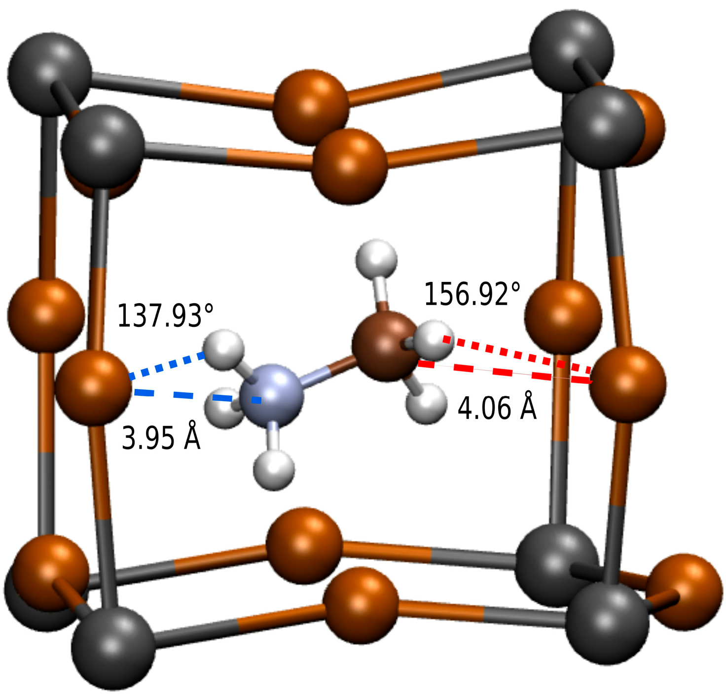
Correlation Between C–H∙∙∙Br and N–H∙∙∙Br Hydrogen Bond Formation in Perovskite CH₃NH₃PbBr₃: A Study Based on Statistical Analysis

Abstract

This study investigates the potential correlation between C—H···Br and N—H···Br hydrogen bonds in CH₃NH₃PbBr₃ over a broad temperature range (50–350 K), using a statistical analysis of molecular dynamics simulations. The analysis focused on quantifying the relationship between both hydrogen bond types via Pearson and Spearman correlation coefficients, derived from extensive datasets obtained from simulation trajectories. The results revealed a notable discrepancy between the two coefficients at low temperatures (T ≤ 125 K): While Spearman’s values suggested a strong monotonic correlation, Pearson’s values indicated a lack of linear association. Further analysis through data segmentation and block averaging demonstrated that the high Spearman coefficients at low temperatures were not statistically robust. At higher temperatures (T > 125 K), both correlation coefficients consistently exhibited low values, confirming the absence of meaningful correlation. These findings suggest that the formation of C–H···Br and N–H···Br hydrogen bonds occurs independently, with no evidence of cooperative behavior.

1. Introduction

The study of tin-lead halide perovskites has garnered increasing attention in the scientific community, particularly in the fields of optoelectronic devices, solar cells, and LEDs. These materials have emerged as a highly promising alternative for next-generation photovoltaic applications due to their exceptional optoelectronic properties, ease of fabrication, and remarkable power conversion efficiency [1,2,3,4,5,6]. Since the first reports on perovskite solar cells (PSCs) [7], their efficiency has increased dramatically [8,9,10,11,12], reaching over 26%, making them comparable to conventional silicon solar cells [9,13,14]. However, large-scale commercial implementation is not yet possible due to the lack of long-term stability of perovskite materials.

One of the primary challenges associated with perovskite solar cells is their sensitivity to environmental factors such as humidity, oxygen exposure, temperature fluctuations, and prolonged light exposure [15,16]. These external conditions can accelerate the degradation of perovskite films, significantly reducing their operational lifespan, unlike silicon-based solar cells, which exhibit durability exceeding 25 years. To mitigate these issues, extensive research has focused on various strategies, including compositional engineering, improvements in encapsulation techniques, and structural modifications aimed at enhancing the robustness of perovskite materials under adverse conditions [17,18,19,20,21,22,23,24,25,26,27].

Figure 1 shows a unit cell of the metal–organic halide perovskite CH₃NH₃PbBr₃. It can be described as a methylammonium cation, MA=CH₃NH₃, inside a cubo-octahedral cavity composed of 8 Pb cations and 12 Br anions. This unit cell is repeated quasi-periodically as illustrated in Figure 2. The deviations from strict periodicity, apparent in Figure 2, are due to thermal motion, as these figures are snapshots from molecular dynamics (MD) simulations. Some effects of thermal motion are particularly strong in halide perovskites, such as disorder in cation orientation, large displacements of the halide anions, and a random network of hydrogen bonds (HBs). The organic cation MA is agglutinated by covalent C–N, N–H and C–H bonds, which exhibit lengths of approximately 1.5 Å, 1.0 Å, and 1.0 Å, respectively. These bond lengths fluctuate slightly due to thermal motion, but they remain confined within a narrow distribution. A covalent bond involves the pairing of two electrons with opposite spin projections, resulting in increased electron density between two atomic nuclei. This also allows us to understand, on qualitative grounds, the positive charge of MA. The molecular energy is minimized by filling the valence shells of C and N atoms with eight electrons and the valence shell of H with two electrons. This count includes the electrons shared with the covalently bonded atom. The 5-electron valence shell of N is completed with the electrons shared by the C atom and two H atoms, leaving one lone pair. The neutral molecule is CH₃NH₂, but in the ionic PbBr₃ framework, charge neutrality and energy minimization are achieved by capturing a proton attracted by the lone pair of electrons on the N atom. This qualitative picture is strongly backed by numerical quantum mechanics calculations.

A different matter is the interaction of the organic cation with the inorganic lead-halide framework. To a great extent, this interaction is ionic, given that the inorganic sublattice is negatively charged. However, the cation can rotate inside the cubo-octahedral cavity, except at low temperatures. In this context, non-covalent and non-ionic interactions modify the cation movement, and they also contribute to the cohesive energy of the perovskite crystal. One of the most important factors of these interactions is hydrogen bonding [28,29]. These bonds play a fundamental role in maintaining the structural integrity of hybrid perovskites, which consist of both organic and inorganic components. The strength and configuration of HBs directly influence the overall stability and resilience of perovskite materials against degradation factors.

Hydrogen bonding is a weak interaction between a highly electronegative atom Y, called the acceptor, and a hydrogen atom that is covalently bonded to another atom X (this pair is called the donor). The HB is denoted X–H∙∙∙Y, where the three-dot line indicates a weak non-covalent interaction. According to the definition of the International Union of Pure and Applied Chemistry (IUPAC) [30,31], both X and Y atoms must be more electronegative than H, causing some charge transfer in the heteropolar covalent bond X–H, such that H becomes slightly positively charged and undergoes electrostatic attraction with the donor Y. In a metal–organic halide perovskite like CH₃NH₃PbBr₃, the acceptor Y = Br, while the donor can be either N–H or C–H in the organic cation. The IUPAC definition also establishes that the HB is directional, such that the angle X–H–Y must approach 180°, and the electron density must display a (3, −1) critical point in the H∙∙∙Y path. All these criteria are fulfilled in metal–organic halide perovskites [12,29,32,33]. The HBs are represented in Figure 1 and Figure 2 by means of thick dotted lines.

The N–H∙∙∙Br HBs are believed to be significantly stronger than the C–H∙∙∙Br ones as well as those involving other halides. First, the electronegativity of carbon is relatively low compared to that of nitrogen, so the C–H group has not traditionally been considered a valid donor, although this view has changed with the current IUPAC definition of HB [30,31]. Second, the H–Br distance is about 1 Å shorter in the case of the N–H donor than for C–H. Third, the power spectrum of the N–H vibrational stretching modes is dramatically modified by the insertion of the organic cation into the perovskite lattice, with a much smaller effect for the C–H stretching modes [29,33].

The well-known rotational motion of the organic cation in metal–organic halide perovskites implies that HBs form and break dynamically. This process can be studied by means of MD simulations and it can be quantified by means of a dimer autocorrelation function, from which a lifetime (LT) can be derived [34]. It is natural to expect that the LTs of N–H∙∙∙Br bonds are longer than those of C–H∙∙∙Br bonds. However, MD simulations of CH₃NH₃PbBr₃ [33] have shown rather similar LTs across a wide range of temperatures for both kinds of HB. Notably, the LTs are finite even for the low-temperature orthorhombic phase, where the cations do not rotate (at least the C–N axis). Moreover, the LTs’ temperature dependence is consistent with the Arrhenius law, and the activation energies are also similar for both kinds of HBs. This similarity of LTs and activation energies seems difficult to reconcile with the idea of one kind of HB being stronger than the other. The existence of C–H∙∙∙Br bonds is supported by the reduced electron-density gradient calculations, but they do not manifest in the vibration properties or any other observable factors. The CH₃NH₃ cation is confined in a cubo-octahedral cavity limited by Pb and Br ions. When the ammonium group NH₃ binds to one, two, or three Br ions, the opposite methyl group, CH₃, has available Br ions to bind at the opposite side of the cavity. It might be possible that the driving force for the formation of C–H∙∙∙Br bonds were the N–H∙∙∙Br bonds at the opposite side of the cation. Henceforth, we present a study of the correlation between the two kinds of HBs of a single cation along the MD trajectory.

Figure 2. Representation of the MAPbBr₃ perovskite structure. Hydrogen bonds are indicated by thin dashed lines in red and bluish colour for C–H∙∙∙Br and N–H∙∙∙Br bonds, respectively. Image created with VMD [35].

Figure 2. Representation of the MAPbBr₃ perovskite structure. Hydrogen bonds are indicated by thin dashed lines in red and bluish colour for C–H∙∙∙Br and N–H∙∙∙Br bonds, respectively. Image created with VMD [35].

A deeper understanding of this possible correlation is essential for improving perovskite stability. If a feedback mechanism exists, it could be leveraged to design more robust materials by enhancing cooperative hydrogen-bonding networks.

Correlation analysis is a fundamental tool in MD studies, particularly when aiming to understand the relationships between different dynamic variables in complex systems. Previous studies have demonstrated the importance of correlation analysis in identifying hidden patterns and dependencies among variables in molecular systems [36,37,38,39]. In this context, Pearson and Spearman correlation coefficients are commonly used to assess the strength and direction of relationships between variables [40,41].

Pearson’s correlation coefficient is a measure of the linear relationship between two continuous variables. It evaluates how changes in one variable correspond proportionally to changes in another. This coefficient assumes that the relationship between variables is linear and that both datasets follow a normal distribution. The main advantage of Pearson’s correlation is its ability to quantify the precise degree of linear dependence between variables. However, its primary limitation is its sensitivity to outliers and its inability to accurately capture non-linear relationships.

On the other hand, Spearman’s correlation coefficient is a rank-based measure that assesses the strength and direction of a monotonic relationship between two variables. Unlike Pearson’s correlation, Spearman’s coefficient does not require the data to be normally distributed, making it particularly useful for datasets with skewed distributions or non-linear relationships. It is also less sensitive to outliers, providing a more robust measure of association in cases where extreme values may distort linear analyses.

2. Materials and Methods

2.1. Molecular Dynamics Simulations and Hydrogen Bond Characterization

The source of the data is the same as in Ref. [33], where the MD simulations were performed in the canonical ensemble with the Nosé thermostat [42] using the VASP code [43]. The simulation cell includes 2592 atoms, which corresponds to a $6\times 6\times 6$ supercell of the primitive cell of the cubic phase. The dimensions of the simulation cell for each temperature were determined as the average values from a previous simulation in the isothermal-isobaric ensemble. The equations of motion were integrated with a time step of 0.5 fs, while the coordinates were saved every two timesteps. The interatomic forces were computed using machine-learning force fields trained as described by Liang X et al. [44].

In previous studies [29,33], the identification of HBs was based on two geometric criteria, namely the distance between the hydrogen atom and the bromide ion, and the angle formed by the donor-hydrogen-acceptor triplet. Specifically, N–H···Br interactions are defined by an H···Br distance shorter than 3 Å and a N–H–Br angle greater than 135°, while for C–H···Br interactions, the distance threshold was extended to 4 Å, maintaining the same angular condition. These cutoffs reflect the observed maxima in the combined distribution function (CDF) analysis [34], and they are consistent with the characteristic ranges found in previous computational studies of similar systems [29,45].

In this study, the Visual Molecular Dynamics (VMD) software [35] (version 1.9.4a55 OpenGL) has been used for both visualizing the HBs and for quantifying their numbers. In VMD, a X–H···Y HB is defined by the X–Y distance instead of the H–Y distance and the above explained condition for the angle (X–H–Y). Because of this, the N–Br distance’s upper limit was set to 4 Å, that is, 1 Å larger than the H–Br distance limit. The same procedure was followed for the C–Br distance, setting its upper limit at 5 Å. The equivalence of the HB definition in terms of X–Y or H–Y distances was shown in Ref. [29].

2.2. Correlation Analysis

The dataset used in this study was built by tracking the trajectory of an MA molecule, along with the atoms forming its cubo-octahedral cavity. For each timestep, the number of HBs was quantified, distinguishing those formed with the nitrogen atom from those formed with the carbon atom. A dataset consists of a sequence of pairs of integer numbers—the numbers of C–H∙∙∙Br and N–H∙∙∙Br HBs at each MD frame—for each temperature.

To explore whether a meaningful relationship exists between the behavior of C–H∙∙∙Br and N–H∙∙∙Br HBs, we applied Pearson’s and Spearman’s correlation coefficients. These statistical tools enabled us to quantify both linear and monotonic associations in the time series extracted from MD simulations.

Pearson’s correlation coefficient (r) measures the linear correlation between two continuous variables. It quantifies the degree to which the variables move together linearly. Pearson’s coefficient ranges between −1 and +1, where +1 indicates a perfect positive linear relationship, −1 a perfect negative linear relationship, and 0 indicates no linear relationship. The mathematical expression for Pearson’s correlation coefficient is given by

$$r=\sum \left(x_i-\overline{x}\right)\left(y_i-\overline{y}\right)/\sqrt{\left[\sum {\left(x_i-\overline{x}\right)}^2\sum {\left(y_i-\overline{y}\right)}^2\right]},$$

(1)

where $x_i$ and $y_i$ represent individual observations from each dataset and $\overline{x}$ and $\overline{y}$ are the mean values of each dataset.

Spearman’s correlation coefficient (ρ), on the other hand, assesses the strength and direction of a monotonic relationship between two variables. It is especially useful for non-normally distributed data or data that do not necessarily exhibit linear relationships. Spearman’s coefficient also ranges between −1 and +1, where values close to ±1 indicate a strong monotonic relationship, and values near 0 indicate no monotonic relationship. The formulation for Spearman’s rank correlation coefficient is as follows:

$$\rho =1-\left[6\sum {d_i}^2/n\left(n^2-1\right)\right],$$

(2)

where $d_i$ is the difference between the ranks of each paired observation and n is the number of paired observations. The rank, given by the EXCEL function RANK.AVG, refers to the relative position of a data point within an ordered dataset. Instead of using the raw numerical values of the variables being compared, Spearman’s method evaluates the strength of a monotonic relationship by assigning a rank to each value based on its position in the sorted list from the smallest to the largest.

By converting the data into ranks, Spearman’s correlation becomes less sensitive to the actual magnitude of the values and instead focuses on the overall order or trend between the two variables. This characteristic makes it particularly effective for detecting consistent, non-linear relationships, even in the presence of outliers or skewed distributions.

To perform these correlation analyses, both datasets were initially organized and carefully prepared to ensure consistency. A descriptive statistical analysis was initially performed to understand the basic statistical characteristics of the datasets, including the calculation of mean, median, standard deviation, variance, and range, to ensure data suitability for subsequent correlation analysis.

The strength of the obtained correlations was interpreted according to experience. Typically, absolute correlation coefficient values between −0.7 and 0.7 are regarded as weak correlations, and values above ± 0.7 indicate strong correlations.

To ensure that the analyzed data corresponded to thermal equilibrium conditions across the temperature range (from 50 K to 350 K), a convergence analysis of the datasets was performed. Specifically, for T ≤ 125 K, the last 50,000, 40,000, 30,000, 20,000, and 10,000 values from each dataset as well as the full 60,000 step dataset were analyzed. For T > 125 K, the MDs contain only 20,000 frames. Hence, 20,000 and the last 15,000, 10,000, and 5000 values from each dataset were examined.

Table 1. Pearson and Spearman coefficients with data analyzed in thermal equilibrium.

PEARSON
Temperature/Frames	10,000	20,000	30,000	40,000	50,000	60,000
50	−0.24	0.13	0.10	0.08	0.12	0.08
70	−0.05	−0.02	−0.05	−0.04	−0.05	−0.02
90	−0.02	−0.02	0.01	−0.03	−0.02	−0.02
100	0.10	0.06	0.05	0.02	0.02	0.01
110	0.08	0.04	−0.03	0.01	0.00	−0.01
125	0.12	0.14	0.16	0.15	0.14	0.15
Temperature/Frames	5000	10,000	15,000	20,000
150	0.07	0.10	0.22	0.20
175	0.19	0.20	0.13	0.15
200	0.15	0.11	0.10	0.11
215	0.01	0.12	0.12	0.13
235	0.19	0.15	0.14	0.15
250	0.12	0.20	0.18	0.15
275	0.10	0.12	0.09	0.10
300	0.08	0.09	0.10	0.11
325	0.10	0.14	0.11	0.12
350	0.13	0.16	0.13	0.14
SPEARMAN
Temperature/Frames	10,000	20,000	30,000	40,000	50,000	60,000
50	0.88	0.86	0.89	0.89	0.89	0.90
70	0.84	0.83	0.80	0.80	0.82	0.84
90	0.79	0.75	0.73	0.73	0.73	0.73
100	0.57	0.61	0.64	0.62	0.64	0.62
110	0.77	0.75	0.68	0.62	0.61	0.59
125	0.46	0.48	0.52	0.53	0.48	0.46
Temperature/Frames	5000	10,000	15,000	20,000
150	0.37	0.38	0.36	0.35
175	0.40	0.30	0.31	0.32
200	0.30	0.26	0.23	0.25
215	0.31	0.32	0.34	0.31
235	0.23	0.26	0.20	0.27
250	0.29	0.30	0.31	0.30
275	0.33	0.28	0.30	0.27
300	0.34	0.30	0.28	0.27
325	0.27	0.22	0.24	0.27
350	0.24	0.21	0.27	0.27

shows the results of the Pearson and Spearman coefficients for each temperature and subset indicated above.

2.3. Data Averaging and Correlation Stability Evaluation

For each dataset of T ≤ 125 K, a block-averaging procedure was implemented to smooth the data without losing statistically significant information. The block-averaging procedure was performed by grouping consecutive values within the original dataset and computing the mean for each group, generating a new set composed of those mean values. The block sizes of 30, 150, 1000, 1500, 3000, and 10,000 were used in such a way that the new sets contained 2000, 400, 60, 40, 20, and 6 elements, respectively. This approach facilitated the creation of more manageable data subsets, preserving overall trends while minimizing random fluctuations that could introduce bias. Pearson and Spearman correlation coefficients were then computed for these reduced datasets and compared to those obtained using the complete dataset. This procedure also allowed us to solve an apparent contradiction between the Pearson and Spearman correlation coefficients for T ≤ 125 K derived from the integer nature and the prevalence of value 3 (the number of HBs of NH₃ and CH₃ groups) in the original dataset.

To assess the stability of correlation as a function of the number of averaged data points, correlation coefficients were visually analyzed using scatter plots. Different block-averaged sets were represented along with their respective coefficients, allowing for an evaluation of whether the correlation remained stable as data points were reduced or if there was a significant loss of information due to averaging. Additionally, linear regressions were performed on the subsets to analyze whether the relationship between variables remained consistent across different averaging levels.

This approach enabled the determination of the optimal number of data points required to obtain stable and representative correlation coefficients, minimizing statistical noise and ensuring the validity of the conclusions drawn from the analysis.

Table 2. Pearson and Spearman coefficients with block-averaged data.

Pearson	60,000	2000	400	200	60	40	20	6
50 K	0.08	0.15	0.36	0.46	0.54	0.65	0.68	0.57
70 K	−0.02	−0.04	−0.04	−0.13	−0.20	−0.38	−0.51	−0.56
90 K	−0.02	−0.03	−0.01	−0.10	−0.14	−0.39	−0.56	−0.61
100 K	0.01	0.02	0.05	0.08	0.28	0.29	0.18	0.24
110 K	−0.01	−0.01	0.08	0.05	0.31	0.22	0.22	−0.11
125 K	0.15	0.21	0.40	0.44	0.46	0.53	0.48	0.65
Spearman	60,000	2000	400	200	60	40	20	6
50 K	0.90	0.76	0.49	0.33	0.29	0.16	0.13	0.54
70 K	0.84	0.57	0.10	−0.10	−0.21	−0.33	−0.46	−0.43
90 K	0.73	0.38	−0.06	−0.19	−0.20	−0.44	−0.42	−0.60
100 K	0.62	0.26	−0.06	−0.15	−0.09	0.04	0.02	0.03
110 K	0.59	0.24	−0.03	−0.12	0.19	0.06	0.11	−0.03
125 K	0.46	0.27	0.28	0.36	0.41	0.54	0.47	0.77

shows the results of the Pearson and Spearman coefficients for each temperature as a function of the number of elements of the block-averaged set, and it will be discussed in Section 3.

3. Results

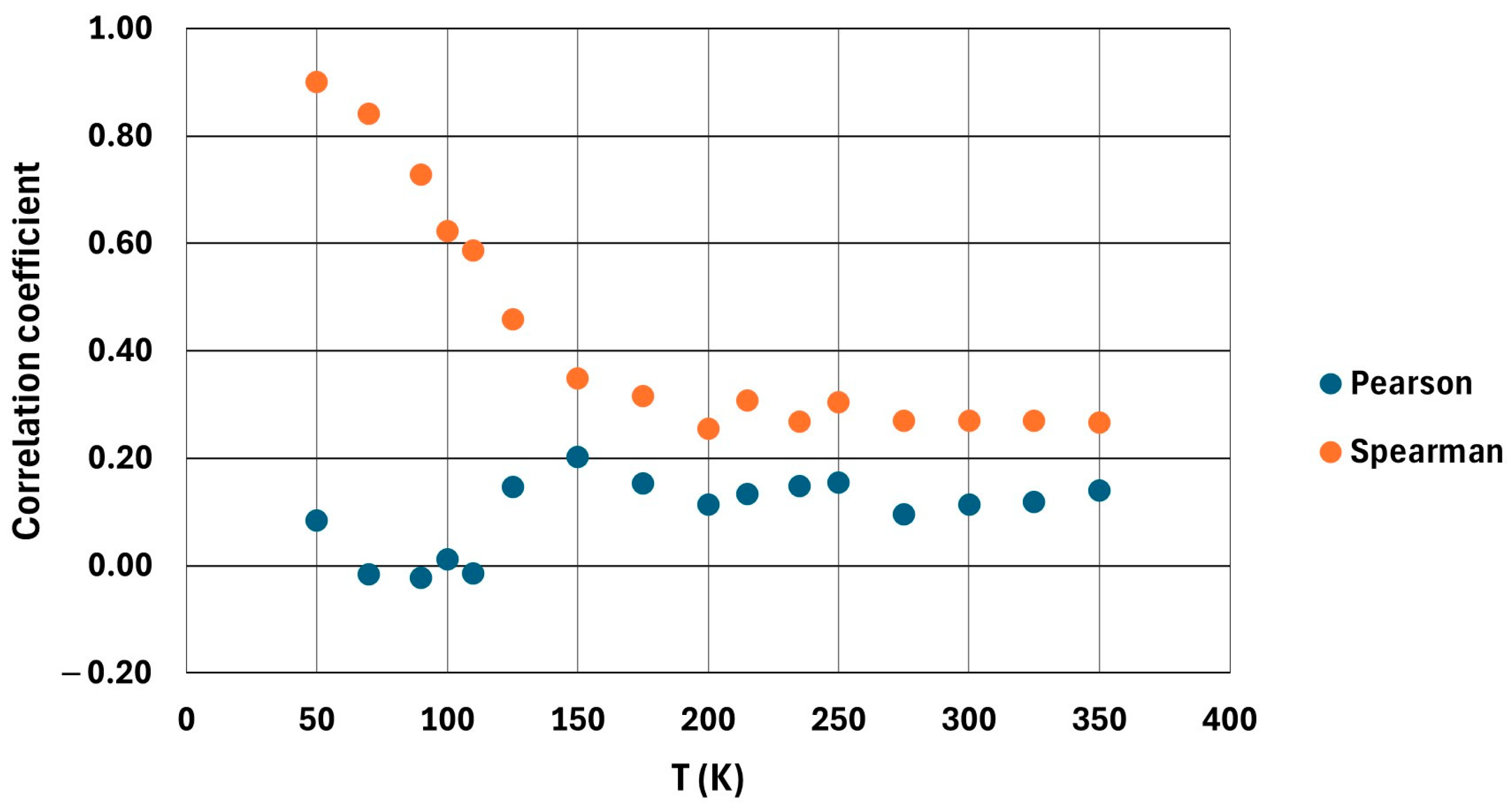
3.1. Correlation Analysis with the Complete Dataset

Table 3. Pearson and Spearman coefficients, number of frames of the MD simulations, and lifetimes. The τ values have been obtained from Table 1 of Ref. [33].

T (K)	Frames	Pearson	Spearman	τ (ps) HBs_C	τ (ps) HBs_N
50	60,000	0.08	0.90	-	-
70	60,000	−0.02	0.84	7.6408	6.6992
90	60,000	−0.02	0.73	3.4374	2.7417
100	60,000	0.01	0.62	2.5533	2.0081
110	60,000	−0.01	0.59	1.5975	1.4053
125	60,000	0.15	0.46	0.7176	0.9616
150	20,000	0.20	0.35	0.5085	0.6800
175	20,000	0.15	0.32	0.3878	0.5150
200	20,000	0.11	0.25	0.3409	0.4166
215	20,000	0.13	0.31	0.3044	0.3830
235	20,000	0.15	0.27	0.2464	0.3383
250	20,000	0.15	0.30	0.2349	0.3188
275	20,000	0.10	0.27	0.2082	0.2787
300	20,000	0.11	0.27	0.1933	0.2532
325	20,000	0.12	0.27	0.1774	0.2267
350	20,000	0.14	0.27	0.1635	0.2035

shows, for each temperature, the total number of MD frames, the HB lifetimes, and the Pearson and Spearman coefficients, considering the initial (before block averaging) dataset. As can be seen in Figure 3, the trends in the Pearson and Spearman coefficients were distinct across the entire temperature range examined (50–350 K). At lower temperatures (≤125 K), the Spearman coefficients presented high values, consistently above 0.5, indicating a possible relationship between the variables analyzed. However, the Pearson coefficient remained low in this range, fluctuating between −0.02 and 0.14.

For T > 125 K, it was observed that Spearman coefficients decreased significantly, with values fluctuating around 0.3. This trend suggests a reduction in the strength of the monotonic correlation between variables at higher temperatures. The Pearson coefficient also showed an upward trend at intermediate temperatures but remained relatively low, indicating that the relationship between the variables remained weakly linear or was influenced by additional factors.

However, it can be observed in Figure 1 that the Pearson and Spearman coefficients at temperatures above 125 K are proportional and both indicate low correlation. In contrast, at lower temperatures, the Pearson and Spearman coefficients are qualitatively different, indicating low and high correlations, respectively. This could indicate two possible situations: either that, at low temperatures, the system is not thermalized, or that the behavior of the data ceases to be linear at low temperatures. This latter behavior might be interpreted as non-linear correlation between both types of HBs. At sufficiently low temperatures, the structure of the system becomes more ordered with less thermal contribution, which facilitates the emergence of HB networks in which the formation or breaking of one type of bond determines the presence of the other.

In this context, a correlation between both types of HBs—as suggested by a high Spearman coefficient—appears plausible. If the formation of an N–H···Br bond forces the cation to adopt a specific orientation, it is reasonable to assume that such orientation also influences the likelihood of forming a C–H···Br bond in the opposite direction and vice versa.

This possible cooperative relationship, although not necessarily linear, could arise from the spatial constraints imposed by the crystal structure and the need to optimize interactions between the organic cation and the inorganic framework. Within the cubo-octahedral cavity of the perovskite lattice, the MA cation is confined by its surrounding Pb₈Br₁₂ environment, which limits its freedom of motion and imposes specific steric and electrostatic conditions. When an N–H···Br bond forms, the resulting orientation of the NH₃⁺ group inevitably repositions the CH₃ end of the cation, potentially placing one or more hydrogen atoms of the methyl group in closer proximity to bromide ions. This geometrical rearrangement may facilitate the formation of a C–H···Br interaction simply due to spatial alignment without requiring a direct energetic coupling between the two types of HBs.

Moreover, from an energetic standpoint, the system may favor configurations that maximize the number of stabilizing interactions within the cavity, even if the individual contributions of C–H···Br bonds are weaker. The presence of multiple simultaneous weak interactions can contribute collectively to the stabilization of the local structure, which may manifest statistically as a monotonic correlation between bond types. Importantly, this scenario does not imply that the formation of one bond directly triggers the other but rather that both emerge as compatible outcomes within a constrained conformational landscape. This subtle form of cooperativity—driven more by spatial accommodation than by direct coupling—could explain the emergence of monotonic patterns in the HB dynamics at low temperatures.

However, due to the marked difference between the Pearson and Spearman coefficients—and, more importantly, the lack of consistency in the high Spearman values (only exceeding 0.8 at 70 K and 50 K)—it becomes necessary to carry out more detailed analyses, as developed in the following sections.

Section 3.2 and Section 3.3 are devoted to analyzing the difference in both types of correlation coefficients.

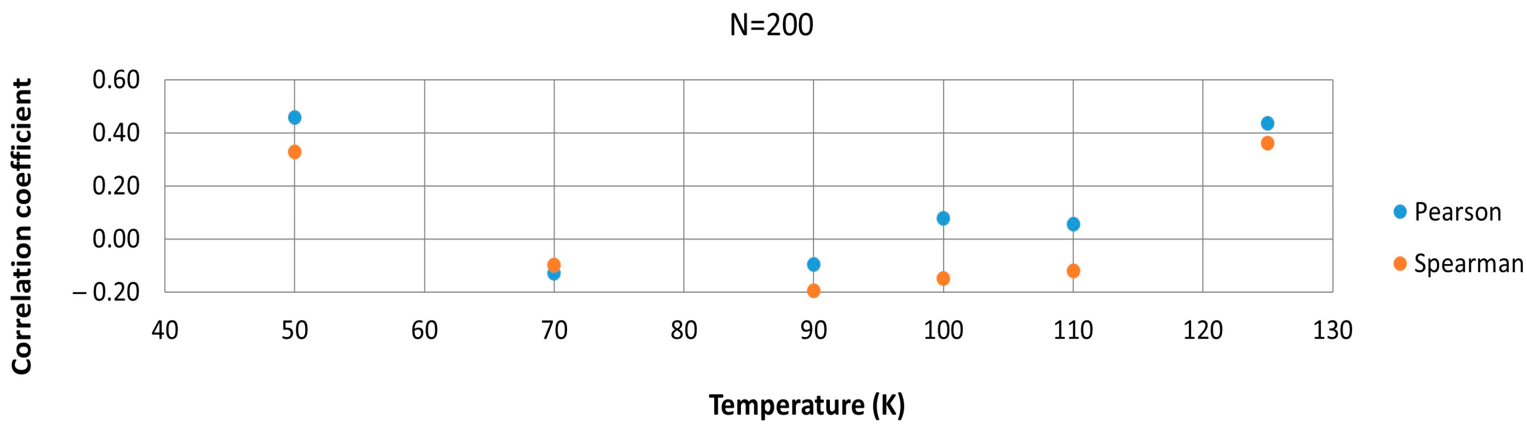
3.2. Correlation Analysis with Fragmented Dataset

To verify that our correlation results accurately reflect equilibrium behavior and are not biased by initial conditions, we recalculated the correlation coefficients using only (later) fragments of each trajectory. Table 1 shows that, at all temperatures, the correlation coefficients exhibit only fluctuations when the dataset is fragmented. Focusing on the low-temperature examples, at 50 K, the Pearson correlation using the full 60,000-frame dataset is $r\approx 0.08$, whereas the Spearman correlation is ρ ≈ 0.90. If, instead, we use only the last 10,000 frames of that trajectory, we obtain $r\approx -0.24$ and ρ ≈ 0.88. Using the last 20,000 frames, we get r ≈ 0.13 and ρ ≈ 0.86, and using the last 50,000 frames, we get r ≈ 0.12 and ρ ≈ 0.89. These values are very close to each other, given the statistical uncertainty (on the order of a few hundredths). The small variations in Pearson’s r at 50 K (some slightly negative, some slightly positive) likely reflect random fluctuations due to the finite sample size rather than a systematic trend. Critically, the Spearman coefficient remains consistently high (0.86–0.90) regardless of segment length and the Pearson coefficient stays close to zero. Similarly, at 70 K, whether we use 10,000 frames or 60,000 frames, Spearman’s ρ remains around 0.8 (0.80–0.84) and Pearson’s r stays between –0.05 and –0.02. At 125 K, using the last 10,000 frames gives ρ ≈ 0.46 and r ≈ 0.12, while using the full 60,000 frames gives ρ ≈ 0.46 and r ≈ 0.15. We see similarly negligible differences for higher temperatures, for example, at 200 K Pearson’s r = 0.11 and Spearman’s ρ = 0.25 for the full 20,000-frame dataset. Even if we only consider the last 5000 frames, we obtain r = 0.15 and ρ = 0.30. In all cases, the direction and qualitative magnitude of the correlation (strong vs. weak, positive vs. negative) remain the same, regardless of the portion of the trajectory analyzed. This consistency across different trajectory segments leads us to conclude that the simulations were indeed well balanced and that the correlation results are not affected by initial unbalanced behavior, as can be observed in Figures S1–S4 of the Supplementary Materials.

3.3. Correlation Analysis with Block-Averaged Dataset

The impact of data averaging was systematically assessed by analyzing correlation coefficients for different subset sizes. The results demonstrated that as the dataset was averaged into smaller subsets (e.g., 400, 60, and 20 data points per temperature), the fluctuations in correlation coefficients were reduced. This suggests that averaging effectively minimized statistical noise while preserving the overall trend of the correlation.

Scatter plots representing the correlation coefficients across different averaging levels confirmed that smaller sample sizes introduced variability in the results.

It is worth noting that for 2000-element block-averaged sets, the Spearman coefficient is higher than that of the other block-averaged set sizes across all temperatures. This leads us to conclude that, as with the complete data series, there is still too much statistical “noise”. Regarding the case of 50 K, the values show significant fluctuations for all subsets, which suggests that the total number of data points is not large enough to properly analyze the system’s behavior.

Finally, it should be noted that, as can be seen in Figure 4 and Figure 5, for subset sizes of 200 and 400 data points per temperature, the qualitative discrepancies between the Pearson and Spearman coefficients were eliminated, and this can be considered the ideal size range for analyzing correlations. This circumstance, as well as the deviations in the other cases analyzed, can be observed in detail in Figures S5–S12 of the Supplementary Materials.

4. Discussion

The statistical analysis of HB formation in CH₃NH₃PbBr₃ across 50–350 K indicates that no clear correlation exists between N–H···Br and C–H···Br HBs. Initial observations showed a stark contrast between Spearman and Pearson correlation coefficients at low temperatures. At 50 K, the Spearman rank correlation coefficient (ρ) between the occurrences of N–H···Br and C–H···Br was very high (~0.9), whereas the Pearson coefficient remained near zero.

This suggests that while a strong monotonic association seemed to be present at 50 K (i.e., as one type of bond increased, the other type tended to increase as well), there was no linear relationship. Similar behavior was observed up to ~125 K: Spearman’s ρ remained above 0.5 in this range, yet Pearson’s r fluctuated between −0.02 and 0.14.

Such disparity implies that any apparent correlation at low temperatures was non-linear in nature. For higher temperatures (T > 125 K), however, even the Spearman coefficient dropped to around 0.3.

However, further scrutiny reveals that the apparent strong correlation at 50 K is not statistically robust. When the 50 K dataset was examined in fragmented segments and through block-averaging techniques, the correlation metrics showed pronounced instability. In a fragmented analysis of the 50 K trajectory, the Spearman coefficient was found to fluctuate significantly between different time intervals instead of remaining consistently high. This variability signals that the high ρ value from the full dataset may be an artifact of the discreteness of the number of HBs rather than evidence of a persistent coupling between N–H···Br and C–H···Br formations. Likewise, a block-averaging approach caused the initially high Spearman correlation at 50 K to collapse. For example, reducing the 50 K dataset by averaging into blocks of 200 points caused ρ to drop from ~0.90 to ~0.33.

With more extreme averaging (yielding very few data points per set), the correlation continued to dwindle toward negligible values, underscoring the fragility of the observed association. These outcomes demonstrate that the strong monotonic correlation seen at 50 K is not maintained under resampling; instead, it is highly sensitive to data handling and likely driven by transient or coincidental alignments in the dataset. In line with this, even a modest change in the number of frames considered at 50 K led to noticeable changes (and even sign inversions) in the Pearson coefficient, further highlighting the unreliability of any inferred correlation at this temperature. The conclusion of the averaged and segmented analyses is clear: The supposed correlation between N–H···Br and C–H···Br HBs at low temperatures is not robust or representative.

Considering the entire temperature spectrum, the results consistently indicate that N–H···Br and C–H···Br form independently. At none of the investigated temperatures is there a statistically consistent relationship. This shows that the formation of one type of HB does not influence the formation of the other type. The lack of a dependable correlation suggests that each HB type is governed by its own local geometric and energetic factors without a coordinated interplay. In practical terms, the methylammonium cation’s N–H and C–H groups do not exhibit cooperative hydrogen-bonding behavior—the occurrence of an N–H···Br bond does not measurably make a C–H···Br bond more (or less) likely and vice versa. This independence can be rationalized by the perovskite’s structure: the CH₃NH₃ cation has multiple degrees of freedom and can orient and reorient within the cage of PbBr₆ octahedra, often engaging one or both types of HBs stochastically rather than synergistically. Indeed, one might expect that if the ammonium end (NH₃⁺) is involved in a strong N–H···Br interaction, the orientation could either favor or hinder a C–H···Br contact; however, our statistical analysis finds no consistent pattern of such coupling. Each type of HB can form or break independently of the other, governed by thermal fluctuations and instantaneous local arrangements of the cation and the surrounding anions.

It should be noted that the behavioral change observed at 125 K coincides with the structural transition from tetragonal to orthorhombic in CH₃NH₃PbBr₃. This transition marks a shift in the dynamic capacity of the cation, leading to greater freedom of re-orientation and resulting in more disordered HB formation. Moreover, 125 K is the lowest temperature for which we have observed relative rotation of the CH₃ and NH₃ groups, as inferred from the time dependence of the dihedral angle H–N–C–H shown in Figure S13 of the Supplementary Materials. Consequently, any residual monotonic relationship between N–H···Br and C–H···Br interactions observed at low temperatures no longer persists at higher temperatures. This reinforces the conclusion that the apparent correlation below 125 K is not due to an intrinsic coupling between these interactions but rather to the constraints imposed by the low-temperature crystal structure.

Finally, it should be noticed that correlation and causality are not the same phenomenon, although they are frequently difficult to distinguish. If the formation or breaking of C–H···Br bonds were caused by the formation of breaking of N–H···Br bonds, one could study the correlation between the corresponding data after applying a time shift. Our study considers no time delay, which is consistent with a rigid MA molecule view. The study could be extended considering time delay of the order of MA vibration period (10–40 fs). However, these times are one or two orders of magnitude smaller than the HB lifetimes (Table 3). Hence, we think that a causal relationship would manifest in the correlation analysis carried out in this work.

5. Conclusions

Our investigation of the correlation between C–H···Br and N–H···Br HBs in CH₃NH₃PbBr₃ concludes the following points:

• No definitive correlation was found between N–H···Br and C–H···Br formations over the temperature range studied. The analysis shows that the occurrences of N-type and C-type HBs are uncorrelated, indicating that these two types of interactions form and fluctuate independently throughout the simulations.
• The initially high Spearman correlation observed at 50 K is neither reliable nor representative of a true coupling between the two types of HB. While a Spearman ρ ≈ 0.9 at 50 K suggested a possible monotonic relationship, this turned out to be an artifact of limited sampling and specific conditions. When examining the 50 K data more rigorously, dividing them into shorter segments, and averaging/blocking the data points, the correlation coefficients varied considerably and often approached zero. This instability implies that the apparent 50 K correlation cannot be considered statistically robust or significant.
• A clear change in Spearman coefficient behavior is observed around 125 K, which coincides with the system’s phase transition region. This point marks the transition from a possible monotonic correlation at low temperatures to a weak or negligible correlation at higher temperatures, suggesting that the structural reorganization associated with the phase change affects the dynamics of HB.

The observed independence of N–H···Br and C–H···Br HBs implies that future studies and models can treat these interactions separately. In molecular dynamics simulations, for example, N–H···Br and C–H···Br HBs should be tracked as distinct parameters, since a change in one does not predict a change in the other. This perspective simplifies the interpretation of structural dynamics in hybrid perovskites: Any stability or phase behavior associated with hydrogen bonding must consider the contributions of N–H···Br and C–H···Br individually rather than assuming a combined effect.

References

1. Tao, S.; Schmidt, I.; Brocks, G.; Jiang, J.; Tranca, I.; Meerholz, K.; Olthof, S. Absolute Energy Level Positions in Tin- and Lead-Based Halide Perovskites. Nat. Commun. 2019, 10, 2560. [Google Scholar] [CrossRef] [PubMed]
2. Jellicoe, T.C.; Richter, J.M.; Glass, H.F.J.; Tabachnyk, M.; Brady, R.; Dutton, S.E.; Rao, A.; Friend, R.H.; Credgington, D.; Greenham, N.C.; et al. Synthesis and Optical Properties of Lead-Free Cesium Tin Halide Perovskite Nanocrystals. J. Am. Chem. Soc. 2016, 138, 2941–2944. [Google Scholar] [CrossRef]
3. Savill, K.J.; Ulatowski, A.M.; Herz, L.M. Optoelectronic Properties of Tin–Lead Halide Perovskites. ACS Energy Lett. 2021, 6, 2413–2426. [Google Scholar] [CrossRef] [PubMed]
4. Wang, J.; Yang, C.; Chen, H.; Lv, M.; Liu, T.; Chen, H.; Xue, D.-J.; Hu, J.-S.; Han, L.; Yang, S.; et al. Oriented Attachment of Tin Halide Perovskites for Photovoltaic Applications. ACS Energy Lett. 2023, 8, 1590–1596. [Google Scholar] [CrossRef]
5. Kaiser, W.; Ricciarelli, D.; Mosconi, E.; Alothman, A.A.; Ambrosio, F.; De Angelis, F. Stability of Tin- versus Lead-Halide Perovskites: Ab Initio Molecular Dynamics Simulations of Perovskite/Water Interfaces. J. Phys. Chem. Lett. 2022, 13, 2321–2329. [Google Scholar] [CrossRef]
6. Seo, J.; Noh, J.H.; Seok, S. Il Rational Strategies for Efficient Perovskite Solar Cells. Acc. Chem. Res. 2016, 49, 562–572. [Google Scholar] [CrossRef]
7. Kojima, A.; Teshima, K.; Shirai, Y.; Miyasaka, T. Organometal Halide Perovskites as Visible-Light Sensitizers for Photovoltaic Cells. J. Am. Chem. Soc. 2009, 131, 6050–6051. [Google Scholar] [CrossRef]
8. Khadka, D.B.; Shirai, Y.; Yanagida, M.; Ryan, J.W.; Song, Z.; Barker, B.G.; Dhakal, T.P.; Miyano, K. Advancing Efficiency and Stability of Lead, Tin, and Lead/Tin Perovskite Solar Cells: Strategies and Perspectives. Solar RRL 2023, 7, 2300535. [Google Scholar] [CrossRef]
9. NREL Chart on Record Cell Efficiencies. Available online: https://www.nrel.gov/pv/cell-efficiency.html (accessed on 23 April 2025).
10. Zhu, M.; Cao, G.; Zhou, Z. Recent Progress toward Highly Efficient Tin-Based Perovskite (ASnX3) Solar Cells. Nano Select 2021, 2, 1023–1054. [Google Scholar] [CrossRef]
11. Kim, J.Y.; Lee, J.-W.; Jung, H.S.; Shin, H.; Park, N.-G. High-Efficiency Perovskite Solar Cells. Chem. Rev. 2020, 120, 7867–7918. [Google Scholar] [CrossRef] [PubMed]
12. Wang, T.; Hao, Y.; Zhu, M.; Cao, G.; Zhou, Z. Hydrogen Bonds in Perovskite for Efficient and Stable Photovoltaic . Chin. J. Chem. 2024, 42, 1284–1306. [Google Scholar] [CrossRef]
13. Gu, S.; Lin, R.; Han, Q.; Gao, Y.; Tan, H.; Zhu, J. Tin and Mixed Lead–Tin Halide Perovskite Solar Cells: Progress and Their Application in Tandem Solar Cells. Adv. Mater. 2020, 32, 1907392. [Google Scholar] [CrossRef]
14. Ramadan, A.J.; Oliver, R.D.J.; Johnston, M.B.; Snaith, H.J. Methylammonium-Free Wide-Bandgap Metal Halide Perovskites for Tandem Photovoltaics. Nat. Rev. Mater. 2023, 8, 822–838. [Google Scholar] [CrossRef]
15. Aktas, E.; Rajamanickam, N.; Pascual, J.; Hu, S.; Aldamasy, M.H.; Di Girolamo, D.; Li, W.; Nasti, G.; Martínez-Ferrero, E.; Wakamiya, A.; et al. Challenges and Strategies toward Long-Term Stability of Lead-Free Tin-Based Perovskite Solar Cells. Commun. Mater. 2022, 3, 104. [Google Scholar] [CrossRef]
16. McGovern, L.; Futscher, M.H.; Muscarella, L.A.; Ehrler, B. Understanding the Stability of MAPbBr3 versus MAPbI3: Suppression of Methylammonium Migration and Reduction of Halide Migration. J. Phys. Chem. Lett. 2020, 11, 7127–7132. [Google Scholar] [CrossRef]
17. Liu, C.; Yang, Y.; Chen, H.; Xu, J.; Liu, A.; Bati, A.S.R.; Zhu, H.; Grater, L.; Hadke, S.S.; Huang, C.; et al. Bimolecularly Passivated Interface Enables Efficient and Stable Inverted Perovskite Solar Cells. Science 2023, 382, 810–815. [Google Scholar] [CrossRef]
18. Li, T.; Xu, J.; Lin, R.; Teale, S.; Li, H.; Liu, Z.; Duan, C.; Zhao, Q.; Xiao, K.; Wu, P.; et al. Inorganic Wide-Bandgap Perovskite Subcells with Dipole Bridge for All-Perovskite Tandems. Nat. Energy 2023, 8, 610–620. [Google Scholar] [CrossRef]
19. Zhao, Y.; Heumueller, T.; Zhang, J.; Luo, J.; Kasian, O.; Langner, S.; Kupfer, C.; Liu, B.; Zhong, Y.; Elia, J.; et al. A Bilayer Conducting Polymer Structure for Planar Perovskite Solar Cells with over 1,400 Hours Operational Stability at Elevated Temperatures. Nat. Energy 2021, 7, 144–152. [Google Scholar] [CrossRef]
20. Li, G.; Su, Z.; Canil, L.; Hughes, D.; Aldamasy, M.H.; Dagar, J.; Trofimov, S.; Wang, L.; Zuo, W.; Jerónimo-Rendon, J.J.; et al. Highly Efficient P-i-n Perovskite Solar Cells That Endure Temperature Variations. Science 2023, 379, 399–403. [Google Scholar] [CrossRef]
21. Li, C.; Wang, X.; Bi, E.; Jiang, F.; Park, S.M.; Li, Y.; Chen, L.; Wang, Z.; Zeng, L.; Chen, H.; et al. Rational Design of Lewis Base Molecules for Stable and Efficient Inverted Perovskite Solar Cells. Science 2023, 379, 690–694. [Google Scholar] [CrossRef]
22. Bai, S.; Da, P.; Li, C.; Wang, Z.; Yuan, Z.; Fu, F.; Kawecki, M.; Liu, X.; Sakai, N.; Wang, J.T.-W.; et al. Planar Perovskite Solar Cells with Long-Term Stability Using Ionic Liquid Additives. Nature 2019, 571, 245–250. [Google Scholar] [CrossRef] [PubMed]
23. Doherty, T.A.S.; Nagane, S.; Kubicki, D.J.; Jung, Y.-K.; Johnstone, D.N.; Iqbal, A.N.; Guo, D.; Frohna, K.; Danaie, M.; Tennyson, E.M.; et al. Stabilized Tilted-Octahedra Halide Perovskites Inhibit Local Formation of Performance-Limiting Phases. Science 2021, 374, 1598–1605. [Google Scholar] [CrossRef] [PubMed]
24. Tavakoli, M.M.; Bi, D.; Pan, L.; Hagfeldt, A.; Zakeeruddin, S.M.; Grätzel, M. Adamantanes Enhance the Photovoltaic Performance and Operational Stability of Perovskite Solar Cells by Effective Mitigation of Interfacial Defect States. Adv. Energy Mater. 2018, 8, 1800275. [Google Scholar] [CrossRef]
25. Saleh, G.; Biffi, G.; Di Stasio, F.; Martín-García, B.; Abdelhady, A.L.; Manna, L.; Krahne, R.; Artyukhin, S. Methylammonium Governs Structural and Optical Properties of Hybrid Lead Halide Perovskites through Dynamic Hydrogen Bonding. Chem. Mater. 2021, 33, 8524–8533. [Google Scholar] [CrossRef]
26. Ibaceta-Jaña, J.; Chugh, M.; Novikov, A.S.; Mirhosseini, H.; Kühne, T.D.; Szyszka, B.; Wagner, M.R.; Muydinov, R. Do Lead Halide Hybrid Perovskites Have Hydrogen Bonds? J. Phys. Chem. C. 2022, 126, 16215–16226. [Google Scholar] [CrossRef]
27. Maity, S.; Verma, S.; Ramaniah, L.M.; Srinivasan, V. Deciphering the Nature of Temperature-Induced Phases of MAPbBr3 by Ab Initio Molecular Dynamics. Chem. Mater. 2022, 34, 10459–10469. [Google Scholar] [CrossRef]
28. Svane, K.L.; Forse, A.C.; Grey, C.P.; Kieslich, G.; Cheetham, A.K.; Walsh, A.; Butler, K.T. How Strong Is the Hydrogen Bond in Hybrid Perovskites? J. Phys. Chem. Lett. 2017, 8, 6154–6159. [Google Scholar] [CrossRef]
29. Garrote-Márquez, A.; Lodeiro, L.; Suresh, R.; Cruz Hernández, N.; Grau-Crespo, R.; Menéndez-Proupin, E. Hydrogen Bonds in Lead Halide Perovskites: Insights from Ab Initio Molecular Dynamics. J. Phys. Chem. C 2023, 127, 15901–15910. [Google Scholar] [CrossRef]
30. Arunan, E.; Desiraju, G.R.; Klein, R.A.; Sadlej, J.; Scheiner, S.; Alkorta, I.; Clary, D.C.; Crabtree, R.H.; Dannenberg, J.J.; Hobza, P.; et al. Defining the Hydrogen Bond: An Account (IUPAC Technical Report). Pure Appl. Chem. 2011, 83, 1619–1636. [Google Scholar] [CrossRef]
31. Arunan, E.; Desiraju, G.R.; Klein, R.A.; Sadlej, J.; Scheiner, S.; Alkorta, I.; Clary, D.C.; Crabtree, R.H.; Dannenberg, J.J.; Hobza, P.; et al. Definition of the Hydrogen Bond (IUPAC Recommendations 2011). Pure Appl. Chem. 2011, 83, 1637–1641. [Google Scholar] [CrossRef]
32. Varadwaj, P.R.; Varadwaj, A.; Marques, H.M.; Yamashita, K. Significance of Hydrogen Bonding and Other Noncovalent Interactions in Determining Octahedral Tilting in the CH3NH3PbI3 Hybrid Organic-Inorganic Halide Perovskite Solar Cell Semiconductor. Sci. Rep. 2019, 9, 50. [Google Scholar] [CrossRef] [PubMed]
33. Garrote-Márquez, A.; Lodeiro, L.; Hernández, N.C.; Liang, X.; Walsh, A.; Menéndez-Proupin, E. Picosecond Lifetimes of Hydrogen Bonds in the Halide Perovskite CH3NH3PbBr3. J. Phys. Chem. C 2024, 128, 20947–20956. [Google Scholar] [CrossRef]
34. Brehm, M.; Thomas, M.; Gehrke, S.; Kirchner, B. TRAVIS—A Free Analyzer for Trajectories from Molecular Simulation. J. Chem. Phys. 2020, 152, 164105. [Google Scholar] [CrossRef]
35. Humphrey, W.; Dalke, A.; Schulten, K. VMD: Visual Molecular Dynamics. J. Mol. Graph. 1996, 14, 33–38. [Google Scholar] [CrossRef]
36. Lange, O.F.; Grubmüller, H. Full Correlation Analysis of Conformational Protein Dynamics. Proteins 2008, 70, 1294–1312. [Google Scholar] [CrossRef] [PubMed]
37. Diez, G.; Nagel, D.; Stock, G. Correlation-Based Feature Selection to Identify Functional Dynamics in Proteins. J. Chem. Theory Comput. 2022, 18, 5079–5088. [Google Scholar] [CrossRef]
38. Nagel, D.; Diez, G.; Stock, G. Accurate Estimation of the Normalized Mutual Information of Multidimensional Data. J. Chem. Phys. 2024, 161, 054108. [Google Scholar] [CrossRef] [PubMed]
39. McClendon, C.L.; Friedland, G.; Mobley, D.L.; Amirkhani, H.; Jacobson, M.P. Quantifying Correlations Between Allosteric Sites in Thermodynamic Ensembles. J. Chem. Theory Comput. 2009, 5, 2486–2502. [Google Scholar] [CrossRef]
40. Weaver, K.F.; Morales, V.; Dunn, S.L.; Godde, K.; Weaver, P.F. Pearson’s and Spearman’s Correlation. In An Introduction to Statistical Analysis in Research; Weaver, K.F., Morales, V., Dunn, S.L., Godde, K., Weaver, P.F., Eds.; Wiley: Hoboken, NJ, USA, 2017. [Google Scholar] [CrossRef]
41. Xiao, C.; Ye, J.; Esteves, R.M.; Rong, C. Using Spearman’s Correlation Coefficients for Exploratory Data Analysis on Big Dataset. Concurr. Comput. 2016, 28, 3866–3878. [Google Scholar] [CrossRef]
42. Nosé, S. A Molecular Dynamics Method for Simulations in the Canonical Ensemble. Mol. Phys. 1984, 52, 255–268. [Google Scholar] [CrossRef]
43. Kresse, G.; Furthmüller, J. Efficient Iterative Schemes for Ab Initio Total-Energy Calculations Using a Plane-Wave Basis Set. Phys. Rev. B 1996, 54, 11169–11186. [Google Scholar] [CrossRef] [PubMed]
44. Liang, X.; Klarbring, J.; Baldwin, W.J.; Li, Z.; Csányi, G.; Walsh, A. Structural Dynamics Descriptors for Metal Halide Perovskites. J. Phys. Chem. C 2023, 127, 19141–19151. [Google Scholar] [CrossRef] [PubMed]
45. Zhou, S.; Liu, Y.; Wang, S.; Wang, L. Effective Prediction of Short Hydrogen Bonds in Proteins via Machine Learning Method. Sci. Rep. 2022, 12, 469. [Google Scholar] [CrossRef] [PubMed]
Figure 1. A unit cell of CH3NH3PbBr3, showing two X–H···Y hydrogen bonds (N–H···Br and C–H···Br) as dotted lines, as well as the X–Y distances (dashed lines and values) and the X–H–Y angles that define them.
Solids 06 00029 g001
Figure 3. Values of the Pearson and Spearman coefficients as a function of temperature.
Solids 06 00029 g003
Figure 4. Values of the Pearson and Spearman coefficients for T ≤ 125 K for a set size of 400.
Solids 06 00029 g004
Figure 5. Values of the Pearson and Spearman coefficients for T ≤ 125 K for a set size of 200.
Solids 06 00029 g005