Experimental Evaluation of Temperature and Strain-Rate-Dependent Mechanical Properties of Austenitic Stainless Steel SS316LN and a New Methodology to Evaluate Parameters of Johnson–Cook and Ramberg–Osgood Material Models

Abstract

Austenitic stainless steel SS316LN is used as the material of construction of the vessel and core components of fast breeder reactors, which operate at an elevated temperature of 550 °C. For design and integrity analysis using the finite element method, material models, such as Johnson–Cook and Ramberg–Osgood, are widely used. However, the temperature- and strain-rate-dependent plasticity and damage parameters of these models for this material are not available in the literature. Moreover, the method of evaluation of temperature and strain-rate-dependent plasticity parameters, in literature, has some major shortcomings, which have been addressed in this work. In addition, a new optimization-based procedure has been developed to evaluate all nine plasticity and damage parameters, which uses results of combined finite element analysis and experimental data. The procedure has been validated extensively by testing tensile specimens at different temperatures, by testing notched tensile specimens of different notch radii, and by carrying out high strain-rate tests using a split Hopkinson pressure bar test setup. The parameters of the Johnson–Cook material model, evaluated in this work, have been used in finite element analysis to simulate load-displacement behavior and fracture strains of various types of specimens, and the results have been compared with experimental data in order to check the accuracy of the parameters. The procedure developed in this work shall help the researchers to adopt such a technique for accurate estimation of both plasticity and damage parameters of different types of material models.

1. Introduction

The major components of the reactor assembly in the Prototype Fast Breeder Reactor (PFBR), such as the grid plate, core support structure, main vessel, inner vessel, and intermediate heat exchanger, are made of austenitic stainless steel grade 316LN (SS316LN) [1]. These components are usually exposed to high temperatures during reactor operation and are submerged in a molten metal atmosphere (i.e., molten sodium). PFBR uses molten metallic sodium (500–550 °C) as coolant, and this subjects the material of the core components (including the vessel) to high thermal stresses due to the high convective heat transfer coefficient of molten sodium. SS316LN is the preferred structural material because it is a low-carbon steel grade that avoids sensitization during welding, preventing stress corrosion cracking in the chloride-rich environments of coastal sites. SS316LN also exhibits excellent mechanical properties, including tensile strength, creep resistance, low-cycle fatigue, creep-fatigue interaction, and high-cycle fatigue strength at both low and high temperatures [2].

For design by analysis, the reactor components are designed using standard codes, which have been developed by the American Society of Mechanical Engineers (ASME) and French engineers. Among these codes, the RCC-MR code [3] is a predominant French design code, which is used for the design of components of fast breeder reactors. This code provides design curve equations for the stress-strain relationship at various temperatures for SS316LN; however, these are valid for up to 1.5% plastic strain only. The design curve expressions as provided in the RCC-MR code are not valid if the plastic strain exceeds 1.5%. Higher plastic strains can occur in regions of the structure with large geometrical discontinuities, such as shell-nozzle junctions, vessel heads, T-junctions, etc. Typically, the design procedure uses the lower-bound stress-strain curve; however, the life or integrity assessment techniques use the median value of the stress-strain curve. This indicates that different approaches are needed while carrying out design and safety analysis of the reactor components.

High-temperature properties of SS316LN are essential for integrity analysis of reactor components during severe accident scenarios. The postulated Core Disruptive Accident (CDA) is one such accident, which occurs due to the melting of nuclear fuel in the reactor core. This can lead to a significant rise in the temperature of the coolant and the structural material (of the order of 1000 °C). At elevated temperatures, significant changes in the strength and ductility of SS316LN stainless steel occur. Hence, the properties of the structural materials need to be evaluated at different temperatures and incorporated in an appropriate material constitutive model for finite element analysis in order to demonstrate that the reactor core is safe during CDA and other such postulated severe accidents.

The postulated CDA can also impart shock loads on structural components. For analysis of these scenarios, a rate-dependent material model is essential for structural integrity analysis of reactor assembly components, especially the main vessel. However, the RCC-MR code [3] neither provides rate-dependent stress-strain data nor the parameter of material constitutive models such as those of Johnson–Cook [4]. For thermo-mechanical analysis of structural components, where temperature varies across the thickness of the component, temperature-dependent material stress-strain data, provided in the form of true stress-strain curves, are essential input data for the analysis, and it is one of the approaches in finite element analysis. On the other hand, the use of the temperature and strain-rate-dependent Johnson–Cook model is more elegant, as it models both the plastic hardening behavior and softening behavior due to the incorporation of a damage parameter. It takes care of the coupled effect of damage softening, thermal softening, strain hardening, and strain rate hardening phenomena on the material deformation behavior.

In this work, the temperature and strain-rate-dependent plasticity and damage parameters of the Johnson–Cook material model for austenitic grade stainless steel SS316LN are evaluated by following a new procedure, where both experimental data and results of finite element (FE) analysis have been used. The parameters evaluated through this procedure have been validated extensively using data from both smooth and notched tensile specimens at different temperatures. In addition, the parameters of the Ramberg–Osgood material model in the range of 25–650 °C have been evaluated for SS316LN using optimization algorithms, which take into account both experimental data and FE analysis results of smooth as well as notched tensile specimens.

This paper has been divided into eight sections. After a brief introduction to the problem in Section 1, the relevant literature is discussed in Section 2. The details of material composition, specimen design, experimental procedure, test data, and mechanical properties of SS316LN stainless steel at different temperatures have been presented in Section 3. The conventional procedure (as available in the literature) and the new algorithm for the evaluation of plastic hardening parameters of both Johnson–Cook and Ramberg–Osgood models are provided in Section 4 and Section 5, respectively. The procedure for the evaluation of damage parameters of the Johnson–Cook material model is presented in Section 6, followed by a discussion and validation of results in Section 7. The paper ends with an outlining of the concluding remarks in Section 8.

2. Brief Review of Literature

2.1. Literature on Microstructure, Mechanical, Fatigue, Creep, and Fracture Properties of SS316LN

Austenitic grade stainless steel SS316LN is used in both fission and fusion-type reactors for the manufacturing of their components due to its excellent corrosion resistance and mechanical and fracture properties in both cryogenic and elevated temperature environments. In an international thermonuclear experimental reactor (ITER), SS316LN is used as the material for cryogenic jackets and the central solenoid [5]. The metallurgical and mechanical properties of two grades of austenitic stainless steels used as material for the conductor jacket of the ITER central solenoid have been presented in Ref. [5]. The tensile test data of SS 316LN jacket material are presented in Ref. [6]. The effects of cryo-rolling and other methods of plastic pre-straining on the change in microstructure, mechanical, and fracture properties of SS316LN steel have been studied extensively in the literature [7,8,9,10,11,12,13,14].

The influence of thermo-mechanical processing conditions on the mechanical properties of SS316LN steel has been studied and presented in Kvackaj et al. 2020 [15]. Stress corrosion cracking of SS316LN stainless steel in the primary water environment of ITER and the ratcheting-induced twinning/de-twinning behavior is studied in Refs. [16,17], respectively. Different methods have been employed in the literature to modify and enhance the properties of austenitic grades of stainless steel, such as spray forming [18], surface mechanical attrition treatment [19], heat treatment [20,21], etc.

Recently, different types of novel manufacturing techniques (metal powder injection molding [22], direct energy deposition [23], additive manufacturing [24], etc.) have been developed, which are fast, efficient, and suitable to tailor the mechanical and fracture properties of austenitic stainless steel components. A comparative analysis of the mechanical properties of SS316L, as obtained through conventional and additive manufacturing techniques, has been presented in Ref. [25]. A review of the processing techniques, microstructure, properties, and performance of austenitic-grade stainless steels at high temperatures is presented in Ref. [26].

Another important aspect that is investigated in the literature in the study of the high-temperature deformation behavior of austenitic grade stainless steel is its microstructure instabilities. Way back in 1972, Weiss and Stickler [27] studied the phase instabilities in the microstructure of SS316 grade austenitic stainless steel during its high-temperature exposure. Later, several authors [28,29,30,31,32,33] reported precipitation of different types of intermetallic compounds and brittle phases (e.g., σ, χ, η) in the matrix, especially when the temperature exceeds 650 °C, which can alter the mechanical and fracture properties of these grades of materials.

Studies involving the evaluation of tensile and fracture properties of austenitic grade stainless steel SS316LN are very limited in the literature, especially when the high temperature and rate-dependent mechanical and fracture properties are concerned. However, extensive literature exists regarding creep [34,35], time-dependent deformation behavior [36], low cycle fatigue property evaluation [37,38,39], thermal and thermo-mechanical fatigue [40,41,42], multi-axial low cycle fatigue [40,42], mechanical and thermo-mechanical fatigue crack growth [43,44], and the effect of strain rate on low cycle fatigue crack growth [45] of the above grade of stainless steel. Constitutive modeling of creep [46], cyclic deformation [47], and hardening behavior of austenitic grades of stainless steels have also been presented in the literature [48]. A modeling technique involving first-principles simulations has been presented by Li et al. [49], which has been used to study the evolution of defect structure in the material. The effect of defect structure on the mechanical properties of SS316LN stainless steel is also studied in Ref. [49]. The fracture properties of austenitic grades of stainless steel are presented in Refs. [50,51,52,53]. The mechanism of the fracture process in a cryogenic temperature environment has also been studied for SS316LN laser welded joints in Ref. [53]. The ball indentation technique has been used by Kumar et al. [54] and Ragavendran et al. [55] to evaluate the tensile properties of thermally aged 316LN stainless steel with varying nitrogen content and welded joints, respectively. The effect of hydrogen on the tensile property and strain rate-dependent property of SS316L stainless steel has been studied in Refs. [56,57].

2.2. Literature on Damage Models for Simulation of Ductile Fracture

There exist several damage models in the literature, that describe the process of ductile damage development in the material, the damage parameter being a function of localized strain and stress field for a given material point, in terms of either void volume fraction ‘f’ or a damage parameter ‘D’. Popular among these are a class of Gurson-Tvergaard-Needleman (GTN) models and their subsequent modifications [58,59]. The other class of models uses a damage parameter ‘D’, and this is coupled to the effective stress field through the parameter (1 − D), where ‘D = 0’ corresponds to the undamaged state and ‘D = 1’ corresponds to the damaged state of the material.

The development of damage depends upon several parameters such as stress triaxiality, the Lode parameter, temperature, strain rate, etc. Lemaitre [60] proposed such a coupled model in 1982 using the parameter ‘D’. In this model, both the yield function and the damage dissipation potentials are coupled to the evolution of the parameter ‘D’, which changes with the state of material deformation. Takuda et al. [61] used the damage parameter to predict the forming limit in the bore-expanding process of sheet metals. He has used the limiting strain plastic values (as a function of stress triaxiality) to define the ductile fracture criterion. Later, Bao and Wierzbicki [62,63] generalized this approach and defined a fracture locus in the equivalent strain and stress triaxiality space to model the fracture process.

Bai and Wierzbicki [64] developed a new metal plasticity and fracture model considering both pressure and Lode parameter dependence of the yield surface and dissipation potential function. Later, a modified Mohr–Coulomb model was also presented by Bai and Wierzbicki [65], which can be used to simulate the ductile fracture process in metals. Later, an extension of the modified Bai–Wierzbicki model for predicting ductile fracture under complex loading conditions was presented by Wu et al. [66]. A 2D Lode improved Lemaitre’s ductile damage model was also presented by Nezhad and Aboutalebi [67], and it was implemented to model the fracture of sheet metals for various types of loading conditions. Several ductile damage models, which use ‘D’ as a damage parameter (several functional forms of ‘D’ for its dependence on various parameters such as stress triaxiality, temperature, etc., were proposed by various researchers), were used in the literature [68,69,70,71,72,73] to predict the failure of sheet metals used in several processes such as deep drawing [70], shearing of a stud [71], strip tearing during cold rolling [72], etc.

2.3. Rationale for Choice of Johnson–Cook and Ramberg–Osgood Models in This Work

The Johnson–Cook model [4] has been used in this work for its simplicity and ease of evaluation of both plasticity (A, B, n, C, and m) as well as the damage parameters (d₁ to d₅), directly from experimental data. On the other hand, the procedure for evaluation of parameters of other damage models, such as those of GTN [58] and Bai and Wierzbicki [64], etc., needs various types of advanced parameter identification procedures, and many times, only experimental data are inadequate for this purpose. One needs to use several calibration processes to obtain a unique set of parameters. Secondly, the parameters of the Ramberg–Osgood material model (i.e., ‘n’ and ‘α’) are popularly used in closed-form solutions and estimation schemes [74,75], such as those provided by the Electric Power Research Institute (EPRI), USA. These schemes are useful for the evaluation of J-integral, crack mouth opening displacement, load-line displacement, and other such crack-tip loading parameters, which are essential for the integrity analysis of components using fracture mechanics principles. Hence, this model has been used in this work.

2.4. Summary of Literature Survey, Gap Areas, and Objective of This Research

In summary, it can be said that several studies exist in the literature involving creep, low cycle fatigue, and fracture properties of different grades of austenitic stainless steels such as SS316L and SS316LN. The literature involving temperature and strain-rate-dependent properties and corresponding material constitutive models for SS316LN is very limited. Some data, which uses ball indentation tests to evaluate the mechanical properties of thermally aged SS316LN and its laser-weld joint at room temperature and for grades containing different nitrogen content, have been presented in Refs. [54,55]. However, ball indentation tests involve compressive-type loading, and hence, properties such as fracture strain and ultimate tensile strength cannot be evaluated directly from these tests. Moreover, void growth and coalescence mechanisms, which correspond to damage development in the material, are not activated in compressive-type ball indentation tests, and hence, these types of tests are not relevant for the development of design data for SS316LN for its use in the design and integrity analysis of reactor components. The objective of this work is to fill this gap in the literature and to develop a Johnson–Cook-type generalized temperature- and strain-rate-dependent material constitutive model for SS316LN, which can be used for the design and integrity analysis of reactor components using the FE method.

3. Material Used in This Work and Other Experimental Details

The material used in this work, for carrying out different types of tests, is austenitic grade stainless steel SS316LN. As mentioned earlier, this material is used as material for the construction of core components and vessels of the Indian prototype fast breeder reactor (PFBR) [1]. The chemical composition of the alloy is provided in

Table 1. Chemical composition of austenitic stainless steel SS316LN used in Indian PFBR [54].

Element	C	Cr	Ni	Mo	N	Mn	Si	P	S	Ti	Nb	Cu	Co	B
Wt. %	0.02–0.03	17–18	12–12.5	2.3–2.7	0.06–0.08	1.6–2.0	0.5	0.03	0.01	0.05	0.05	1.0	0.25	0.002

, and this data has been taken from Ref. [54]. It is an 18Cr-12Ni-3Mo grade austenitic stainless steel with 0.06–0.08% N with Ti and Nb added to prevent extensive chromium depletion due to the process of carbide formation.

For evaluation of the mechanical properties of this alloy in a high-temperature environment, specimens have been designed and machined from the SS316LN plates, and the geometrical details of the specimens have been provided in Figure 1a. Both smooth and notched tensile specimens have been used in the tests. Notched tensile specimens have been used in order to evaluate the damage parameters of the Johnson–Cook material model [4], where the effect of the triaxiality of the stress state in the specimen on its fracture strain is evaluated experimentally and through the use of FE analysis. The details of Johnson–Cook plastic hardening and damage models and the procedure for evaluation of the corresponding parameters shall be discussed in later sections.

It may be noted that the minimum cross-sectional areas of both smooth and notched type tensile specimens are kept the same so that the effect of notch radius on the change in fracture strain and the notch-strengthening effect can be studied systematically. Tests have been conducted at different temperatures ranging from room temperature (25 °C) to 1000 °C, which covers a very wide temperature range, and it is suitable for both design and integrity analysis at elevated temperatures (i.e., during postulated severe accident scenarios).

Tensile tests have been conducted using a standard Instron-made universal testing machine. The tests are conducted in quasi-static test conditions, i.e., the strain rate of the tests corresponds to 1 × 10⁻³/s. Elongation is measured using an extensometer with 1 micron accuracy (in the range of 0–10 mm). The test temperature is controlled using thermocouples (which are mounted on the specimen) as sensors. The thermocouple signal is used in a feedback-type PID temperature controller to control the heating and hence, the temperature of the specimen during the test. The range of accuracy of the thermocouple is ±2 °C. The specimens are soaked for more than one hour before conducting the tests so that the temperature is almost uniform in the specimen.

The load-displacement data as obtained from the experiments (using smooth tensile specimens) in the range of 25–1000 °C are presented in Figure 1b. For all the test conditions, 3 to 4 repeating tests have been conducted to study the scatter in experimental data. The typical scatter in load-displacement data for a smooth specimen tested at 25 °C is shown in Figure 1c. It may be noted that the scatter in data are very small, and the deviation from the mean value is approximately within the 3% range. For further analysis, the mean data of the repeated tests have been used.

The corresponding engineering and true stress-strain data for the material (as obtained from tests of smooth tensile specimens) are presented in Figure 1d,e. From engineering stress-strain data as presented in Figure 1d, it may be observed that SS316LN exhibits significant plastic strain hardening for an extended range of plastic strain values ranging from 0.35 to 0.62, which changes with temperature. After reaching the maximum stress (corresponding to the ultimate tensile strength UTS), the specimen breaks almost suddenly with limited extension. This phenomenon can be expressed in terms of extensive void growth and coalescence in the central high triaxial notched region (i.e., due to the formation of necking) of the deformed specimen. This is also consistent with observations in literature data.

However, after the test temperature reaches and exceeds 700 °C, the pre-UTS elongation (measured in terms of strain here) becomes smaller, and the post-UTS elongation increases significantly, as can be seen from the engineering stress-strain data as presented in Figure 1c. The pre-UTS strain reduces monotonically with an increase in temperature from 700 °C to 1000 °C, whereas the post-UTS strain increases. This indicates microstructural instability and precipitation of different types of intermetallic phases in the austenitic grades of stainless steel as reported extensively in the literature [27,28,29,30,31,32,33]. These phases in the austenitic matrix affect the plastic deformation, strain hardening behavior, and also the fracture behavior, as these help in the formation of microscopic cracks in the matrix (either due to cracking of these brittle phases or decohesion of these phases from the ductile matrix). The competition between precipitation and dissolution of different types of phases also affects the plastic hardening and micro-crack development during the high-temperature deformation of this material. The mechanical properties (i.e., YS, UTS, and ductility in terms of %age elongation) of SS316LN at different test temperatures in the range of 25–1000 °C are presented in

Table 2. Mechanical properties of austenitic stainless steel SS316LN (used in Indian PFBR) at different temperatures in the range of 25–1000 °C.

Test Temperature (°C)	Yield Strength YS (MPa)	Ultimate Tensile Strength UTS (MPa)	Ductility (%Age Elongation)
25	250	552	61
200	170	445	55
300	160	440	43
400	150	435	42
500	125	425	43
600	110	373	44
700	100	273	74
800	70	178	104
900	60	101	124
1000	40	52	120

.

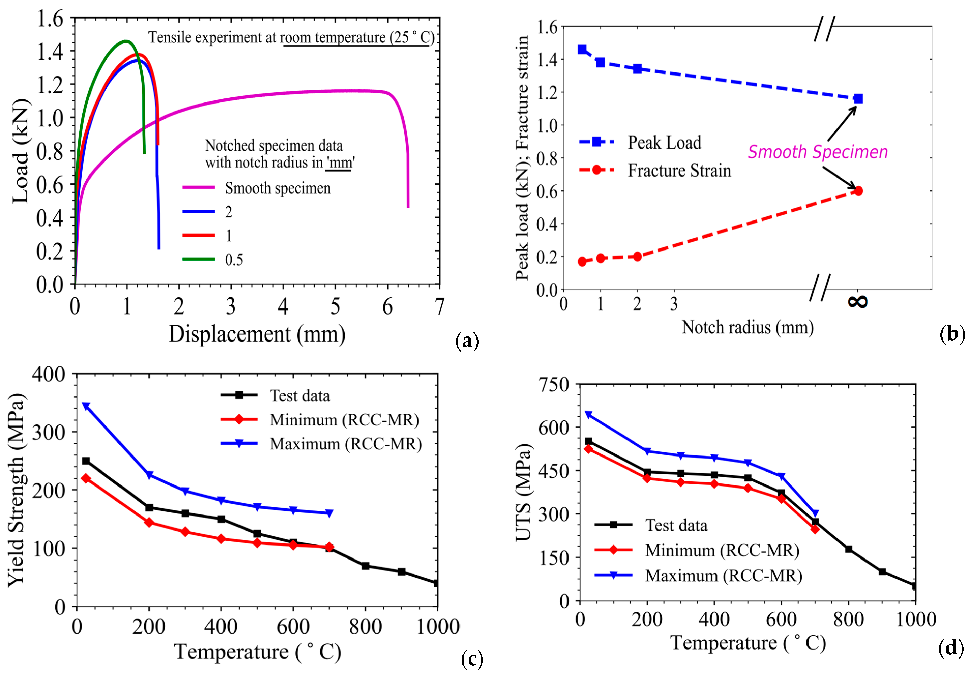
The notched tensile specimens (with different notch radii of 0.5, 1, and 2 mm) have been tested at 25 °C and the corresponding load-displacement data have been presented in Figure 2a. The notched specimens have been designed in such a way that the minimum cross-sectional areas (i.e., 1 × 2 mm²) of both smooth and notched type tensile specimens are kept the same. This shall help in studying the effect of stress triaxiality (which has been induced indirectly by changing the value of the notch radius) on fracture strain and the notch-strengthening behavior. As shown in Figure 2a, the hardening behavior and the peak load increase significantly for the notched specimens when compared to that of the smooth specimen, though the minimum cross-sectional areas of both types of specimens are the same. It can be explained on the basis of the development of a high-stress triaxial condition in the notched region of the notched specimens, which retards the onset and propagation of the plastic deformation process.

The details of the procedure for evaluation of stress triaxiality (which requires FE analysis) as a function of notch radius shall be discussed later. It is known that plastic yielding (based on von Mises criteria, also known as distortion energy theory) is independent of hydrostatic stress and hence, of stress triaxiality. The presence of higher values of the triaxial stress field (the lesser the notch radius) prevents plastic deformation for the same magnitude of applied remote tensile stress (and uniaxial load applied away from the notched region of the specimen), and hence, the notched specimens require more load to undergo similar extents of plastic deformation as that of the smooth tensile specimen. This is reflected in the load-displacement results of different types of specimens as presented in Figure 2a.

Moreover, the fracture displacement (and strain) also reduces with decreasing notch radius of the specimen and increasing stress triaxiality as presented in Figure 2a,b. The peak load-carrying capacity of the notched specimen also increases with decreasing notch radius, as presented in Figure 2a,b, and this phenomenon is also known as the notch-strengthening effect. However, it may be noted that the material true stress-strain curve, as used in material constitutive models in FE analysis (which uses von Mises criteria), is independent of stress triaxiality in the specimen, and hence, the notch strengthening is a geometrical phenomenon.

Another issue that arises in the evaluation process of fracture strain and stress triaxiality values in notched specimens is that these values are neither constant for a specimen (with a given geometry and notch radius) nor uniform across the minimum cross-sectional area, unlike that of a smooth tensile specimen, where the magnitude of stress triaxiality (defined as the ratio of hydrostatic stress to von Mises equivalent stress) is 1/3. These issues have been addressed in this work through the use of FE analysis, and the details shall be presented in the later sections.

The yield strength and UTS of SS316LN at different temperatures have been presented in Figure 2c,d. It may be noted that the yield strength decreases monotonically with an increase in temperature due to softening of the matrix of the material and easy movement of dislocations due to higher thermal activation. The decrease in yield strength and UTS from 25 to 200 °C is somewhat rapid, followed by a slow decrease in the magnitudes of the above properties in the temperature range of 200–600 °C. After 600 °C, the UTS decreases rapidly due to the onset of instability in the microstructure [27,28,29,30,31,32,33] of the material as discussed earlier.

The decrease in yield strength (YS) is not so rapid as compared to the change in UTS values, as YS signifies the onset of plastic deformation (or the process of initiation of yielding), and hence, the effect of microstructural instabilities becomes significant only at larger magnitudes of plastic deformations, and hence, it affects the UTS more. The mechanical properties (YS and UTS), as evaluated in this work, have also been compared with lower and upper-bound data of the same material, as presented in the French design and safety analysis code RCC-MR [3]. However, RCC-MR does not provide data up to 1000 °C as can be seen from Figure 2c,d. It can be observed that our data follows the trend of RCC-MR data for the whole temperature range, and these test data are also within the two statistical bounds of RCC-MR data. After evaluation of temperature-dependent mechanical properties and the true stress-strain curves for SS316LN, we have used the information to evaluate the parameters of material constitutive models, such as those of Johnson–Cook and Ramberg–Osgood. The process of evaluation of the parameters of these models, using conventional procedures, has some issues, which have been addressed in the subsequent sections.

4. Conventional Procedure and a New Algorithm for Evaluation of Parameters of Temperature and Strain-Rate-Dependent Material Constitutive Models

For the evaluation of plastic strain hardening, strain-rate hardening, and thermal softening parameters of SS316LN, the Johnson–Cook material model [4] has been used in this work. In this model, von Mises equivalent true stress ‘σ’ is expressed as a function of equivalent plastic strain ε_pl, true equivalent plastic strain rate $\dot{\epsilon }$, normalized temperature T* or T_norm as presented in Equation (1). The differential temperature (i.e., the difference between operating temperature T or T_ref) is normalized with respect to the differential value of melting temperature of the material T_m (w.r.t T_ref) as presented in Equation (2) to define the normalized parameter T*. The first term in Equation (1) represents the plastic strain hardening term, the second term refers to the strain-rate hardening term, and the last term corresponds to the thermal softening term.

$$\sigma =\left(A+B{\epsilon }_{\mathrm{pl}}^n\right)\left(1+C\ln \left\{{\displaystyle \frac{\dot{\epsilon }}{{\dot{\epsilon }}_{\mathrm{ref}}}}\right\}\right)\left(1-T_{\mathrm{norm}}^{\mathrm{m}}\right)$$

(1)

$$T_{\mathrm{norm}}\mathrm{or}T*=\left(T-T_{\mathrm{ref}}\right)/\left(T_{\mathrm{m}}-T_{\mathrm{ref}}\right)$$

(2)

In this work, the reference temperature is taken as 25 °C and hence, for room temperature tests, the Johnson–Cook material model can be expressed as given in Equation (3), where the last term of Equation (1) becomes unity.

$$\sigma =\left(A+B{\epsilon }_{\mathrm{pl}}^n\right)\left(1+C\ln \left\{{\displaystyle \frac{\dot{\epsilon }}{{\dot{\epsilon }}_{\mathrm{ref}}}}\right\}\right)$$

(3)

The issue of evaluation of flow stress (also known as true stress) as a function of cumulative plastic deformation, strain rate, and temperature and its presentation in a relevant coupled mathematical form (suitable for incorporation in material constitutive models in FE simulations) has been studied extensively in the literature [4,76,77,78].

However, the model proposed by Johnson and Cook [4] has unique advantages in its simplicity and ability to model the plastic strain hardening behavior of a wide class of materials ranging from carbon steel, low-alloy steel, copper, aluminum, stainless steel, magnesium, and other engineering materials. Later, the plastic strain hardening model was supplemented with a damage model [79] by taking into account the fracture characteristics of different types of materials when subjected to various magnitudes of strains, strain rates, temperatures, and hydrostatic pressures (also presented as stress triaxiality).

The model as presented in Equation (4) expresses equivalent plastic stain ${\overline{\epsilon }}_{\mathrm{D}}^{\mathrm{pl}}$ at damage (which is a critical value of equivalent plastic strain at which the onset of material degradation occurs and the material point subsequently loses its stress-carrying capability by reducing the strength in an exponential decay-type manner) as a function of stress triaxiality, strain rate, and normalized temperature.

$${\overline{\epsilon }}_{\mathrm{D}}^{\mathrm{pl}}=\left[d_1+d_{2}exp\left({-d}_3{\displaystyle \frac{p}{q}}\right)\right]\left[1+d_4\mathrm{*}ln\left({\displaystyle \frac{{\dot{\overline{\epsilon }}}_{\mathrm{pl}}}{{\dot{\epsilon }}_{\mathrm{r}\mathrm{e}\mathrm{f}}}}\right)\right]\left(1+d_5{T}^{*}\right)$$

(4)

where ${\mathit{d}}_1,{\mathit{d}}_2,{\mathit{d}}_3,{\mathit{d}}_4$ and ${\mathit{d}}_5$ are called the damage parameters of the Johnson–Cook model. The stress triaxiality ($\eta$) is defined as $p/q$ where $p$ and $q$ are the hydrostatic (mean) stress and von Mises equivalent stress values, respectively. Later, several modifications to the mathematical forms of the Johnson–Cook model have been carried out by various researchers [80,81]. Some of these expressions are presented here briefly. A modified form of the JC model was presented in Ref. [80] to model the material deformation behavior during the hot stamping process of B1500HS boron steel. This modification included a power law exponent $k$ in the strain-rate-dependent term (i.e., second bracket) and an additional coefficient $D$ in the temperature-dependent term (i.e., third bracket) as presented in Equation (5) below.

$$\sigma =\left(A+B{\epsilon }_{\mathrm{pl}}^n\right)\left[1+C{\left(\ln \left\{\dot{\epsilon }/{\dot{\epsilon }}_{\mathrm{ref}}\right\}\right)}^{\mathrm{k}}\right]\left[1-D{\left(T_{\mathrm{norm}}\right)}^{\mathrm{m}}\right]$$

(5)

Later, Wang et al. [81] modified the plastic strain-dependent term (i.e., the term in the first bracket) of Equation (1), and they instead used a quadratic polynomial expression instead of the power law as presented in Equation (6). In addition, the strain-rate and temperature-dependent terms were coupled together and expressed through an exponential function as presented in the third term of Equation (6).

$$\sigma =\left(A_1+B_1{\epsilon }_{\mathrm{pl}}+B_2{\epsilon }_{\mathrm{pl}}^2\right)\left[1+C\ln \left\{\dot{\epsilon }/{\dot{\epsilon }}_{\mathrm{ref}}\right\}\right]\exp \left[\left({\lambda }_1+{\lambda }_2\ln \left\{\dot{\epsilon }/{\dot{\epsilon }}_{\mathrm{ref}}\right\}\right)\left(T-T_{\mathrm{ref}}\right)\right]$$

(6)

Zou et al. [82] further modified the plastic strain-dependent term of the true stress through a cubic polynomial as presented in Equation (7), keeping the other two terms similar to those of Ref. [81].

$$\sigma =\left(A_1+B_1{\epsilon }_{\mathrm{pl}}+B_2{\epsilon }_{\mathrm{pl}}^2+B_3{\epsilon }_{\mathrm{pl}}^3\right)\left[1+C\ln \left\{\dot{\epsilon }/{\dot{\epsilon }}_{\mathrm{ref}}\right\}\right]\exp \left[\left({\lambda }_1+{\lambda }_2\ln \left\{\dot{\epsilon }/{\dot{\epsilon }}_{\mathrm{ref}}\right\}\right)\left(T-T_{\mathrm{ref}}\right)\right]$$

(7)

The method of identification of parameters of the Johnson–Cook material model as presented through Equations (1) and (4) is very challenging as it involves several types of specimen design for the tests, which include smooth as well as notched tensile specimens, high strain-rate tests, high-temperature tests, etc.

Moreover, the procedure for evaluation of stress triaxiality values for different types of notched tensile specimens requires the use of a complex analysis procedure, which is not trivial for an experimentalist, and these also cannot be directly evaluated from experimental measurement as conducted while evaluating mechanical properties such as YS, UTS, and ductility, etc. Several works have been reported in the literature [81,82,83,84,85,86,87,88] regarding the identification of parameters of the Johnson–Cook material model. This damage model has also been used in Ref. [85] to evaluate the machinability characteristics of the materials.

The model parameters have been evaluated using an optimization approach involving the fireworks algorithm in Ref. [87]. It can be seen that the procedure for identification of Johnson–Cook model parameters, especially the damage parameters (i.e., d₁ to d₅), is complex. It needs a thorough understanding of the model as regards its applicability in simulating material deformation behavior at different temperatures and strain rates. In this work, the conventional method for identification of the parameters shall be presented first.

The difficulty of the process of identification of the parameters (as evaluated using the conventional procedure) shall be highlighted first by comparing the results of the FE simulation with a wide range of experimental data, and a new procedure shall be presented later, which is based on minimization of error in simulation of load-displacement behavior of different types of specimens (when compared with experimental data).

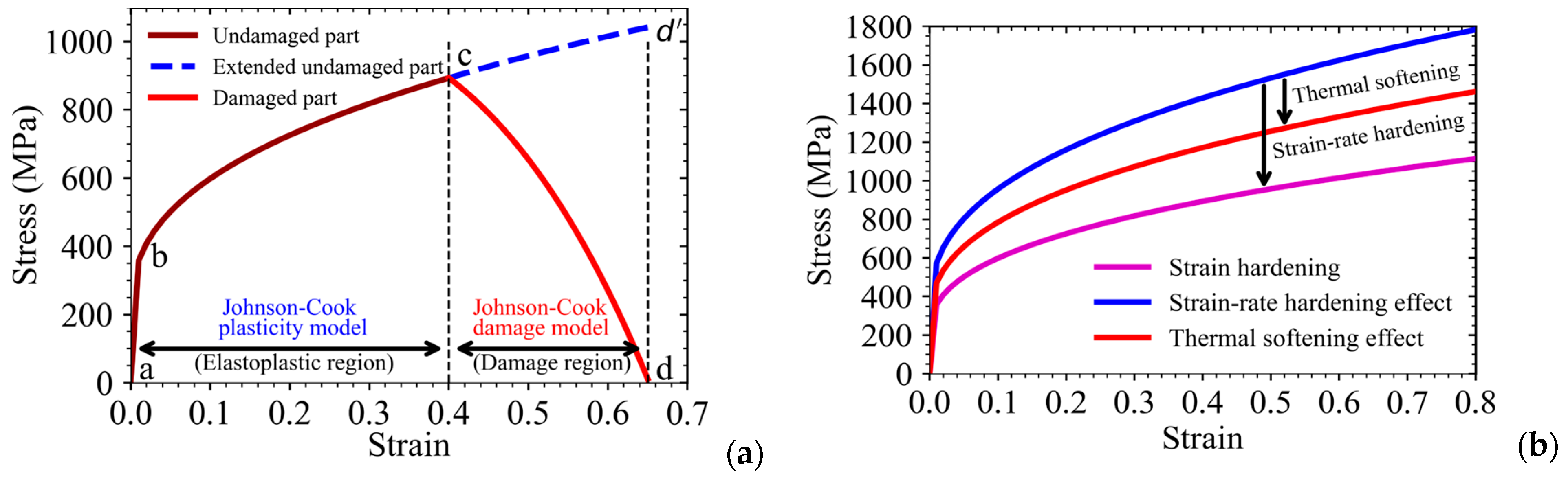
Before proceeding with the discussion regarding the evaluation of parameters of the Johnson–Cook material model, a schematic explanation of the material hardening and softening responses of the material (as presented by the above model) is presented in Figure 3. This figure represents the variation of true stress in the material point as a function of cumulative equivalent plastic strain. The curve as presented in Figure 3a has been divided into two parts, i.e., the plastic hardening part represented by the Johnson–Cook plasticity model (Equation (1)) and the damage region represented by the Johnson–Cook damage model (Equation (4)). Once the critical value of equivalent plastic strain for damage as presented in Equation (4) is reached in the material point during the ongoing deformation, damage initiation and propagation start, which simulates the void nucleation, growth, and coalescence in ductile materials.

The material point loses its stress-carrying capacity with further plastic straining, which leads to a reduction in the true stress of the material as presented in Figure 3a. Once the true stress becomes zero, the material point loses the complete stress-carrying capacity, and hence, it becomes a microscopic crack in the material volume. This way, the damage model helps simulate crack initiation and growth, not only in the tensile specimens but also in the fracture specimens and cracked components. Hence, the coupled plasticity and damage model as presented by Johnson and Cook is very useful to simulate crack propagation under a given loading condition and hence, to carry out structural integrity analysis during postulated severe accident scenarios.

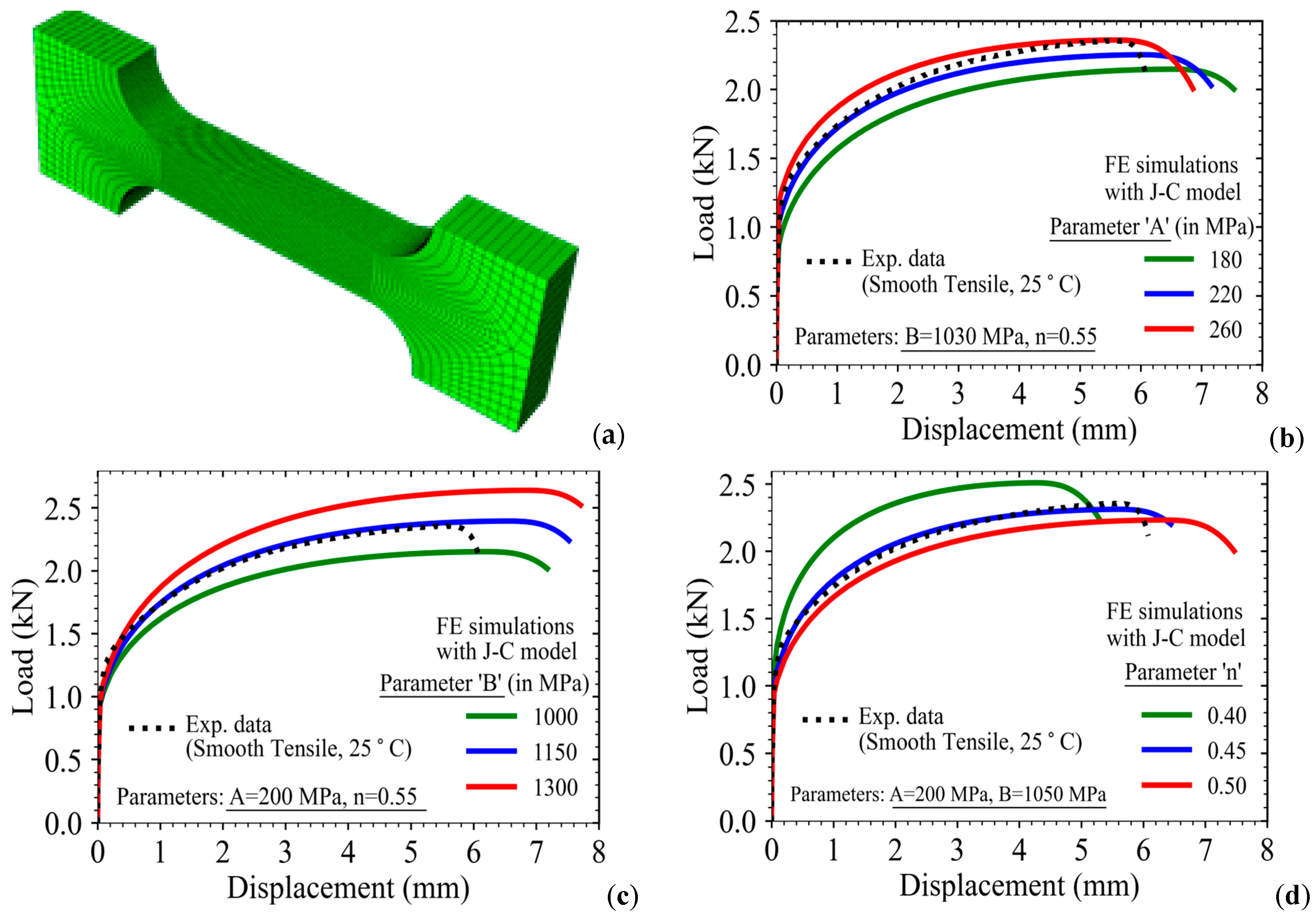
The strain rate hardening and thermal softening behavior of the material (as presented through the Johnson–Cook model) have been presented schematically in Figure 3b. This model, when coupled with the damage model, as presented in Figure 3a, constitutes the complete Johnson–Cook material model. There are three parameters of the Johnson–Cook plasticity model, i.e., A, B, and ‘n’. The third parameter represents the conventional plastic strain hardening coefficient of the material. The effect of these three parameters on the material’s true stress-strain curve is shown in Figure 4.

When the parameter ‘A’ is increased (keeping the other two parameters the same), it shifts the whole true stress-strain curve almost in a parallel manner with respect to the initial curve (Figure 4a). The parameter ‘B’ controls the shape or nature of the change in slope of the true stress-strain curve (Figure 4b). A higher value of ‘B’ represents a steeper slope of the curve. The third parameter, ‘n’, represents strain hardening behavior (Figure 4c). The bilinear stress-strain curve (i.e., linear plastic hardening), which is widely used in the design of components (due to its simplicity) and also in literature, is represented by ‘n = 1’, i.e., a straight line.

The zero value of strain hardening represents elastic-perfectly plastic material behavior. The effect of these individual parameters provides insight into the process of evaluation of these parameters from the experimentally obtained material stress-strain data and compares the relative plastic hardening response of different types of materials and alloys. The effect of these three parameters, however, becomes clearer once these are used in FE simulations of both smooth and notched type tensile specimens as presented in Figure 5 and Figure 6, respectively.

Finite element analysis of the tensile specimens has been carried out using the commercial program ‘Abaqus’. For the analysis of each specimen, 3D 8-noded solid brick-type trilinear elements have been used. The minimum size of elements (i.e., mesh size) has been taken to be 0.1 mm. Initially, a mesh convergence study was carried out in order to select the least size of elements to be used in FE analysis so that the results become independent of mesh size. For example, the smooth tensile specimen has been modeled using 3D solid brick-type elements as shown in Figure 5a, and the total number of 3D solid elements stands at approximately 87,000 (the minimum mesh size is 0.1 in each direction at the minimum cross-section of the specimen). The geometry of these specimens is the same as those used in earlier experiments, and the geometrical details are shown in Figure 1a. The Johnson–Cook material model as implemented in the code ‘Abaqus’ has been used for the analysis.

The specimen has been fixed at one end along its length, and a displacement-controlled loading has been applied at the other end of the specimen as shown in Figure 1a. The load-displacement data as obtained from FE analysis for various values of parameters ‘A’, ‘B’, and ‘n’ are shown in Figure 5b–d. It may be noted that while varying one parameter at a time, the other two parameters are kept unchanged. Figure 5b shows the effect of parameter ‘A’ on the load-displacement response of the smooth tensile specimen.

This curve shifts in a parallel fashion with an increase in the value of ‘A’, whereas the necking process initiates early. This early onset of necking could not be observed earlier in Figure 4a as it did not model the associated geometrical nonlinearity phenomenon, which is prevalent in components subjected to predominant tensile loading. Hence, the study of component-level load-displacement behavior is more important from the point of view of analysis with the Johnson–Cook material model and the corresponding process of parameter evaluation while using combined experimental and FE analysis approaches.

The effect of parameter ‘B’ is shown in Figure 5b. It may be noted that the slope of the load-displacement curve increases with an increase in this parameter, whereas the onset of necking (as indicated by the point of load drop) is delayed. Hence, this parameter affects both the strength and ductility of the smooth tensile specimen. The effect of parameter ‘n’ on the load-displacement curve of the smooth tensile specimen is shown in Figure 5c, where it is seen to affect both the strain-hardening behavior and the ductility. The onset of necking in the tensile specimen is delayed by increasing the value of parameter ‘n’.

The effect of these 3 parameters on the load-displacement curve of the notched tensile specimen is shown in Figure 6. The 3D FE mesh of a typical notched specimen is shown in Figure 6a. Similar effects of the parameters on the load-displacement curve as observed for smooth specimens are also seen here, except that the load drop after reaching maximum load is not sudden in these specimens. If one looks at experimental data as presented in Figure 2a for the notched tensile specimens, the load drop occurs relatively fast after reaching maximum load.

This discrepancy between experimental and FE analysis results can be explained from the context of the development of damage in the notched regions of the notched tensile specimens. In these parametric study examples presented in Figure 5 and Figure 6, the effect of material damage as represented by the Johnson–Cook damage model (i.e., Equation (4)) has not been considered, and hence, the plasticity model alone is not able to simulate the experimentally observed nature of load drop in notched tensile specimens. In smooth specimens, the damaging effect is not reflected in the load-displacement curve predominantly as the initiation of necking due to geometrical nonlinearity reduces the load-carrying capability of the specimen drastically due to a sudden change in the load-carrying cross-section (i.e., after the onset of necking in the specimen).

In the notched specimen, we have a notched region already, which delays yielding and subsequent plastic deformation due to the presence of a triaxial state of stress. In the experiment, the load drop in the specimen occurs due to the development of damage in the notched region, and the higher stress triaxiality accelerates the process of damage accumulation, leading to an early drop of load and hence, a fracture of the specimen. As mentioned earlier, coupling both the plastic hardening and damage models can address this issue, and this coupled approach will be presented later in this paper. One further observation can be noted from this analysis of load-displacement curves of notched tensile specimens, i.e., the parameters ‘A’ and ‘n’ do not affect the regions beyond the peak loads of the specimens (Figure 6b,d), unlike that of parameter ‘B’ as presented in Figure 6c.

In order to evaluate the parameters ‘A’, ‘B’, and ‘n’ of the Johnson–Cook material model of SS316LN, the true stress-strain curve as presented in Figure 1e for the room temperature test has been used. For room temperature tests (T = T_ref) at quasi-static loading conditions (i.e., the strain rate of the experiment is the same as the reference strain rate), the second and third terms of Equation (1) become unity. Hence, by fitting the first term of Equation (1) with the above test data, the parameters have been evaluated as A = 200 MPa, B = 1160 MPa, and n = 0.59, respectively. These parameters have been used in the FE simulation of the split Hopkinson pressure bar test (i.e., high strain rate test) to evaluate the strain-rate-dependent parameter ‘C’ of the Johnson–Cook material model as discussed below.

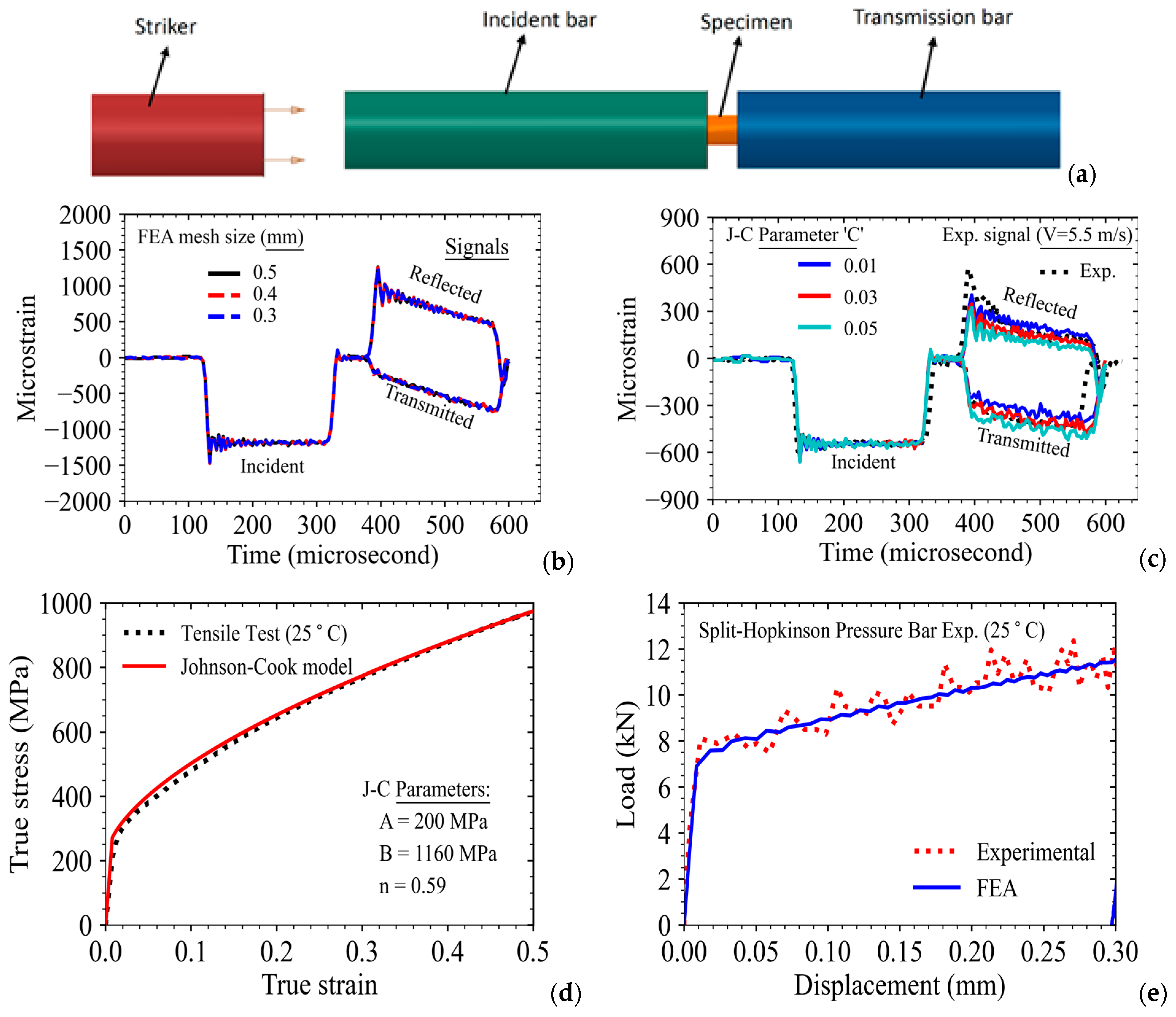
The split Hopkinson pressure bar (SHPB) test is widely used to carry out high-strain rate tests, and a schematic view of the test setup is presented in Figure 7a. The test setup consists of a striker, an incident bar, and one transmission bar. The cylindrical specimen (5 mm diameter and 5 mm length) is sandwiched between the incident and the transmitted bars as shown in Figure 7a. The striker bar is fired at a particular velocity using a gas gun, and the velocity of the striker is controlled through pressure in the gas gun chamber.

Upon release from the gas gun, the striker hits the incident bar, where a traveling elastic strain pulse is generated, this pulse travels along the length of the incident bar, and upon reaching the specimen interface, a part of the strain wave is reflected, and the rest is transmitted across the specimen to the transmission bar. The plastic deformation of the cylindrical specimen affects the nature of the reflected and the transmitted waves, whereas the nature of the incident pulse is dependent upon the striker velocity and its length.

The incident, reflected, and transmitted strain wave signals are captured through two strain gauges located at the center of the incident and transmission bars using appropriate signal conditioning electronics. The details of the test setup and experimental procedure can be found in Ref. [88]. All the bars have been designed in such a way that they remain elastic during the high strain rate experiment so that the strain wave is of elastic nature, and hence, the standard expressions for evaluation of strain, strain rate, and stresses in the specimen can be utilized while evaluating the data from the strain wave signals as shown in Equation (8).

$$\dot{{\epsilon }_{\mathrm{s}}}={\displaystyle \frac{2C_{\mathrm{o}}{\epsilon }_{\mathrm{r}}}{L_{\mathrm{s}}}};{\epsilon }_{\mathrm{s}}={\displaystyle \frac{2C_{\mathrm{o}}}{L_{\mathrm{s}}}}{\int }_0^{\mathrm{t}}{\epsilon }_{\mathrm{r}}dt;{\sigma }_{\mathrm{s}}={\displaystyle \frac{AE{\epsilon }_{\mathrm{t}}}{A_{\mathrm{s}}}}$$

(8)

In this equation, $\dot{{\epsilon }_{\mathrm{s}},}$ ${\epsilon }_{\mathrm{s}},$ and ${\sigma }_{\mathrm{s}}$ represent stain-rate, strain, and stress in the specimen, ${\epsilon }_{\mathrm{r}}\mathrm{and}{\epsilon }_{\mathrm{t}}$ are the stain signals of the reflected and transmitted waves (these signals vary with time during the test and are functions of time), $C_{\mathrm{o}}$ is the velocity of the traveling wave in the bars, $A\mathrm{a}\mathrm{n}\mathrm{d}E$ are cross-sectional area and Young’s modulus of elasticity of both the bars (these are same for both incident and transmission bars), $A_{\mathrm{s}}\mathrm{a}\mathrm{n}\mathrm{d}{L}_{\mathrm{s}}$ are cross-sectional area and length of the cylindrical specimen.

In this work, the velocity of the striker bar is kept at 5.5 m/s, which corresponds to 1 bar pressure in the firing chamber of the gas gun. The average strain rate corresponds to 500 per second for this velocity of impact. However, it may be noted that the strain rates vary during the SHPB test, and it is a major limitation while evaluating the strain-rate-dependent parameter ‘C’ of the Johnson–Cook material model from the test data. The conventional procedure involves evaluation of the true stress-strain curve from the reflected and transmitted strain signals using standard expressions as presented in Equation (8) and fitting of the parameter ‘C’ from this average strain-rate dependent data.

It shall be clearer if one looks into the data presented in Figure 7b, which correspond to a typical incident, transmitted, and reflected strain signals as obtained from a typical SHPB test with a cylindrical specimen. From Equation (8), the strain rate is directly proportional to the reflected strain wave, and its magnitude continuously decreases with time during the test. This signifies the varying strain rate experienced by the specimen in the SHPB test. This is usually ignored in the conventional procedure as followed in literature while evaluating the parameters from the data of SHPB tests. This issue has been addressed in this work by resorting to FE analysis of the SHPB test setup to optimize the parameter ‘C’ instead of fitting Equation (1) to the average stress-strain curve obtained from SHPB tests. The details are discussed in the following paragraph.

The specimen, along with the incident and transmission bars, has been modeled using 3D finite elements, and contact conditions between the specimens and the bars have been modeled. The left end of the incident bar has been provided with a velocity of 5.5 m/s. Upon impact of the striker bar with the incident bar, the strain signals from the centers of the incident and the transmission bars have been evaluated from FE analysis, and these are plotted in Figure 7b. For elastic bars, only values of Young’s modulus ‘E’ and Poisson’s ratio ‘ν’ are required, and these are taken as 210 GPa and 0.3, respectively, which correspond to data of the material of the bars used in the test setup.

Before presenting the results of the analysis, a mesh convergence study has been carried out using different mesh sizes in the specimen ranging from 0.3 to 0.5 mm. It may be observed that the mesh used in the analysis is sufficiently fine and the results of the analysis are independent of the FE mesh size. For this analysis, the Johnson–Cook material plasticity model has been used, and these parameters are taken as follows, i.e., A = 200 MPa, B = 1160 MPa, and n = 0.59. The remaining strain-rate-dependent parameter ‘C’ has been used as a parameter in the FE analysis of the SHPB test setup. The results of the FE analysis with different values of ‘C’ ranging from 0.01 to 0.03 are plotted in Figure 7c along with the experimental data. It may be observed that the strain wave signals as obtained from FE analysis match almost closely with experimental data for ‘C = 0.03’.

This value of the parameter ‘C’ better represents the experimentally observed plastic deformation behavior of the specimen at higher rates of loading, and hence, it represents the actual parameter of the Johnson–Cook material model for SS316LN. This procedure has advantages over the conventional procedure as it takes care of the varying strain rate in the SHPB model by modeling the strain signals directly instead of using stress-strain data (corresponding to an average strain rate) for evaluating parameter ‘C’ as reported in the conventional procedure.

The accuracy of the plasticity parameters of the Johnson–Cook model as evaluated for the material SS316LN has been verified by comparing the stress-strain curves as obtained from quasi-static experiments with those predicted by the model (using Equation (1)), and the results are presented in Figure 7d. Similarly, the load-displacement response for the cylindrical specimen loaded with 5 m/s velocity in the SHPB setup as predicted by FE simulation has been compared with the corresponding experimental data in Figure 7e. The FE results with the Johnson–Cook model show a close match with the corresponding experimental data. Hence, the method developed and adopted in this work is more elegant and versatile when compared to the conventional procedure followed in the literature.

For evaluation of the parameter ‘m’ in the third term of Equation (1), high-temperature tensile tests have been carried out, and the true stress-strain data have been presented earlier in Figure 1d. As the parameters of the first and second terms of the Johnson–Cook plasticity model have been evaluated already following the procedure described in earlier sub-sections, this sub-section presents the method of evaluation of the temperature-dependent parameter ‘m’ using both the conventional procedure (as reported in the literature) and the new procedure developed in this work. The first and second terms in Equation (1) have been evaluated using A = 200 MPa, B = 1160 MPa, n = 0.59, and C = 0.03.

The true stress-strain data at various test temperatures have been normalized with the plastic strain hardening and strain-rate hardening terms, which are also functions of cumulative plastic strain in the material. These tests have been conducted under quasi-static strain conditions. The strain rate of the tests corresponds to the reference strain rate of the Johnson–Cook material model, and hence, the second term of Equation (1) becomes unity.

The normalized true stress has been plotted as open circles in Figure 8a for each test temperature. One can see the extent of scatter in the data for a given temperature as the conventional method uses all the data of the true stress-strain curve at various temperatures directly in Equation (1) to evaluate the parameter ‘m’. This is exactly the reason why this conventional procedure may introduce errors in the evaluation of parameter ‘m’ of the Johnson–Cook model.

This shall be clearer once we compare the results of the FE analysis of high-temperature tensile tests with those of experiments using the parameter ‘m’ (estimated using the conventional method). The value of ‘m’ has been estimated to be ‘1.02’ as can be seen from the slope of the best-fit straight line in Figure 8a. The load-displacement results of the FE simulation, as obtained from the analysis of smooth tensile specimens at different temperatures, are presented in Figure 8b–d.

It can be noted that the results predicted by the FE model do not compare well with the experimental data for different test temperatures. The value of parameter ‘m’ as estimated by the conventional method seems to be lower compared to the actual material property. The lower value of ‘m’ corresponds to more thermal softening, and hence, all the FE predicted load-displacement curves are found to be lower when compared to the actual experimental data (at all the temperatures) as presented in Figure 8b–d.

The conventional method is found to be inadequate for evaluation of the temperature-dependent parameter ‘m, and hence, a new optimization procedure has been adopted to estimate this parameter more accurately. In the new procedure, the results of FE analysis have been utilized along with the experimental data in order to optimize the parameter ‘m’. This results in a parameter that corresponds to the minimum error between load-displacement data as obtained from FE analysis and experiment for all tests at different temperatures.

The absolute difference of area between the load-displacement curves (up to the displacement corresponding to rapid load drop in the experiment) as obtained from the experiment and FE analysis (e.g., Figure 8b–d) has been utilized as an objective function with a variable parameter ‘m’. A range of values of ‘m’ has been utilized in FE analysis of high-temperature tensile tests, keeping other parameters (i.e., A, B, n, and C) the same as determined earlier. In this work, the values of ‘m’ have been varied from 1 to 1.4, which also covers the initial estimate of ‘m’ (i.e., 1.02) in the conventional method. The magnitudes of error (i.e., the absolute difference of area) between load-displacement curves as obtained from FE analysis and those of the experiment are presented as a function of parameter ‘m’ in

Table 3. Variation of absolute difference in the area of load-displacement curves of experiment and FE analysis for various values of parameter ‘m’.

Johnson–Cook Parameter ‘m’	Area_Test (kN-mm)	Area_FEA (kN-mm)	Error = Absolute Difference (kN-mm)
1	9.27	8.8	0.47
1.1	9.27	9.15	0.12
1.2	9.27	9.45	0.18
1.3	9.27	9.71	0.44
1.4	9.27	9.94	0.67

.

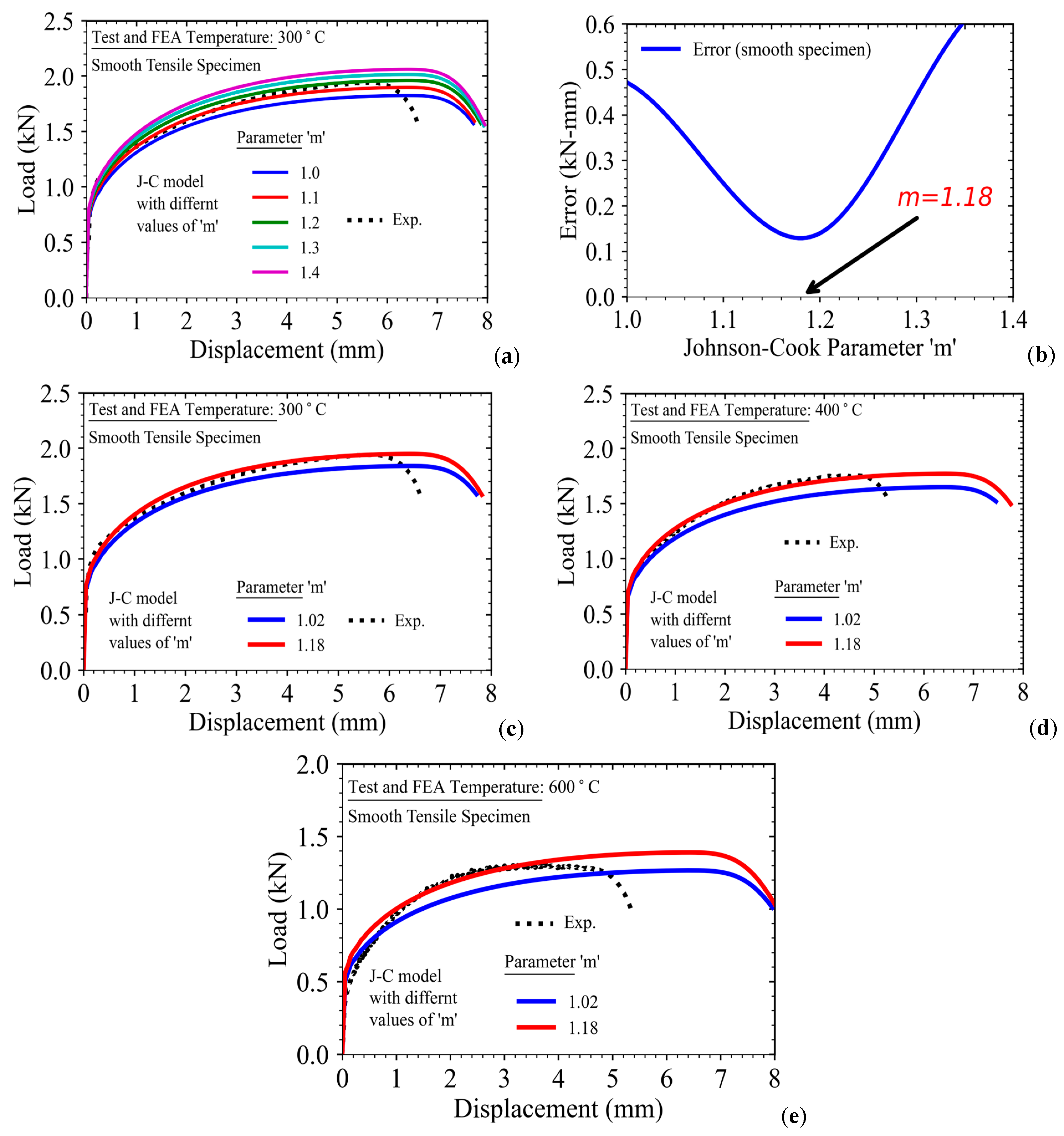
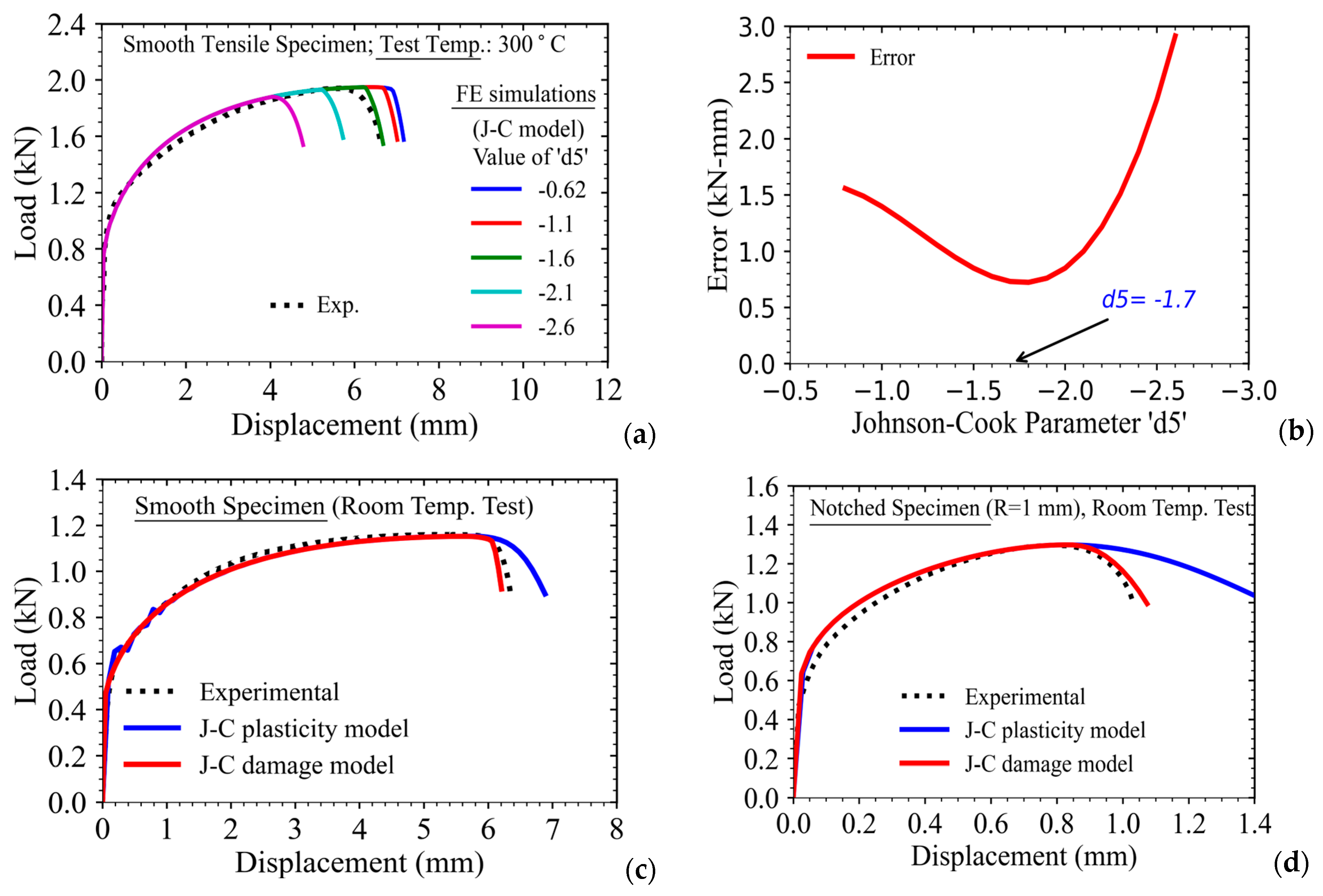
A typical load-displacement data as obtained from testing of tensile specimens at 300 °C is presented in Figure 9a. The results of the FE analysis with the Johnson–Cook plasticity model have also been plotted in Figure 9a along with the experimental data by varying the parameter ‘m’ while keeping all other parameters unchanged. It can be observed from Figure 9a that the load-displacement curves as predicted by the FE model tend to shift higher almost in a parallel manner when the value of ‘m’ is increased.

This means a lower value of ‘m’ represents more thermal softening and vice versa. The absolute difference in the area between load-displacement curves as obtained from FE analysis and experiment (up to the point of load drop in the test) has been plotted as a function of parameter ‘m’ in Figure 9b. As can be seen from this data, the error initially decreases with an increase in ‘m’ and then increases. The error is minimum, corresponding to the value of ‘m = 1.18’.

Hence, this value has been taken as the optimum value of ‘m’ corresponding to the minimum error between the results of the FE simulation and the experiment. In order to verify the new methodology adopted in this work, the results of the FE simulation with ‘m = 1.18’ have been compared with experimental data for different test temperatures, and the results are presented in Figure 9c–e. The FE results with ‘m = 1.02’ are also presented along with the results evaluated with the optimized parameter ‘m = 1.02’.

It can be observed that the results of the FE analysis compare very well with experimental data for all the temperatures, whereas the results of the simulation with ‘m = 1.02’ (as estimated using the conventional procedure) are clearly inadequate in representing the experimentally observed material deformation behavior at different temperatures.

One more important aspect can be noted from the results presented in Figure 9b–e. It may be noted that the point of load drop in the FE simulation result of the specimen load-displacement data does not match well with the point of experimentally observed load drop. This is because the point of load drop corresponds to the development of damage in the specimen due to void coalescence phenomena.

In this plasticity model (Equation (1)), we are only modeling plastic strain hardening, strain-rate hardening, and thermal softening effects. The material damage (i.e., its onset and propagation) is modeled through the Johnson–Cook damage model as presented in Equation (4), and these aspects shall be taken care of in the subsequent sections of this paper. With the inclusion of both the damage and plasticity models, it shall be possible to model not only the overall load-displacement behavior but also the point of load drop as observed in the experiments at all the test temperatures. These results have been presented in the subsequent sections of this paper.

5. A New Optimization Technique for Evaluation of Plastic Hardening Parameters of the Ramberg–Osgood Model

As discussed earlier, the Ramberg–Osgood plastic hardening model [89] is used in FE simulations, in analytical solutions of elastic-plastic crack problems, and in the evaluation of crack-tip loading parameters of different types of specimens and components (with initial cracks) while employing the concept of elastic-plastic fracture mechanics for integrity analysis of industrial components. In particular, the Ramberg–Osgood parameters $n_{\mathrm{RO}}$ and ‘α’ are used in the closed-form expressions for the estimation of fracture or crack-tip loading parameters (such as J-integral, limit load, crack-tip stress, and strain fields in elastic-plastic materials, crack mouth opening displacement, load-line displacement, etc.) in the EPRI handbooks [74,75]. These parameters have been evaluated for nuclear-grade carbon steel from extensive experimental data, and the results are presented in Ref. [90]. The Ramberg–Osgood material model can be expressed through Equation (9).

$$\left(\epsilon /{\epsilon }_0\right)=\left(\sigma /{\sigma }_0\right)+\alpha {\left(\sigma /{\sigma }_0\right)}^{n_{\mathrm{RO}}}$$

(9)

In Equation (9), α (strain coefficient) and $n_{\mathrm{RO}}$ (strain hardening exponent) are material constants (note the use of the subscript ‘RO’ to denote the strain hardening coefficient in the Ramberg–Osgood model, whereas the symbol ‘n’ is used for the strain hardening coefficient in the Johnson–Cook model). ${\sigma }_0$ and ${\epsilon }_0$ are stress and strain values at the yield point of the material. Using the decomposition of strain into elastic and plastic components $\left(\mathrm{i}.\mathrm{e}.,\epsilon ={\epsilon }^{\mathrm{el}}+{\epsilon }^{\mathrm{pl}}\right)$ and noting that ${\epsilon }^{\mathrm{el}}=\sigma /E$ (where $E$ is Young’s modulus of elasticity of the material), the relationship between plastic strain (${\epsilon }^{\mathrm{pl}}$) and true stress ($\sigma$) can be rewritten as

$$\left({\epsilon }^{\mathrm{pl}}/{\epsilon }_0\right)=\alpha {\left(\sigma /{\sigma }_0\right)}^{n_{\mathrm{RO}}}$$

(10)

This strain hardening exponent paramegers $n_{\mathrm{RO}}$ for the Ramberg–Osgood stress-strain relationship is always greater than unity as the exponent is over true stress ‘σ’, i.e., true strain is represented as a function of true stress with a power law type equation, not vice versa. It may be noted that for the Johnson–Cook plasticity model, the strain hardening exponent is the inverse of the corresponding exponent of the Ramberg–Osgood model.

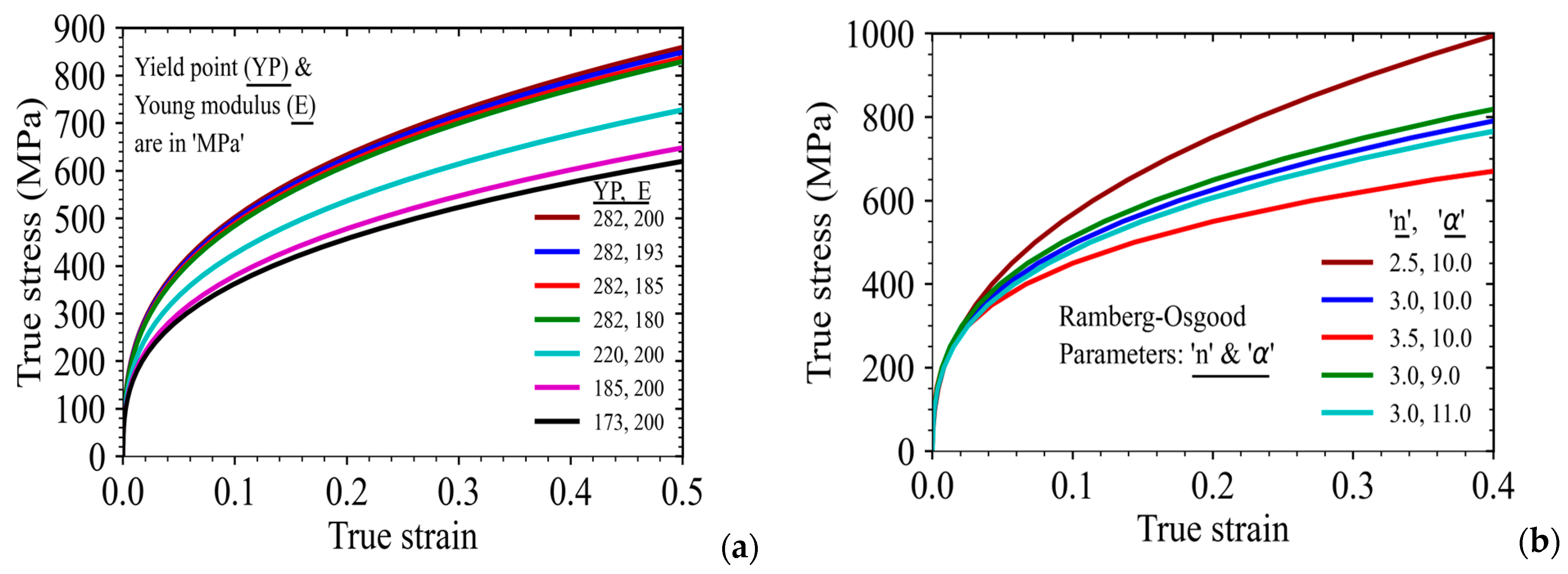
The effects of yield point strength (YP), Young’s modulus of elasticity (E) of the material, as well as those of Ramberg–Osgood parameters, $n_{\mathrm{RO}}$ and ‘α’ on the material’s true stress-strain curve have been shown in Figure 10. It can be observed that for a given value of yield strength, the stress-strain curve shifts upwards (however, very insignificantly) by increasing the values of ‘E’.

Hence, the variation in the value of ‘E’ does not have much effect on the plastic strain hardening behavior of the material when its values are varied between 180 and 200 GPa (Figure 10a). On the other hand, the parameter ‘YP’ has a very strong effect on the true stress-strain curve of the material as represented through the Ramberg–Osgood model. The stress-strain curve shifts upward significantly when the value of ‘YP’ is increased from 173 to 200 MPa, keeping the value of ‘E’ as 200 GPa.

Similarly, the effect of paramegers $n_{\mathrm{RO}}$ and ‘α’ on the material stress-strain curve is presented in Figure 10b. It may be noted that the parameter ‘α’ does not have much effect on the stress-strain curve when varied in the range of 9 to 11, whereas the strain hardening parameter has a significant effect when varied in the range of 2 to 3. A higher value of the strain hardening parameter (in the Ramberg–Osgood model) represents lesser strain hardening and vice versa. For elastic materials, this parameter is ‘1’ and for elastic-perfectly plastic material, this parameter tends to ‘∞’. This parametric study helps us in accurately identifying the parameters of the Ramberg–Osgood model from the test data.

In this work, a new procedure has been developed in order to evaluate the parameters of the Ramberg–Osgood plasticity model for SS316LN at different test temperatures. The method uses combined FE analysis and experimental data of smooth as well as notched tensile specimens to evaluate the error as a function of Ramberg–Osgood material parameters ‘n’ anf ‘α’, and the error has been minimized in order to evaluate the optimized parameters for the material at different temperatures.

The load-displacement data obtained from the tests of smooth and notched tensile specimens at room temperature are presented in Figure 11a. Four different notched specimens with notch radii of 0.5, 1.25, 2.5, and 5 mm have been used in the tests. It can be observed that the peak load of the notched tensile specimen increases with decreasing notch radius of the specimens as expected from earlier discussion, and these are significantly higher compared to the maximum load-carrying capacity of the smooth specimen due to the notch-strengthening effect.

However, the displacement at fracture reduces with a decrease in notch radius. This is due to the increase in stress triaxiality in the specimens, which accelerates the process of accumulation of damage in the notched region of the specimens. In order to develop a unique combination of Ramberg–Osgood material parameters ‘n’ and ‘α’, which is valid for both smooth and notched specimens, a new procedure has been developed here.

This is based on the minimization of error between load-displacement data as predicted by FE simulation and those of the experiment of smooth as well as notched specimens. The error is expressed in terms of the absolute difference in the area between the two curves as shown in Figure 10b for a typical notched tensile specimen. The absolute difference in the area has later been normalized with the gauge volume of the specimens in order to account for the difference in the volumes of the plastically deformed regions.

It may be noted that the plastic deformation is mainly confined to the notched region in the case of the notched specimen, whereas it is spread over the larger volume (i.e., the whole gauge length region) for the smooth specimen. The normalized error has been summed for all the specimens (smooth as well as notched, with different notch radii), and these have been plotted as a function of ‘$n_{\mathrm{RO}}$’ for a given value of ‘α’ in Figure 11c. From this figure, the value of ‘n’ corresponding to the minimum value of error has been found. A similar exercise has been carried out for other values of ‘α’, and a combination of parameters ‘n’ and ‘α’ corresponding to the minimum error has been presented in Figure 11d.

The optimization procedure followed in this work is a two-step process, as there are two parameters that are being optimized here. For all the combinations of parameters presented in Figure 11d, the error again has been plotted, and the minimum has been found to be for ‘n = 2.72, α = 10’ as presented in Figure 11e. These optimized parameters correspond to room temperature (i.e., 25 °C) test data.

Similarly, the procedure is repeated for a test temperature of 650 °C and the optimized values of the parameters have been found to be ‘$n_{\mathrm{RO}}$=2.67, α=8.62’ as shown in Figure 11f. It may be noted that the strain hardening exponent of the Ramberg–Osgood model is sensitive to temperature, as these represent the plastic strain hardening behavior of the material at different temperatures.

For evaluation of Ramberg–Osgood parameters at other temperatures in the 25–650 °C, the data points of stress-strain data from the RCC-MR code [3] for the material SS316LN have been used. It may be noted that RCC-MR provides data points only up to 1.5% plastic strain, whereas the fracture strain can be as high as 0.4 to 0.6. However, the values of the plastic hardening parameter of the Ramberg–Osgood model are mainly dictated by the initial data.

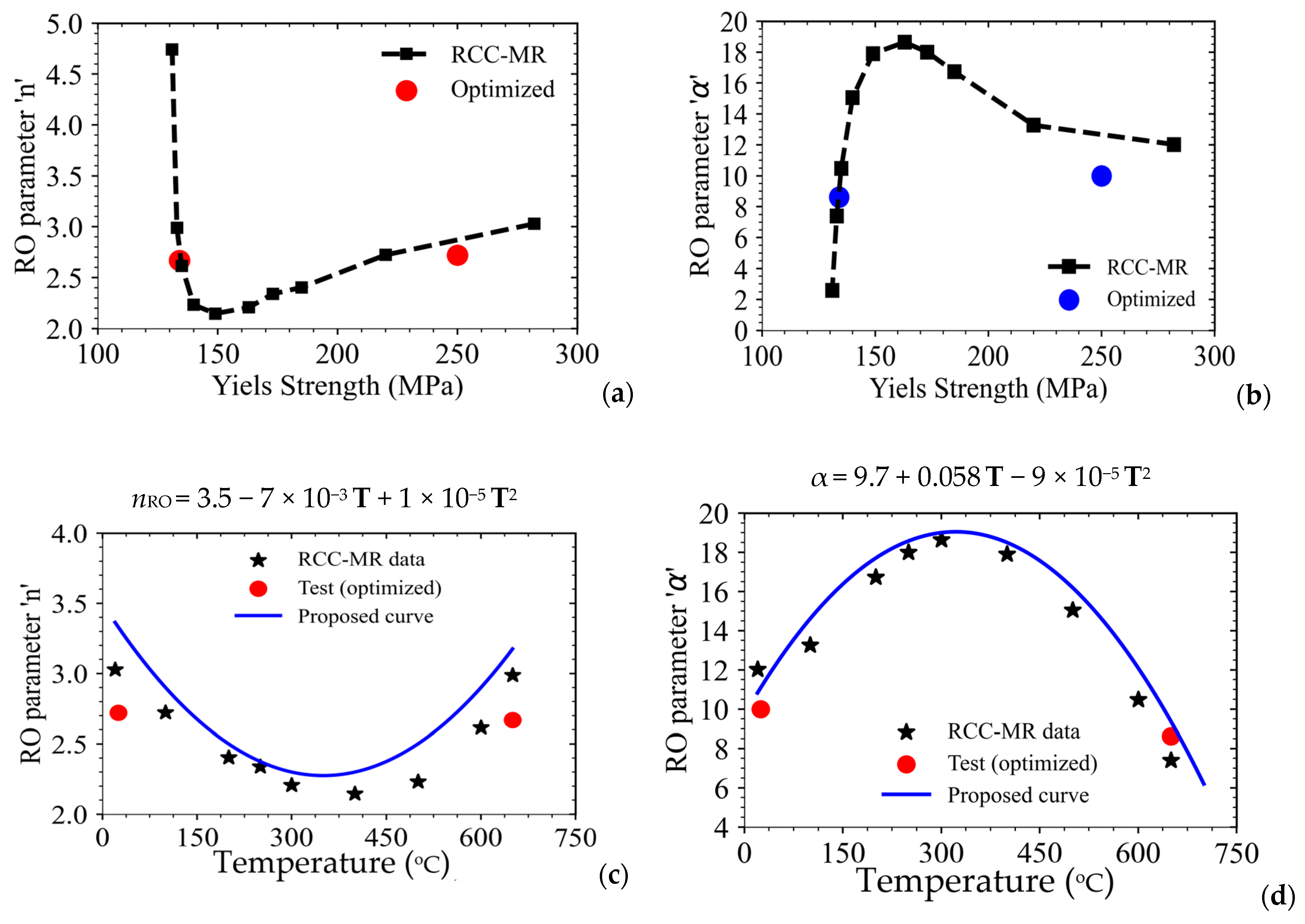
Hence, for completeness, the parameters ‘n’ and ‘α’ have been evaluated for the entire temperature range of 25–650 °C, and the corresponding data are presented in Figure 12. The variations of ‘n’ and ‘α’ with yield strength of the material (which change due to the test temperature) are presented in Figure 12a,b. The variations of ‘n’ and ‘α’ with test temperature have been plotted in Figure 12c,d and the corresponding expressions have been obtained, which can be used in FE simulations to obtain the material stress-strain curve at any intermediate value of temperature (for which the test data may not be available).

It may be noted that the values of Ramberg–Osgood parameters ‘$n_{\mathrm{RO}}$’ and ‘α’ as obtained from the new procedure adopted in this work match closely with those derived from RCC-MR data. The design curves provided in the RCC-MR code are not valid if the plastic strain in the component increases beyond the prescribed 1.5% limit. However, higher magnitudes of plastic strain, beyond this limit, are routinely encountered while analyzing regions with large geometrical discontinuities, such as shell-nozzle junctions, vessel heads, T-junctions, etc.

Generally, the design is carried out using the lower bound value of the stress-strain curve, and the life assessment is carried out using the average value of the stress-strain curve. Beyond the 1.5% limit of plastic strain, the stress-strain curves are provided at certain intervals of temperature only in the RCC-MR code. Conservatively, the next higher value of temperature is considered in the analysis if the design temperature of the component falls in between the intervals as provided in the code.

In addition, for thermo-mechanical analysis of structural components, temperature may vary significantly across the thickness of the components, and hence, a temperature-dependent material model for representing the true stress-strain curve of the material can be helpful for more accurate analysis in the form of a temperature-dependent Ramberg–Osgood parameter (n,α), instead of using the data at the next higher temperature (as provided in RCC-MR code), which can lead to significantly conservative results.

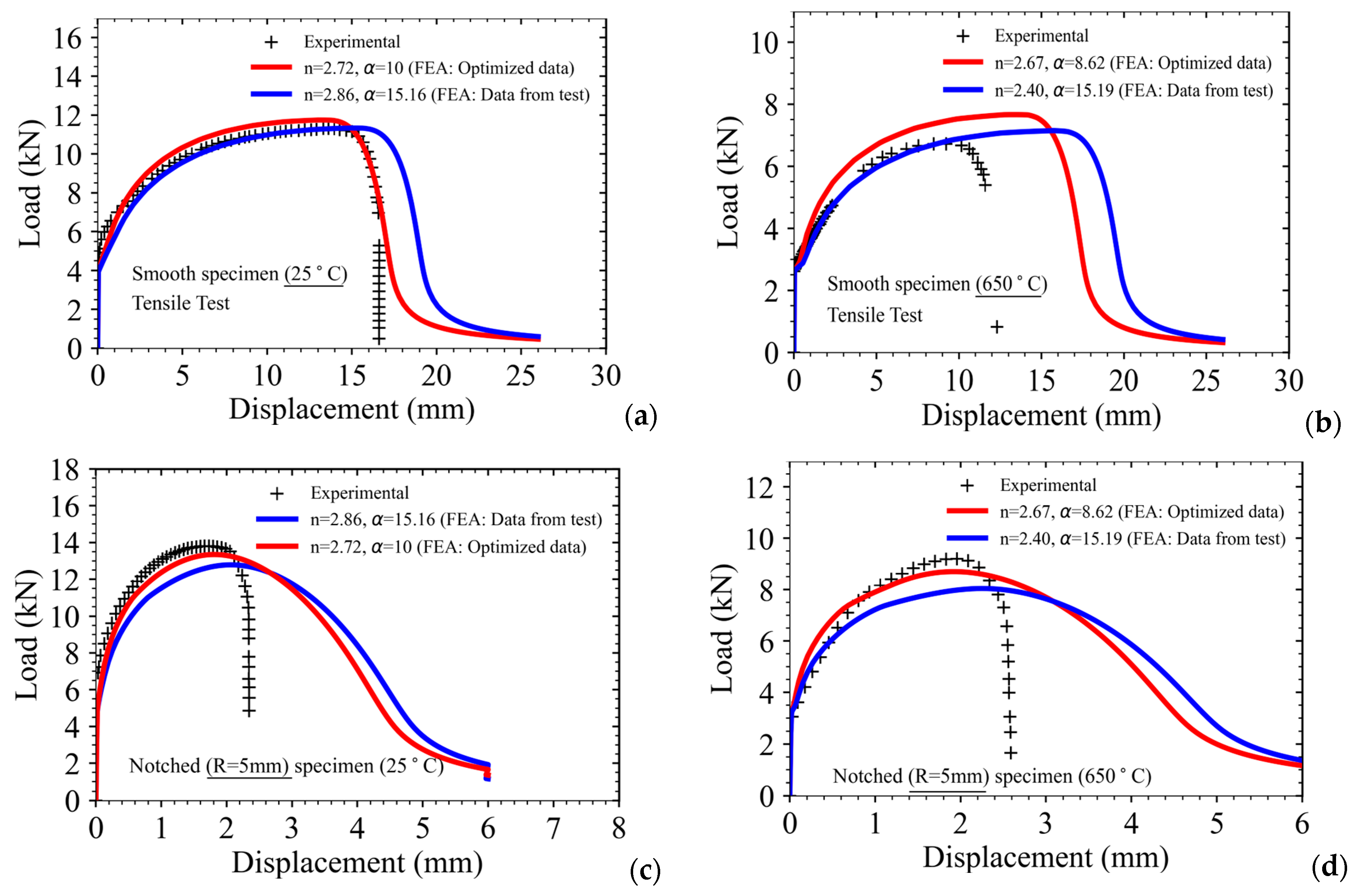
In order to validate the procedure and the parameters of the Ramberg–Osgood model, as derived from the new optimization procedure adopted in this work, the model has been used in an FE analysis of smooth as well as notched tensile specimens (with four different notch radii as reported earlier). The load-displacement results of all the specimens have been compared with those of the experiment at two different temperatures (i.e., 25 °C and 650 °C). For FE analysis, two different sets of Ramberg–Osgood parameters have been used, i.e., one set of parameters has been estimated using experimentally obtained stress-strain data of smooth tensile specimens (this is as per the conventional procedure discussed in the literature), and the second set is using the new optimization procedure as discussed earlier in this work.

The results of all types of specimens for the two test temperatures are presented in Figure 13a–h. It may be observed that the Ramberg–Osgood parameters, as evaluated following the new procedure, are able to model the load-displacement curves of all types of specimens at the two different temperatures very accurately, whereas the parameters, as evaluated following the conventional procedure, are inadequate in predicting the load-displacement behavior, especially of the notched specimens at both temperatures.

This discrepancy can be explained by considering the large scatter in data of smooth tensile specimens of SS316LN. One test or some limited test data may not be sufficient to model the material’s plastic hardening behavior, especially the plastic deformation in the presence of structural discontinuity such as notches and cracks, etc. The effect of stress triaxiality can be taken into account more accurately when considering smooth as well as notched specimen test data.

This is the reason why such a hybrid optimization procedure has been adopted in this work in order to evaluate the Ramberg–Osgood model accurately. This method can be easily extended for other engineering materials. In addition, it may be noted that the point of load drop (i.e., fracture strain for smooth specimens and fracture displacement for notched specimens) is not predicted accurately in this simulation (Figure 13a–h) as the damage initiation and propagation model is not included in the simulation. The fracture strain and the point of load drop in the tests in smooth as well as notched specimens at different temperatures can be predicted accurately through use of the Johnson–Cook damage model as presented in Equation (4). The corresponding results and discussions regarding this aspect have been presented in subsequent sections of this manuscript.

6. A New Procedure for Evaluation of Damage Parameters of the Johnson–Cook Model

In this section, the method of evaluation of damage parameters (i.e., d₁ to d₅ as presented through Equation (4)) of the Johnson–Cook material model has been presented. For evaluation of parameters d₁ to d₃, the data of smooth and notched tensile tests have been used along with the results of FE analysis. As stated earlier, it is easy to define the stress triaxiality and fracture strain from the test data of smooth tensile specimens due to the prevalence of a constant state of purely uniaxial stress throughout the cross-section (i.e., in the gauge region of the specimen).

However, for the notched specimens, the magnitude of stress triaxiality as well as plastic strain varies across the cross-section of the specimen. Hence, it is difficult to estimate the parameters of the Johnson–Cook damage model, as use of Equation (4) requires evaluation of a constant value of stress triaxiality and fracture strain from a given experiment. In order to address this issue, results of FE analysis have been used to simulate smooth and notched tensile specimens of different notch radii.

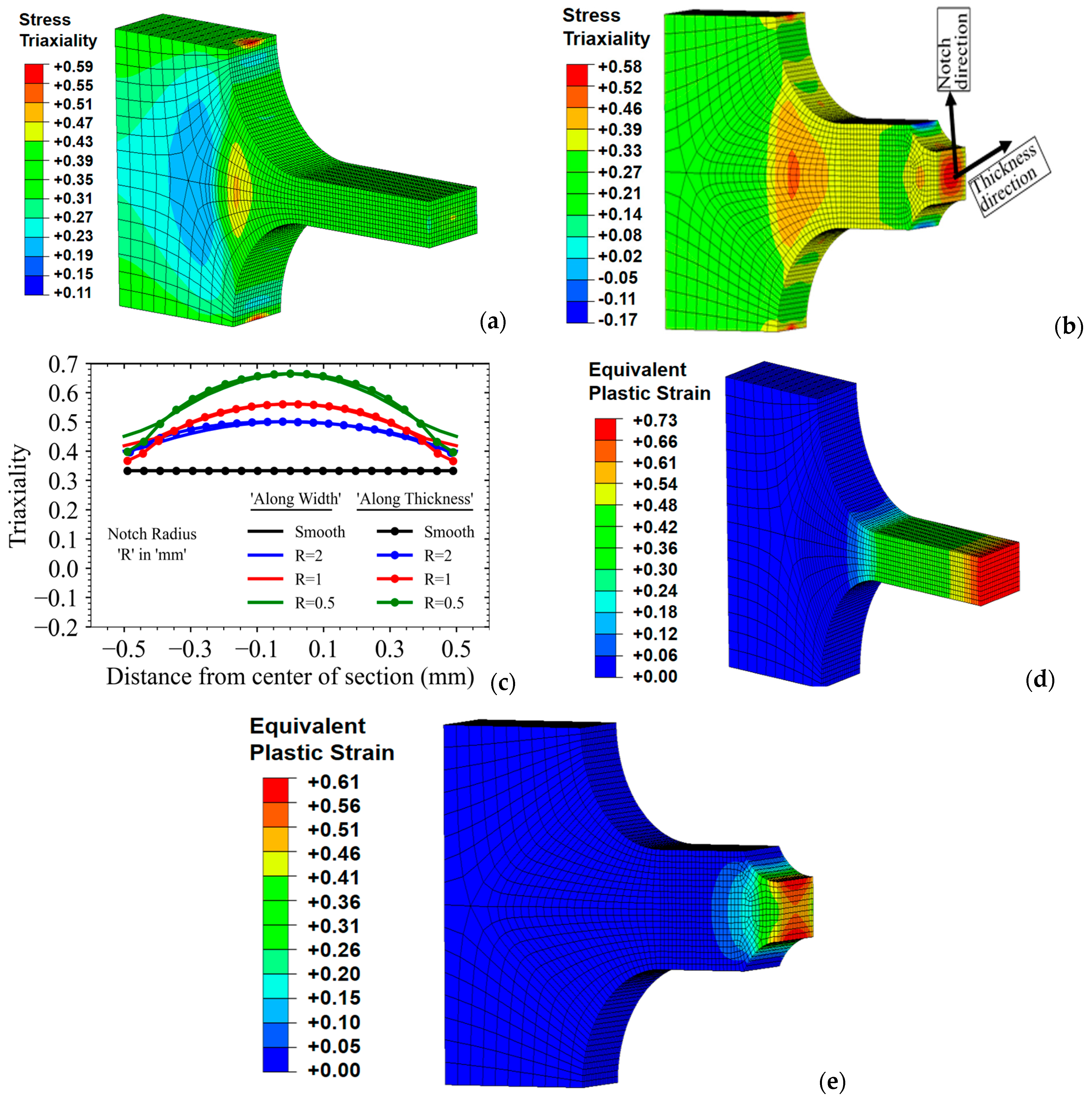
The contour of stress triaxiality in smooth and notched specimens (notch radius of 1 mm) for a given applied loading is shown in Figure 14a,b. It may be noted that the stress triaxiality for the smooth specimen is 1/3 (Figure 14a), whereas the stress triaxiality for the notched specimen (with a notch radius of 1 mm) is much higher. Its maximum value is approximately 0.58, which occurs at the central region of the minimum cross-sectional area of the notched specimen as shown in Figure 14b.

The spatial variations of stress triaxiality, along both the thickness and notch or width directions of the specimens, for various values of notch radii, are shown in Figure 14c. It may be noted that the stress triaxiality is maximum at the center for each notched specimen, and it decreases along both directions from the center to the surface. In addition, the stress triaxiality magnitude at the center of the notched specimen is highest for the specimen with the lowest notch radius and vice versa.

This can be explained by the phenomenon that decreasing the notch radius (while keeping all the other dimensions the same) increases the localized constraint, and this in turn restricts the plastic deformation in the notched region of the specimen. The equivalent plastic strain contour has been plotted for both the smooth and notched specimens in Figure 14d,e for a given applied loading.

It can be observed that the magnitude of equivalent plastic strain is lesser at the center of the notched region when compared to those at the free surfaces, whereas, for smooth specimens, it is constant, representing a pure uniaxial state of plastic deformation. The spatial variation of equivalent plastic strain magnitudes can again be explained on the basis of the spatial variation of stress triaxiality (more is the equivalent plastic strain for a lesser value of stress triaxiality and vice versa).

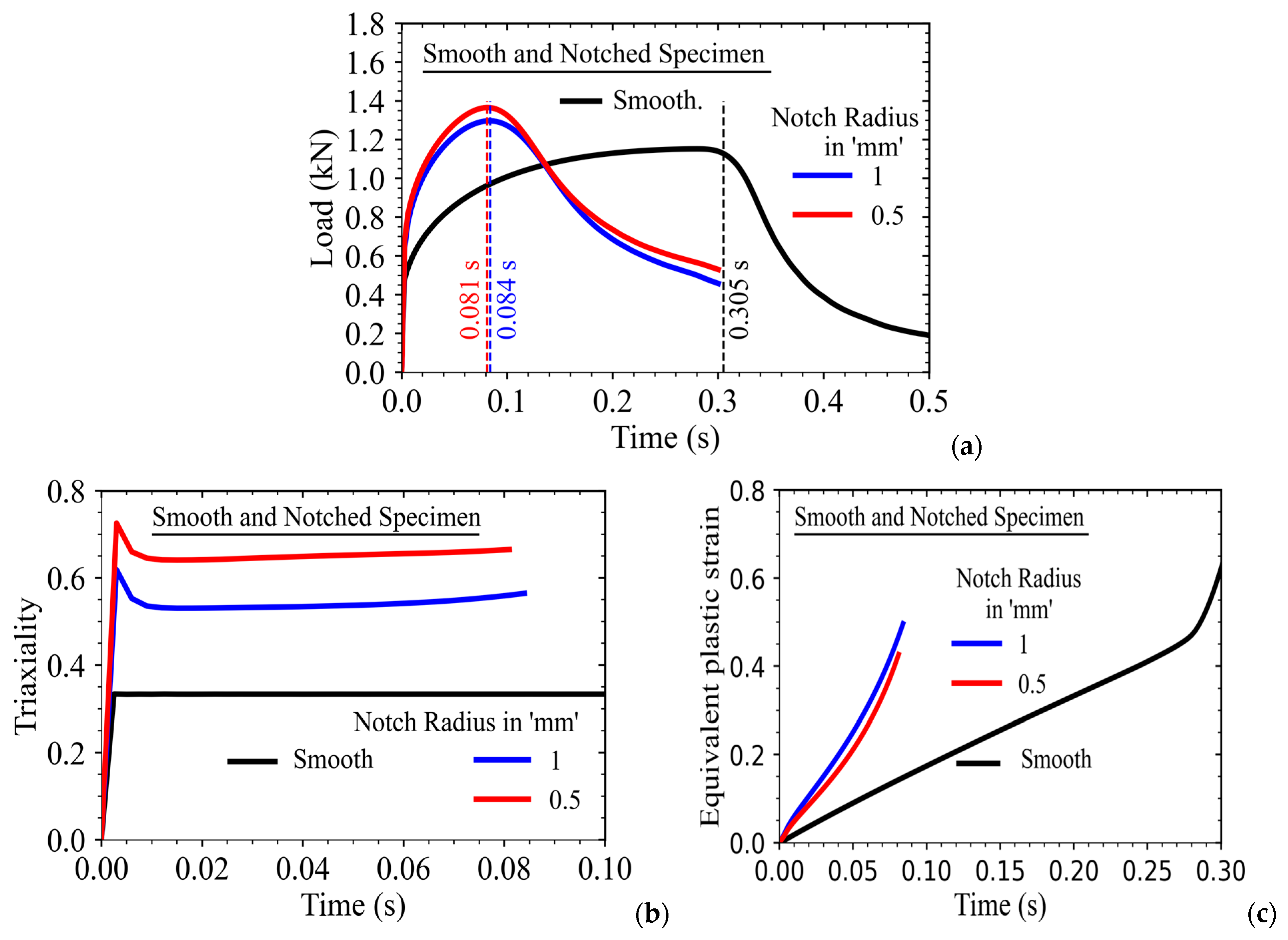
The data of the maximum value of stress triaxiality at the central notched region of the smooth as well as the notched specimens (with different notch radii) as obtained from FE analysis have been used further in Equation (4) to evaluate the parameters d₁ to d₃ of the Johnson–Cook damage model. The displacements at which these parameters have been evaluated are shown in typical load-time graphs of the tensile specimens as presented in Figure 15a.

It may be noted that a drastic load drop occurs (after necking in the specimen) in SS316LN tensile tests conducted at room temperature, and hence, these instances of initiation of necking in these specimens have been used to evaluate the characteristic values of stress triaxiality and equivalent plastic strain (corresponding to fracture initiation). The stress triaxiality values almost remain constant during plastic deformation for all the types of specimens, as shown in Figure 15b; however, the magnitude of stress triaxiality increases with a decrease in the magnitude of the notch radius, and these are much higher compared to that of the smooth specimen.

The equivalent plastic strain magnitude (at the center of the notched region for the notched specimens) also increases with applied displacement loading for all types of specimens, as presented in Figure 15c; however, the magnitudes for equivalent plastic strain are lower for the notched specimen with a lesser notch radius (for a given applied displacement loading), as this represents higher stress triaxiality, more constraint, and hence, lesser plastic deformation.

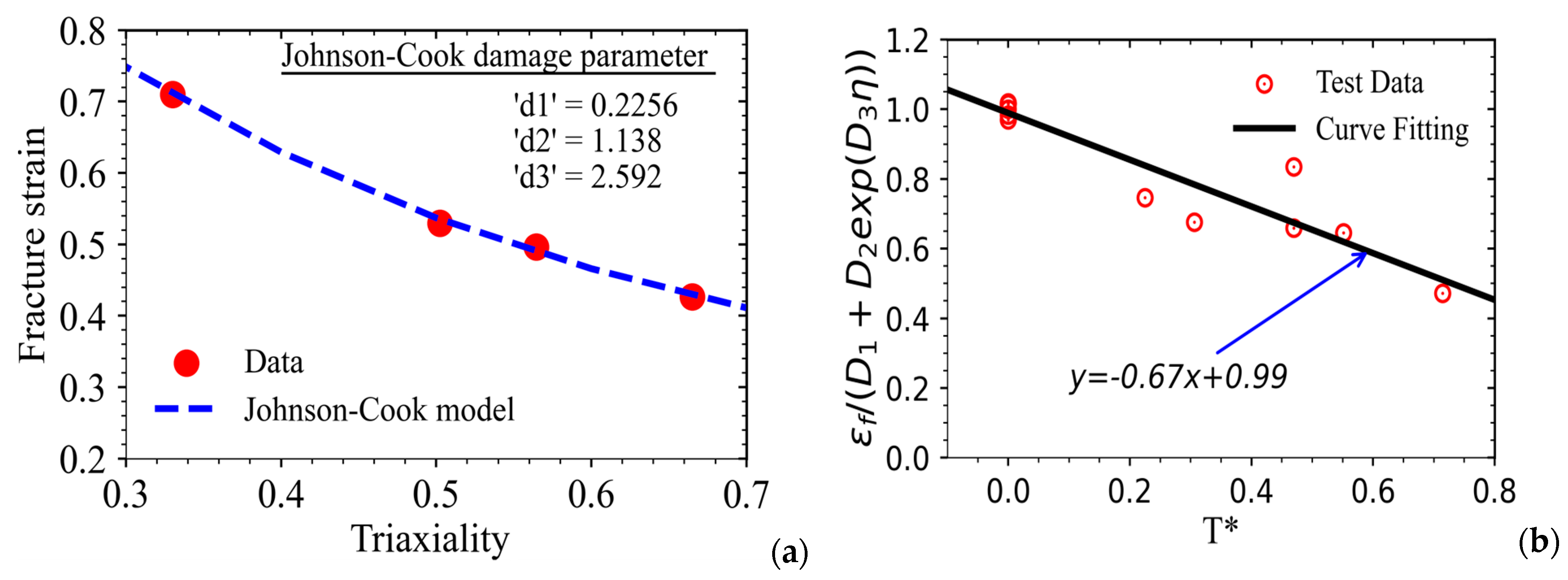
These data of stress triaxiality and equivalent plastic strain for smooth and notched specimens have been used in the first term of Equation (4) to evaluate the damage parameters d₁ to d₃. As these tests are conducted at room temperature (also taken as reference temperature in the model) and quasi-static loading conditions (i.e., the strain rate is the same as the reference strain rate in the model), the second and third terms of Equation (4) become unity.

This makes it easier to estimate the parameters d₁ to d₃ of the model using the first term of Equation (4) as shown in Figure 16a. Once the parameters d₁ to d₃ are estimated from the results of FE analysis and quasi-static room temperature test data, the temperature-dependent damage parameter d₅ has been evaluated using the high-temperature test data (i.e., fracture strain) of smooth tensile specimens as presented in Figure 1d for temperatures ranging from 25 °C to 1000 °C.

The third term of Equation (4) has been used for this purpose as the second term becomes unity because of the quasi-static nature of the tests. The result of the estimation of the parameter d₅ from the test data are presented in Figure 16b, where the parameter d₅ has been estimated to be −0.67, representing the slope of the curve in a log-log scale. The accuracy of this temperature-dependent damage parameter has been assessed in the next section by comparing the results of the FE simulation of tensile specimens at different temperatures with those of test data.

7. Discussion

As we have discussed earlier, while following the procedure for evaluation of the parameter ‘m’, the conventional procedure does not provide an accurate estimate of the temperature-dependent damage parameter d₅. Hence, we have adopted here the principle of minimization of error (where the error is measured in terms of the absolute difference of the area between the load-displacement data as obtained from FE simulation and from those of the experiment) in order to evaluate the above parameter. The results of the FE simulation and experiment have been used in order to evaluate the error. The value of error as a function of damage parameter d₅ has been presented in

Table 4. Variation of absolute difference in area of load-displacement curves of experiment and FE analysis for various values of parameter d₅.

Value of Parameter d5	Area_Experiment (kN-mm)	Area_FEA (kN-mm)	Error = Absolute Difference (kN-mm)
−0.6	11.14	12.71	1.58
−1.1	11.14	12.48	1.35
−1.6	11.14	11.82	0.69
−2.1	11.14	10.07	1.06
−2.6	11.14	8.23	2.91

, where the damage parameter has been varied in the range of −0.6 to −2.6.

This range also covers the conventionally estimated magnitude of d₅ (i.e., −0.67). It may be noted that the error initially reduces with the increase in the negative value of parameter d₅, and then it increases again. The more negative value of d₅ reduces the area under the load-displacement curve of the tensile specimen as obtained from FE analysis. The use of a higher d₅ value in the FE analysis also results in earlier necking (and a corresponding drastic load drop) in the specimen, and hence, this results in a lower fracture strain in the simulation. For a particular value of the parameter d₅, the error becomes minimum, and this corresponds to the most suitable parameter d₅ for the material.

The load-displacement results, as obtained from the FE simulation of smooth tensile specimens at a temperature of 300 °C, are presented in Figure 17a for various magnitudes of parameter d₅ (while keeping all the other damage parameters unchanged). It can be observed that the displacement at fracture (which corresponds to the point of drastic load drop in the simulation) decreases with an increase in the (negative) value of the parameter d₅, indicating a lower value of fracture strain for a higher value of d₅.

The results from the FE simulation have also been compared with experimental data for 300 °C and the absolute error in the area of load-displacement data (between FE simulation and experiment) has been plotted as a function of parameter d₅ in Figure 17b. The error initially reduces with an increase in the negative value of d₅, and then it increases again. At a value of d₅ = −1.7, the error is minimal, and this value has been used as the actual temperature-dependent material damage parameter of the Johnson–Cook model for SS316LN.

The accuracy and the validity of the parameter d₅ have been demonstrated by comparing the load-displacement data of smooth as well as notched tensile specimens tested at different temperatures. Not only the material hardening curve but also the fracture points at different temperatures as predicted by FE simulations have been compared with the corresponding experimental data, and these are presented in Figure 17c–h.

Two different values of the damage parameter d₅ have been used in the FE simulations. One value of d₅ is −0.67, which is the same as estimated using the conventional technique (as discussed in the literature), and the other value of d₅ is −1.7, which has been evaluated using the new error minimization technique, which involves combined FE analysis and experimental data at different test temperatures.

It can be observed from Figure 17c–h that the value of d₅, as evaluated using the new error minimization technique, provides a very accurate prediction of fracture strains of all types of specimens (i.e., smooth and notched) at different temperatures, whereas the value of parameter d₅ as evaluated using the conventional technique is inadequate in modeling the material’s plastic deformation behavior and the evolution of ductile damage (which correlates with fracture strain) in the material at different temperatures. Hence, it is recommended that the new procedure, as demonstrated in this work, be used for accurate evaluation of both the plasticity and damage parameters of different types of material constitutive models. The different parameters of the Johnson–Cook plasticity and damage model, as evaluated for the austenitic grade stainless steel SS316LN (material of construction of core components of the Indian PFBR), are presented in

Table 5. Johnson–Cook plasticity and damage parameters for austenitic strainless steel SS316LN used in Indian PFBR.

Johnson–Cook Plasticity Parameters
Parameter	Value
A	200 MPa
B	1160 MPa
n	0.59
C (ref. strain rate = 1 × 10−3/s)	0.03
m (Tref = 25 °C)	1.18
Johnson–Cook damage Parameters
d1	0.225
d2	1.138
d3	2.592
d5 (Tref = 25 °C)	−1.7

.

8. Summary and Conclusions

In this work, a new optimization procedure has been presented for evaluation of the parameters of Johnson–Cook plasticity and damage models, respectively. Extensive tests, using smooth and notched tensile specimens at different temperatures as well as different strain rates (high strain rate tests have been carried out using a split Hopkinson pressure bar test setup), have been conducted in order to evaluate the material parameters. The new procedure developed in this work is able to evaluate the Johnson–Cook model parameters accurately, and hence, these parameters, when used in the FE simulation, are able to model both the material plastic deformation as well as the fracture strain accurately over a wide range of temperature, strain rates, and stress triaxialities. The following conclusions can be derived from this work.

• The conventional procedure for parameter estimation provides inaccurate results, which is due to the presence of large scatter in data (especially for parameter ‘m’) and inaccurate estimation of damage initiation strain as a function of temperature (i.e., for the parameter d₅).
• The new procedure involving error minimization is accurate as it takes care of the deformation behavior of different types of specimens in the analysis, which represents a wide range of stress triaxialities.
• The values of temperature-dependent parameters ‘m’ and ‘d₅’, as estimated from the use of the new optimization technique, have been found to be 1.18 and −1.7, respectively, for SS316LN.
• For the high strain rate tests, as conducted using a split Hopkinson pressure bar test setup, FE analysis for identification of parameter ‘C’ (as followed in this work) is more appropriate as it takes care of the inherently varying strain rate nature of the test.
• The optimization method followed in this work is more general as it involves FE analysis of the actual deformation behavior of different types of specimens (i.e., smooth and notched tensile), and hence, it can be used for estimation of parameters of Johnson–Cook as well as Ramberg–Osgood models.

References

1. Kale, R.D. India’s fast breeder reactor programme—A review and critical assessment. Prog. Nucl. Energy 2020, 122, 103265. [Google Scholar] [CrossRef]
2. Bharasi, N.S.; Krishna, N.G.; Shankar, A.R.; Krishnakumar, S.; Chandramouli, S.; Karki, V.; Kannan, S.; Philip, J. Influence of long term Sodium Exposure on the Corrosion and Tensile Properties of AISI Type 316LN stainless steel and modified 9Cr-1Mo steel. J. Nucl. Mater. 2022, 567, 153830. [Google Scholar]
3. RCC-MR 2020: Design and Construction Rules for Mechanical Components of Nuclear Installations; AFCEN: Paris, France; CEA: Paris, France, June 2020.
4. Johnson, G.R.; Cook, W.H. A constitutive model and data for metals subjected to large strains, high strain rates and high temperatures. In Proceedings of the Seventh International Symposium on Ballistics, The Hague, The Netherlands, 19–21 April 1983; pp. 541–547. [Google Scholar]
5. Sgobba, S.; Libeyre, P.; Marcinek, D.J.; Nyilas, A. A Comparative Assessment of Metallurgical and Mechanical Properties of Two Austenitic Stainless Steels for the Conductor Jacket of the ITER Central Solenoid. Fusion Eng. Des. 2013, 88, 2484–2487. [Google Scholar] [CrossRef]
6. Qin, J.; Dai, C.; Liao, G.; Wu, Y.; Zhu, X.; Huang, C.; Li, L.; Wang, K.; Shen, X.; Tu, Z.; et al. Tensile test of SS 316LN jacket with different conditions. Cryogenics 2014, 64, 16–20. [Google Scholar] [CrossRef]
7. Fedoriková, A.; Petroušek, P.; Kvačkaj, T.; Kočiško, R.; Zemko, M. Development of Mechanical Properties of Stainless Steel 316LN-IG after Cryo-Plastic Deformation. Materials 2023, 16, 6473. [Google Scholar] [CrossRef]
8. Petrousek, P.; Kvackaj, T.; Kocisko, R.; Bidulska, J.; Luptak, M.; Manfredi, D.; Grande, M.A.; Bidulsky, R. Influence of Cryorolling on Properties of L-Pbf 316l Stainless Steel Tested at 298k and 77k. Acta Metall. Slovaca 2019, 25, 283–290. [Google Scholar] [CrossRef]
9. Han, W.; Liu, Y.; Wan, F.; Liu, P.; Yi, X.; Zhan, Q.; Morrall, D.; Ohnuki, S. Deformation Behavior of Austenitic Stainless Steel at Deep Cryogenic Temperatures. J. Nucl. Mater. 2018, 504, 29–32. [Google Scholar] [CrossRef]
10. Zhang, H.; Huang, C.; Huang, R.; Li, L. Influence of pre-strain on cryogenic tensile properties of 316LN austenitic stainless steel. Cryogenics 2020, 106, 103058. [Google Scholar] [CrossRef]
11. Wu, S.; Xin, J.; Xie, W.; Zhang, H.; Huang, C.; Wang, W.; Zhou, Z.; Zhou, Y.; Li, L. Mechanical properties and microstructure evolution of cryogenic pre-strained 316LN stainless steel. Cryogenics 2022, 121, 103388. [Google Scholar] [CrossRef]
12. Wei, Y.; Lu, Q.; Kou, Z.; Feng, T.; Lai, Q. Microstructure and strain hardening behavior of the transformable 316L stainless steel processed by cryogenic pre-deformation. Mater. Sci. Eng. A 2023, 862, 144424. [Google Scholar] [CrossRef]
13. Kim, M.-S.; Lee, T.; Park, J.-W.; Kim, Y. Tensile and Fracture Characteristics of 304L Stainless Steel at Cryogenic Temperatures for Liquid Hydrogen Service. Metals 2023, 13, 1774. [Google Scholar] [CrossRef]
14. Weiss, K.-P.; Kraskowski, A.; Koukolíková, M.; Podaný, P.; Zemko, M. Mechanical properties after thermomechanical processing of cryogenic high-strength materials for magnet application. Fusion Eng. Des. 2021, 168, 112599. [Google Scholar] [CrossRef]
15. Kvackaj, T.; Rozsypalova, A.; Kocisko, R.; Bidulska, J.; Petrousek, P.; Vlado, M.; Pokorny, I.; Sas, J.; Weiss, K.-P.; Duchek, M. Influence of Processing Conditions on Properties of AISI 316LN Steel Grade. J. Mater. Eng. Perform. 2020, 29, 1509–1514. [Google Scholar] [CrossRef]
16. Lorenzetto, P.; Helie, M.; Molander, A. Stress Corrosion Cracking of AISI 316LN Stainless Steel in ITER Primary Water Conditions. J. Nucl. Mater. 1996, 233, 1387–1392. [Google Scholar] [CrossRef]
17. Yang, W.; Cheng, P.; Li, Y.; Wang, R.; Liu, G.; Xin, L.; Zhang, J.; Sun, J. Ratcheting-Induced Twinning/de-Twinning Behaviors in a 316LN Austenitic Stainless Steel. Mater. Sci. Eng. A 2022, 851, 143648. [Google Scholar] [CrossRef]
18. Üçok, İ.; Ando, T.; Grant, N.J. Property Enhancement in Type 316L Stainless Steel by Spray Forming. Mater. Sci. Eng. A 1991, 133, 284–287. [Google Scholar] [CrossRef]
19. Wegener, T.; Wu, T.; Sun, F.; Wang, C.; Lu, J.; Niendorf, T. Influence of Surface Mechanical Attrition Treatment (SMAT) on Microstructure, Tensile and Low-Cycle Fatigue Behavior of Additively Manufactured Stainless Steel 316L. Metals 2022, 12, 1425. [Google Scholar] [CrossRef]
20. Petrousek, P.; Kvackaj, T.; Bidulska, J.; Bidulsky, R.; Grande, M.A.; Manfredi, D.; Weiss, K.-P.; Kocisko, R.; Luptak, M.; Pokorny, I. Investigation of the Properties of 316L Stainless Steel after AM and Heat Treatment. Materials 2023, 16, 3935. [Google Scholar] [CrossRef] [PubMed]
21. Herrera, C.; Plaut, R.L.; Padilha, A.F. Microstructural Refinement during Annealing of Plastically Deformed Austenitic Stainless Steels. Mater. Sci. Forum 2007, 550, 423–428. [Google Scholar] [CrossRef]
22. Hwang, I.-S.; So, T.-Y.; Lee, D.-H.; Shin, C.-S. Characterization of Mechanical Properties and Grain Size of Stainless Steel 316L via Metal Powder Injection Molding. Materials 2023, 16, 2144. [Google Scholar] [CrossRef]
23. Uralde, V.; Suarez, A.; Aldalur, E.; Veiga, F.; Ballesteros, T. Wall Fabrication by Direct Energy Deposition (DED) Combining Mild Steel (ER70) and Stainless Steel (SS 316L): Microstructure and Mechanical Properties. Materials 2022, 15, 5828. [Google Scholar] [CrossRef]
24. Shang, Z.; Fan, C.; Ding, J.; Xue, S.; Gabriel, A.; Shao, L.; Voisin, T.; Wang, Y.M.; Niu, T.; Li, J.; et al. Heavy ion irradiation response of an additively manufactured 316LN stainless steel. J. Nucl. Mater. 2021, 546, 152745. [Google Scholar] [CrossRef]
25. Sumanariu, C.A.; Amza, C.G.; Baciu, F.; Vasile, M.I.; Nicoara, A.I. Comparative Analysis of Mechanical Properties: Conventional vs. Additive Manufacturing for Stainless Steel 316L. Materials 2024, 17, 4808. [Google Scholar] [CrossRef] [PubMed]
26. Lesley, R.; Herrera, C.; Escriba, D.; Rios, P.; Padilha, A. A Short Review on Wrought Austenitic Stainless Steels at High Temperatures: Processing, Microstructure, Properties and Performance. Mater. Res. 2007, 10, 453–460. [Google Scholar]
27. Weiss, B.; Stickler, R. Phase Instabilities during High Temperature Exposure of 316 Austenitic Stainless Steel. Met. Trans. 1972, 3, 851–866. [Google Scholar] [CrossRef]
28. Singhal, L.K.; Martin, J.W. The Formation of Ferrite and Sigma-Phase in Some Austenitic Stainless Steels. Acta Metall. 1968, 16, 1441–1451. [Google Scholar] [CrossRef]
29. Wasnik, D.N.; Dey, G.K.; Kain, V.; Samajdar, I. Precipitation Stages in a 316L Austenitic Stainless Steel. Scr. Mater. 2003, 49, 135–141. [Google Scholar] [CrossRef]
30. Tabin, J. Kinematic and Thermal Characteristic of Discontinuous Plastic Flow in Metastable Austenitic Stainless Steels. Mech. Mater. 2021, 163, 104090. [Google Scholar] [CrossRef]
31. Lu, Q.; Zhang, C.; Wang, W.; Jiang, S.; Aucott, L.; Yasmeen, T.; Jiang, J. Reveal the Viscoplastic Behaviour and Microstructure Evolution of Stainless Steel 316L. Materials 2022, 15, 7064. [Google Scholar] [CrossRef] [PubMed]
32. Lu, W.; Hua, X.; Zhou, X.; Huang, J.; Peng, X. Aging precipitation behaviors of Nb-contained 316LN SS. J. Alloys Compd. 2017, 701, 993–1002. [Google Scholar] [CrossRef]
33. Spruiell, J.E.; Scott, J.A.; Ary, C.S.; Hardin, R.L. Microstructural Stability of Thermal-Mechanically Pretreated Type 316 Austenitic Stainless Steel. Met. Trans. 1973, 4, 1533–1544. [Google Scholar] [CrossRef]
34. Prasad Reddy, G.V.; Christopher, J.; Praveen, C.; Ganesan, V. Creep deformation and constitutive modelling of 316LN SS with varying nitrogen content. Mater. Today Proc. 2024, 108, 86–92. [Google Scholar] [CrossRef]
35. Ganesan, V.; Ganesh Kumar, J.; Laha, K.; Mathew, M.D. Notch creep rupture strength of 316LN SS and its variation with nitrogen content. Nucl. Eng. Des. 2013, 254, 179–184. [Google Scholar] [CrossRef]
36. Ganesh Kumar, J.; Ganesan, V.; Laha, K.; Mathew, M.D. Time dependent design curves for a high nitrogen grade of 316LN stainless steel for fast reactor applications. Nucl. Eng. Des. 2013, 265, 949–956. [Google Scholar] [CrossRef]
37. Ding, J.; Tan, J.; Zhang, Z.; Wang, X.; Wu, X.; Han, E.-H.; Ke, W. Low cycle fatigue behavior of 316LN stainless steel hollow specimen in air and liquid lead–bismuth eutectic. Int. J. Fatigue 2023, 175, 107812. [Google Scholar] [CrossRef]
38. Yang, J.; Li, B.; Zheng, Y.; Chen, G.; Chen, X. Low cycle fatigue behavior of additive manufactured 316LN stainless steel at 550 °C: Effect of solution heat treatment. Int. J. Fatigue 2024, 179, 108066. [Google Scholar] [CrossRef]
39. Li, B.; Zheng, Y.; Zhao, J.; Shi, S.; Zhang, Z.; Chen, X. Cyclic deformation behavior and dynamic strain aging of 316LN stainless steel under low cycle fatigue loadings at 550 °C. Mater. Sci. Eng. A 2021, 818, 141411. [Google Scholar] [CrossRef]
40. Lin, Q.; Chen, X.; Zheng, Y.; Zhang, Z.; Chen, G.; Li, B. Multiaxial isothermal and thermomechanical fatigue behavior of 316LN stainless steel. Int. J. Press. Vessel. Pip. 2022, 197, 104633. [Google Scholar] [CrossRef]
41. Zheng, Y.; Chen, X.; Zhang, Z.; Shi, S.; Chen, G.; Li, B. Multiaxial low cycle fatigue behavior and life prediction method of 316LN stainless steel at 550 °C. Int. J. Fatigue 2022, 156, 106637. [Google Scholar] [CrossRef]
42. Li, B.; Zheng, Y.; Chen, G.; Itoh, T.; Chen, X. Isothermal and thermomechanical fatigue behavior of 316LN stainless Steel: Effects of strain amplitude. Int. J. Fatigue 2023, 166, 107304. [Google Scholar] [CrossRef]
43. Zheng, Y.; Li, B.; Wang, F.; Xu, C.; Wang, K.; Chen, X. Isothermal and thermo-mechanical fatigue crack growth behavior and modelling of 316LN stainless steel with the superposition of HCF loading. Int. J. Fatigue 2024, 189, 108548. [Google Scholar] [CrossRef]
44. Ma, Y.; Zhang, Z.; Tan, J.; Wu, X.; Wang, X.; Wang, Y.; Han, E.-H.; Ke, W. Microstructurally and mechanically small fatigue crack growth behaviors of 316LN stainless steel in high-temperature pressurized water. Corros. Sci. 2024, 227, 111735. [Google Scholar] [CrossRef]
45. Ma, Y.; Zhang, Z.; Zhang, X.; Yin, H.; Liang, B.; Tan, J.; Wu, X.; Han, E.-H.; Ke, W. Effects of strain rate on low-cycle fatigue crack growth behavior of 316LN weld metal in high-temperature pressurized water. Corros. Sci. 2022, 199, 110169. [Google Scholar] [CrossRef]
46. Praveen, C.; Christopher, J.; Ganesan, V.; Prasad Reddy, G.V.; Sasikala, G.; Albert, S.K. Constitutive modelling of transient and steady state creep behaviour of type 316LN austenitic stainless steel. Mech. Mater. 2019, 137, 103122. [Google Scholar] [CrossRef]
47. Xing, R.; Sun, X.; Chen, X. Cyclic constitutive modeling of 316LN stainless steel considering thermal aging mechanism. Eur. J. Mech.—A/Solids 2024, 107, 105392. [Google Scholar] [CrossRef]
48. Praveen, C.; Christopher, J.; Ganesan, V.; Prasad Reddy, G.V.; Choudhary, B.K. Dislocation density based modeling of three-stage work hardening behaviour of type 316LN SS with varying nitrogen content and its finite element implementation for different notch radii. Mater. Chem. Phys. 2020, 241, 122342. [Google Scholar] [CrossRef]
49. Li, X.Q.; Zhao, J.J.; Xu, J.C.; Liu, X. Mechanical Properties and Defective Effects of 316LN Stainless Steel by First-Principles Simulations. J. Mater. Sci. Technol. 2011, 27, 1029–1033. [Google Scholar] [CrossRef]
50. Sidharth, R.; Nikhil, R.; Krishnan, S.A.; Keralavarma, S.M.; Moitra, A.; Vasudevan, M. Crack initiation and growth in 316LN stainless steel: Experiments and XFEM simulations. Eng. Fract. Mech. 2022, 274, 108770. [Google Scholar] [CrossRef]
51. Xiong, L.; You, Z.S.; Lu, L. Fracture behavior of an austenitic stainless steel with nanoscale deformation twins. Scr. Mater. 2017, 127, 173–177. [Google Scholar] [CrossRef]
52. Sakurai, T.; Umezawa, O. Fracture toughness and martensitic transformation in type 316LN austenitic stainless steel extra-thick plates at 4.2 K. Mater. Sci. Eng. A 2023, 862, 144122. [Google Scholar] [CrossRef]
53. Xin, J.; Fang, C.; Huang, C.; Yang, W.; Dai, W.; Zhang, H.; Wei, J.; Li, L.; Wu, J.; Song, Y. Analysis of the fracture mechanism at cryogenic temperatures of thick 316LN laser welded joints. Fusion Eng. Des. 2019, 148, 111277. [Google Scholar] [CrossRef]
54. Ganesh Kumar, J.; Prasad Reddy, G.V.; George, A.; Saikumaran, A.; Mythili, R.; Anil Kumar, P.; Das Gupta, A.; Vasudevan, M. Evaluation of tensile properties of thermally aged 316LN stainless steel with varying nitrogen content using ABI technique. Mater. Sci. Eng. A 2021, 806, 140819. [Google Scholar] [CrossRef]
55. Ragavendran, M.; Ganesh Kumar, J.; Vasudevan, M. Evaluation of tensile properties using uniaxial and ball indentation testing and correlation with microstructure variations across the 316LN stainless steel weld joints. Mater. Sci. Eng. A 2022, 832, 142445. [Google Scholar] [CrossRef]
56. Astafurova, E.; Fortuna, A.; Melnikov, E.; Astafurov, S. The Effect of Strain Rate on Hydrogen-Assisted Deformation Behavior and Microstructure in AISI 316L Austenitic Stainless Steel. Materials 2023, 16, 2983. [Google Scholar] [CrossRef] [PubMed]
57. Khaleghifar, F.; Razeghi, K.; Heidarzadeh, A.; Taherzadeh Mousavian, R. Effect of Hydrogen on the Tensile Behavior of Austenitic Stainless Steels 316L Produced by Laser-Powder Bed Fusion. Metals 2021, 11, 586. [Google Scholar] [CrossRef]
58. Gurson, A.L. Continuum theory of ductile rupture by void nucleation and growth: Part I—Yield criteria and flow rules for porous ductile media. J. Eng. Mater. Technol. 1977, 99, 2–19. [Google Scholar] [CrossRef]
59. Needleman, A.; Tvergaard, V. An analysis of ductile rupture in notched bars. J. Mech. Phys. Solids 1984, 32, 461–490. [Google Scholar] [CrossRef]
60. Lemaitre, J. A continuous damage mechanics model for ductile fracture. J. Eng. Mater. Technol. 1985, 107, 83–89. [Google Scholar] [CrossRef]
61. Takuda, H.; Mori, K.; Fujimoto, H.; Hatta, N. Prediction of forming limit in bore-expanding of sheet metals using ductile fracture criterion. J. Mater. Process. Technol. 1999, 92, 433–438. [Google Scholar] [CrossRef]
62. Bao, Y.; Wierzbicki, T. On fracture locus in the equivalent strain and stress triaxiality space. Int. J. Mech. Sci. 2004, 46, 81–98. [Google Scholar] [CrossRef]
63. Bao, Y.; Wierzbicki, T. On the cut-off value of negative triaxiality for fracture. Eng. Fract. Mech. 2005, 72, 1049–1069. [Google Scholar] [CrossRef]
64. Bai, Y.; Wierzbicki, T. A new model of metal plasticity and fracture with pressure and Lode dependence. Int. J. Plast. 2008, 24, 1071–1096. [Google Scholar] [CrossRef]
65. Bai, Y.; Wierzbicki, T. Application of extended Mohr-Coulomb criterion to ductile fracture. Int. J. Fract. 2010, 161, 1–20. [Google Scholar] [CrossRef]
66. Wu, B.; Li, X.; Di, Y.; Brinnel, V.; Lian, J.; Münstermann, S. Extension of the modified Bai-Wierzbicki model for predicting ductile fracture under complex loading conditions. Fatigue Fract. Eng. Mater. Struct. 2017, 40, 2152–2168. [Google Scholar] [CrossRef]
67. Sadeghi Nezhad, M.S.; Haji Aboutalebi, F. A 2D Lode improved Lemaitre’s ductile damage model for damage prediction in ductile sheet metals under various loading conditions. Eng. Fail. Anal. 2024, 164, 108609. [Google Scholar] [CrossRef]
68. Haji Aboutalebi, F.; Poursina, M.; Nejatbakhsh, H.; Khataei, M. Numerical simulations and experimental validations of a proposed ductile damage model for DIN1623 St12 steel. Eng. Fract. Mech. 2018, 192, 276–289. [Google Scholar] [CrossRef]
69. Gao, J.; He, T.; Huo, Y.; Song, M.; Yao, T.; Yang, W. Comparison of modified Mohr-Coulomb model and Bai-Wierzbicki model for constructing 3D ductile fracture envelope of AA6063. Chin. J. Mech. Eng. 2021, 34, 35. [Google Scholar] [CrossRef]
70. Behrens, B.; Rosenbusch, D.; Wester, H.; Althaus, P. Comparison of three different ductile damage models for deep drawing simulation of high-strength steels. IOP Conf. Ser. Mater. Sci. Eng. 2022, 1238, 012021. [Google Scholar] [CrossRef]
71. Presswood, R.; Shaheen, M.; Afshan, S. Calibration of ductile and shear damage models for carbon and stainless steel shear studs. Proc. Civ. Eng. 2023, 6, 237–242. [Google Scholar] [CrossRef]
72. Asadi, M.; Haji Aboutalebi, F.; Poursina, M. A comparative study of six fracture loci for DIN1623 St12 steel to predict strip tearing in a tandem cold rolling mill. Arch. Appl. Mech. 2021, 91, 1859–1878. [Google Scholar] [CrossRef]
73. Sadeghi Nezhad, M.S.; Haji Aboutalebi, F. Assessment of damage evolution behavior in different ductile sheet metals and shapes by the Lemaitre’s ductile damage model. Eng. Fail. Anal. 2022, 139, 106509. [Google Scholar] [CrossRef]
74. Kumar, V.; German, M.D.; Shih, C.F. An Engineering Approach for Elastic-Plastic Fracture Analysis; EPRI Report NP-1931; Electric Power Research Institute: Palo Alto, CA, USA, 1981. [Google Scholar]
75. Zahoor, A. Ductile Fracture Handbook; Three-Volume Set; EPRI Report NP-6301; Electric Power Research Institute: Palo Alto, CA, USA, 1989. [Google Scholar]
76. Guo, N.; Hou, Z.; Wang, W.; Zhang, X.; Yang, D.; Min, J.; Ming, P.; Zhang, C. Flow stress modeling of ultra-thin austenitic stainless steel for proton exchange membrane fuel cell incorporating strain rate, temperature, and grain size. J. Mater. Process. Technol. 2023, 319, 118099. [Google Scholar] [CrossRef]
77. Straffelini, G. Plastic deformation: Influence of strain rate and temperature (for T <0.4–0.5 Tm). In Ductility and Formability of Metals; Straffelini, G., Ed.; Academic Press: Cambridge, MA, USA, 2023; pp. 71–109. [Google Scholar]
78. Puchi-Cabrera, E.S.; Guérin, J.D.; Dubar, M.; Dubar, L.; Dubois, A. A novel approach for modeling the flow stress curves of austenite under transient deformation conditions. Mater. Sci. Eng. A 2016, 673, 660–670. [Google Scholar] [CrossRef]
79. Johnson, G.R.; Cook, W.H. Fracture characteristics of three metals subjected to various strains strain rates, temperatures and pressures. Eng. Fract. Mech. 1985, 21, 31–48. [Google Scholar] [CrossRef]
80. Zhu, H.; Zhang, C.; Chen, S.; Wu, J. A modified Johnson-Cook constitutive model for structural steel after cooling from high temperature. Constr. Build. Mater. 2022, 340, 127746. [Google Scholar] [CrossRef]
81. Wang, Y.; Zhang, C.; Yang, Y.; Wang, Y.; Zhao, G.; Chen, L. The identification of improved Johnson-Cook constitutive model in a wide range of temperature and its application in predicting FLCs of Al-Mg-Li sheet. J. Mater. Res. Technol. 2020, 9, 3782–3795. [Google Scholar] [CrossRef]
82. Zou, Z.; He, L.; Zhou, T.; Zhang, W.; Tian, P.; Zhou, X. Research on inverse identification of Johnson-Cook constitutive parameters for turning 304 stainless steel based on coupling simulation. J. Mater. Res. Technol. 2023, 23, 2244–2262. [Google Scholar] [CrossRef]
83. Pandey, S.K.; Samal, M.K. Study of effect of loading rate on mechanical properties of SS316LN and evaluation of parameters of Johnson-Cook model using parametric FE analysis and experimental data. Procedia Struct. Integr. 2024, 60, 665–677. [Google Scholar] [CrossRef]
84. Aberbache, H.; Mathieu, A.; Bolot, R.; Bleurvacq, L.; Corolleur, A.; Laurent, F. Experimental analysis and numerical simulation of Laser welding of thin austenitic stainless-steel sheets using two models: Bilinear isotropic strain hardening model and Johnson–Cook model. J. Adv. Join. Process. 2024, 9, 100198. [Google Scholar] [CrossRef]
85. Philip, A.M.; Chakraborty, K. The Johnson Cook model for the machinability study. Mater. Today Proc. 2023, 80, 357–362. [Google Scholar] [CrossRef]
86. Kuliiev, R.; Keller, S.; Kashaev, N. Identification of Johnson-Cook material model parameters for laser shock peening process simulation for AA2024, Ti–6Al–4V and Inconel 718. J. Mater. Res. Technol. 2024, 28, 1975–1989. [Google Scholar] [CrossRef]
87. Karkalos, N.E.; Markopoulos, A.P. Determination of Johnson-Cook material model parameters by an optimization approach using the fireworks algorithm. Procedia Manuf. 2018, 22, 107–113. [Google Scholar] [CrossRef]
88. Samal, M.K.; Sharma, S. A New Procedure to Evaluate Parameters of Johnson–Cook Elastic–Plastic Material Model from Varying Strain Rate Split Hopkinson Pressure Bar Tests. J. Mater. Eng. Perform. 2021, 30, 8500–8514. [Google Scholar] [CrossRef]
89. Ramberg, W.; Osgood, W.R. Description of Stress-Strain Curves by Three Parameters; Technical Note No. 902; National Advisory Committee for Aeronautics: Washington, DC, USA, 1943. [Google Scholar]
90. Sharma, S.; Samal, M.K. Experimental Investigation of Strain-Rate- and Temperature-Dependent Mechanical Properties of SA516Gr.70 Steel and Development of an Appropriate Material Model. J. Mater. Eng. Perform. 2021, 30, 116–130. [Google Scholar] [CrossRef]
Figure 1. (a) Sketches of tensile and notched tensile specimens used in the tests; (b) Load-displacement data of SS316LN as obtained from tensile tests at different temperatures; (c) Scatter in test data (i.e., load-displacement) for a typical smooth tensile specimen tested at 25 °C; (d) Engineering stress-strain curves; and (e) True stress-strain curves of SS316LN in the temperature range of 25–1000 °C.
Solids 06 00007 g001
Figure 2. (a) Load-displacement data as obtained from tests of notched tensile specimens of different notch radii and their comparison with data of smooth tensile specimens; (b) Effect of notch radius on maximum load-carrying capacity of notched tensile specimens and average fracture strain; (c) Variation of yield strength; and (d) Ultimate tensile strength of SS316LN with test temperature as obtained from tensile tests and its comparison with data of French nuclear reactor design code RCC-MR.
Solids 06 00007 g002
Figure 3. (a) Schematic presentation of Johnson–Cook plasticity model and damage model through stress-strain response of a material; (b) Effect of strain rate and temperature on material stress-strain curve.
Solids 06 00007 g003
Figure 4. Effect of three different plasticity parameters of Johnson–Cook model on stress-strain response of a material. (a) Effect of parameter ‘A’; (b) Effect of parameter ‘B’; and (c) Effect of parameter ‘n’ on stress-strain response.
Solids 06 00007 g004
Figure 5. (a) Three-dimensional finite element mesh of smooth tensile specimens as used in experiments; (bd) Effect of Johnson–Cook model parameters A, B, and ‘n’ on load-displacement response of smooth tensile specimen.
Solids 06 00007 g005
Figure 6. (a) Three-dimesional finite element mesh of the notched tensile specimen with 1 mm notch radius as used in experiments; (bd) Effect of Johnson–Cook model parameters A, B, and ‘n’ on load-displacement response of the notched tensile specimen.
Solids 06 00007 g006
Figure 7. (a) Schematic arrangement of specimen, striker, and the bars in Split-Hopkinson Pressure Bar (SHPB) test setup; Effect of (b) mesh size of the specimen and (c) Johnson–Cook model strain-rate-dependent paremeter ‘C’ on incident, transmitted and reflected microstrain vs. time signal as obtained from FE analysis of SHPB test; (d) Evaluation of Johnson–Cook plasticity parameters A, B and ‘n’ from quasistatic stress-strain data; (e) Comparison of load-displacement data of SHPB test with that predicted using FE analysis.
Solids 06 00007 g007
Figure 8. (a) Evaluation of Johnson–Cook temperature-dependent parameter ‘m’ using tensile test data at different temperatures; Comparison of load-displacement response of the smooth tensile test as obtained from FE analysis using Johnson–Cook model with experimental data for test temperatures of (bd) 300 °C, 400 °C, and 600 °C respectively.
Solids 06 00007 g008
Figure 9. (a) Effect of variation of Johnson–Cook temperature-dependent parameter ‘m’ on load-displacement curve of smooth tensile specimen; (b) Variation of error in the load-displacement data as obtained from FE analysis of smooth tensile specimen (w.r.t. experimental data) with change in parameter ‘m’; Comparison of load-displacement data of smooth tensile specimens as obtained from FE analysis (using two different values of Johnson–Cook temperature-dependent parameter ‘m’) with experimental data for test temperatures of (ce) 300 °C, 400 °C, and 600 °C respectively.
Solids 06 00007 g009
Figure 10. Effect of (a) yield strength and (b) parameters ‘n’ and ‘α’ on material stress-strain curve modeled with Ramberg–Osgood material model.
Solids 06 00007 g010
Figure 11. (a) Load-displacement data as obtained from testing of smooth and notched tensile specimens of SS316LN at room temperature; (b) A typical comparison of load-displacement data as obtained from the analysis of notched tensile specimens with that of experiment and evaluation of error between FE analysis and experiment; (c) Variation of normalized error with Ramberg–Osgood parameter ‘n’ for a given value of parameter ‘α’, (d) Different combinations of Ramberg–Osgood parameter ‘n’ and ‘α’ corresponding to minimum values of normalized error as obtained from error analysis between FEM and experiment; Variation of normalized error with Ramberg–Osgood parameter ‘n’ and the corresponding values of ‘α’ as depicted in (d) for analysis at (e) room temperature (25 °C) and (f) 650 °C.
Solids 06 00007 g011
Figure 12. Variation of Ramberg–Osgood parameters (a) ‘ n RO ’ and (b) ‘α’ with yield strength of material SS316LN as obtained from the optimization algorithm developed in this work; (c) Variation of Ramberg–Osgood parameters ‘ n RO ’ and (d) ‘α’ with temperature and comparison of the above data with those of RCC-MR code along with the proposed equations for variations of these parameters as functions of temperature (T) in °C.
Solids 06 00007 g012
Figure 13. Comparison of load-displacement data as obtained from FE analysis of (a,b) Smooth tensile specimens and notched tensile specimens with (c,d) 5 mm notch radius; (e,f) 2.5 mm notch radius; (g,h) 1.25 mm notch radius; (i,j) 0.5 mm notch radius with Ramberg–Osgood material parameter (evaluated using two different methods) with that of experiment at two different temperatures (25 °C and 650 °C).
Solids 06 00007 g013aSolids 06 00007 g013b
Figure 14. (a) Typical contour of stress triaxiality in (a) flat tensile specimen and (b) notched tensile specimen with 1 mm notch radius; (c) Variation of stress triaxiality at the central cross-section of notched tensile specimens with notch radii of 2, 1, and 0.5 mm plotted along width or notch and thickness directions, respectively; Contour variation of equivalent plastic strain in (d) smooth tensile and (e) notched tensile specimen (with 1 mm notch radius) for a given loading.
Solids 06 00007 g014
Figure 15. Variation of (a) load-carrying capacities of smooth and notched tensile specimens as a function of applied displacement (varying linearly with pseudo-time); Variation of (b) stress triaxiality and (c) equivalent plastic strain at the centers of smooth and notched tensile specimens with applied loading.
Solids 06 00007 g015
Figure 16. (a) Variation of fracture strain as a function of stress triaxiality as obtained from combined FE analysis and experimental data and use of the same to evaluate Johnson–Cook damage model parameters d1, d2, and d3; (b) Use of experimental data at different temperatures to evaluate Johnson–Cook damage model parameter d5.
Solids 06 00007 g016
Figure 17. (a) Effect of Johnson–Cook damage model parameters d5 on load-displacement response of smooth tensile specimen as obtained from FE analysis at a typical temperature of 300 °C and its comparison with experimental data; (b) Variation of error (i.e., absolute difference between experimental and FE analysis load-displacement data) as a function of parameter d5; (ch) Comparison of load-displacement response of different types of specimens at different test temperatures ((c)—smooth tensile at 25 °C; (d)—notched tensile specimen with 1 mm notch radius at 25 °C; (e)—notched tensile specimen with 0.5 mm notch radius at 25 °C; (f)—smooth tensile at 300 °C; (g)—smooth tensile at 400 °C; (h)—smooth tensile at 600 °C) as obtained from FE analysis (using two different values of Johnson–Cook damage model parameters d5) with that of experiment.
Solids 06 00007 g017aSolids 06 00007 g017b