Field-Constrained Screening of High-Displacement Scenarios in Deep Goaf Groups Using Latin Hypercube Sampling (LHS)-FLAC3D and Static Bayesian Inference

Abstract

Deep metal mines commonly contain vertically stacked goafs whose geometry and rock mass properties are incompletely documented. This study evaluates a field-constrained screening framework for high-displacement material scenarios at the Lehong Pb-Zn mine. The framework combines a Latin hypercube sampling (LHS)-FLAC3D response library with static Bayesian inference. Evidence comprised 93 goaf records, 186 Mathews exposed-surface assessments, laboratory constraints, and 40 archived numerical scenarios, whose maximum downward displacement ranged from 4.48 to 31.75 cm. Friction angle φ showed the strongest marginal Pearson correlation with displacement (r = −0.81), followed by cohesion (r = −0.55) and elastic modulus (r = −0.22). At the response library Q75 threshold of 15.04 cm, the Laplace-smoothed probability increased from 0.262 (95% credible interval, 0.142–0.403) across all scenarios to 0.600 (0.352–0.824) under joint cohesion–friction angle degradation. However, the archived design was not an ideal 40-point LHS, and bootstrap resampling retained the scenario ordering in only 45.8–54.8% of replicates. All 93 inventory identifiers matched the Mathews stability table, enabling reproducible site-level triage when Bayesian network results are combined with treatment and stability evidence. The framework is an exploratory screening tool rather than an absolute failure probability model, collapse propagation model, or dynamic early warning system.

1. Introduction

Deep metal mines commonly contain old stopes, untreated goafs, partly collapsed voids, and active panels at several elevations [1]. Their combined management requires more than assessing each opening in isolation because stress redistribution and shared rock structures may create coupled responses. At the Lehong Pb-Zn mine, two historical surface subsidence pits and a vertically distributed goaf inventory motivate a group-scale screening approach. However, the available records do not document a time-resolved sequence of instability transfer between individual goafs.

The immediate technical problem is therefore to screen mechanical scenarios under uncertain rock mass properties while keeping the evidence boundary explicit. Joints, weak structural planes, water–rock interaction, and long-term stress action can degrade E, c, and φ [2,3,4,5,6,7,8,9]. Probabilistic geotechnical studies show that parameter uncertainty can materially alter stability estimates [10,11], but a numerical response library is not equivalent to observed field failure frequency.

A static Bayesian network (BN) can organize uncertain evidence within one state description, whereas dynamic Bayesian networks require time-indexed observations and calibrated transition probabilities [12,13,14,15,16,17]. Because continuous displacement, microseismic, repeated scanning, or interferometric synthetic aperture radar (InSAR) sequences are unavailable, the present BN is restricted to material scenario comparison. It can support selection of scenarios requiring additional simulation and, after an external overlay of goaf identity, treatment state, adjacency, and Mathews evidence, site-level inspection, monitoring, and treatment triage [18,19,20,21]. It cannot determine failure time, propagation direction, transfer probability, alarm or evacuation thresholds, or real-time warning status.

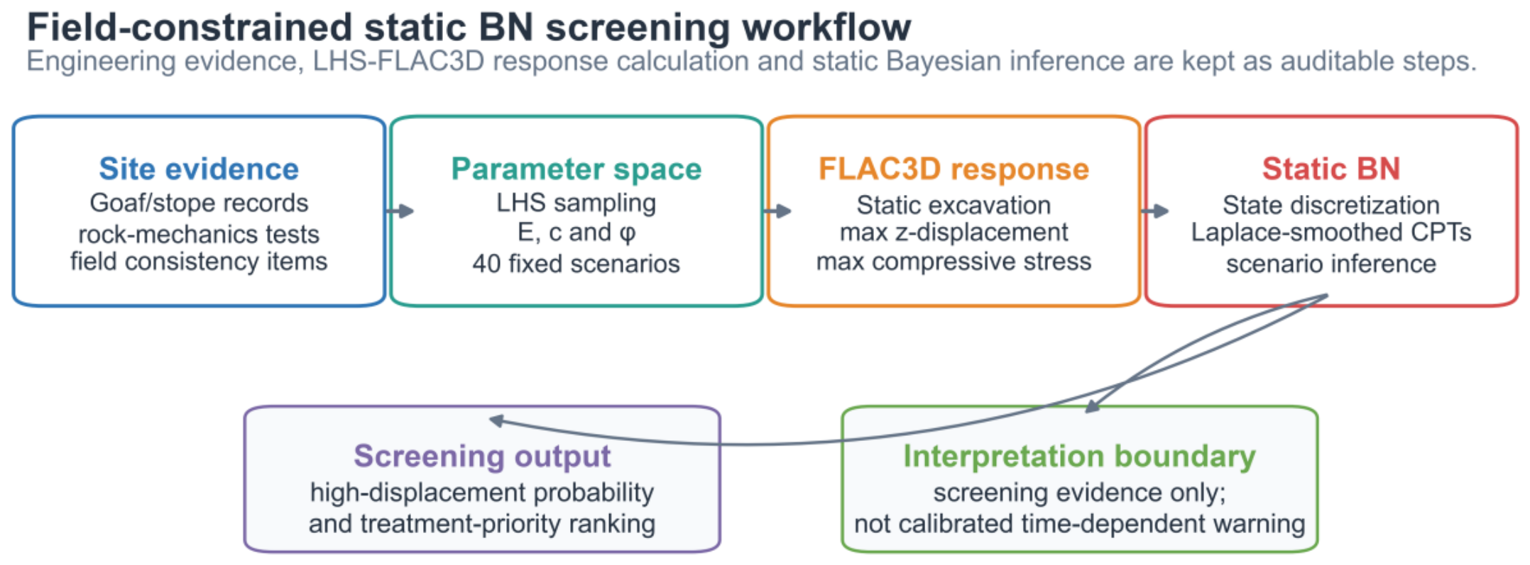
The primary objective is to test whether a field-constrained Latin hypercube sampling (LHS)-FLAC3D response library and static Bayesian inference can provide an auditable, uncertainty-aware screen of high-displacement scenarios in a data-sparse deep goaf group. The field inventory, laboratory evidence, numerical response audit, and probability interval analysis are successive steps toward this single objective.

Accordingly, the study does not estimate chain instability propagation. Goaf location and treatment state remain engineering context, not calibrated BN parent nodes. The reported probabilities refer only to the high-displacement screening state within the fixed numerical response library.

2. Materials and Methods

2.1. Study Area, Elevation Records, and Geometry Uncertainty

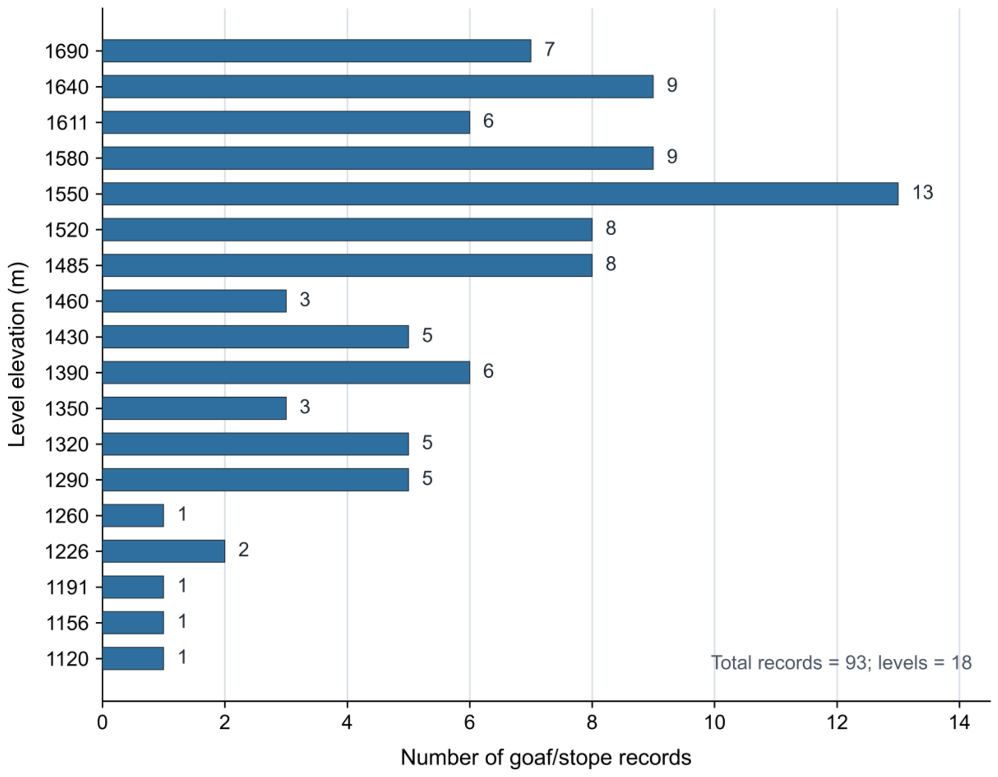
The engineering records list 93 goafs or active stopes on 18 mining levels labeled from 1120 m to 1690 m. These values are mine record-level elevations rather than burial depths. The engineering survey further states that the uppermost goafs lie approximately 100–200 m below the ground surface. Because the archived vertical datum is not documented, the level labels are not converted to elevations above sea level or used as point-specific cover depths. Recorded states include closure, natural collapse, partial collapse, engineered backfilling, waste rock backfilling, untreated openings, and active stopes (Figure 1).

Most historical goafs are sealed or unsafe to enter, and representative inaccessible or collapsed openings at the 1430 m and 1290 m levels were checked by drilling. Accessible voids were measured with a handheld laser rangefinder, whereas inaccessible geometries were reconstructed from mine records and envelope coordinates. This mixed provenance can bias span, roof thickness, void volume, separation, and apparent connectivity. Underestimated spans, excessive roof thicknesses, or oversized pillars would tend to suppress calculated deformation, whereas enlarged spans, reduced roof thicknesses, or artificially connected envelopes would tend to increase deformation and interaction. An illustrative ±5–10% perturbation cannot be reported as a quantitative sensitivity test because the retained archive does not identify defensible baseline spans and roof thicknesses for the modeled envelopes, nor does it preserve the geometry generation and zone mapping route needed to perturb them reproducibly. Applying arbitrary percentage changes to unidentified geometric quantities would introduce analyst-selected assumptions rather than quantify the uncertainty of the actual mine geometry. The impact of geometry uncertainty on maximum displacement is therefore assessed only by its expected direction, treated as model-form uncertainty, and excluded from the reported BN probabilities. All location-specific decisions require new survey confirmation before quantitative geometry sensitivity can be performed.

2.2. Available FLAC3D Model, Geometry, and Boundary Conditions

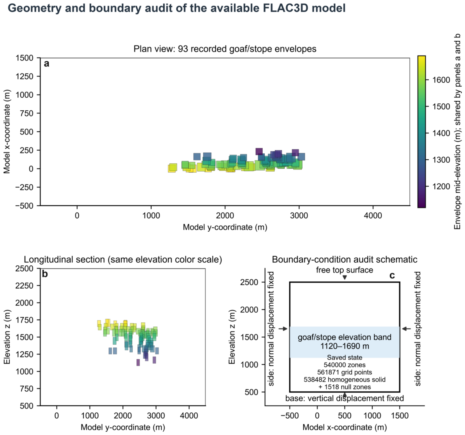
Figure 2 shows the available FLAC3D 7.00 saved model. The rectangular domain spans x = −500 to 1500 m, y = −500 to 4500 m, and z = 500 to 2500 m, giving overall dimensions of 2000 × 5000 × 2000 m. It contains 540,000 zones and 561,871 grid points. The saved state includes 1518 null zones. Reapplying the 93 goaf/stope envelopes marked 1528 zones, of which 1518 were already null and only 10 were solid. The lateral boundaries restrain normal displacement, the base restrains vertical displacement, and the top remains free. The calculation is quasi-static; inertial collapse, creep, and time-dependent degradation are not represented.

2.3. Laboratory Evidence and Engineering-Lithology Context

Core and block samples were inspected, oriented where possible, cored or cut into cylindrical and rectangular specimens, and ground at both ends. Diameter, height, and end-face quality were checked with a digital caliper before testing. Specimens were conditioned mainly in the saturated state; fault gouge and highly fractured mud-rich material that could not survive saturation or intact specimen preparation were tested in the natural state. Uniaxial compression and deformation measurements used a 1000 kN computer-controlled electro-hydraulic servo machine with strain and displacement instrumentation, while shear strength parameters were obtained with a rock direct shear apparatus. The archived report does not state the loading rate, stress control path, replicate-level failure mode, or uncertainty for every group, so those details are not inferred.

Specimens had diameters of 48–54 mm and height-to-diameter ratios of 2.0–2.5. Thirty-six sample groups were submitted, 248 specimens were prepared, 236 passed dimensional and appearance inspection, and 12 failed. Only 12 groups yielded complete mechanical index sets; the other 24 were limited by fragmentation, joints, insufficient block size, or water-sensitive disintegration. This is not random missingness: competent material is more likely to yield intact specimens, so the complete case subset may over-represent stronger, less fractured rock and under-represent weak tails. The rejected groups do not have complete, paired E, c, and φ values. Their joint parameter distribution, lower tail bounds, and correlations are therefore unidentified. Expanding the lower bounds by an arbitrary percentage would be a hypothetical stress test, not a quantitative estimate of complete-case selection bias. Consequently, the magnitude and direction of bias in the FLAC3D displacement distribution and BN probabilities cannot be calculated from the retained specimens. The laboratory results define engineering envelopes and lithological contrasts, not a site-wide probability distribution. LHS-BN probabilities remain conditional on the selected envelopes and must not be interpreted as population frequencies (

Table 1. Physical and mechanical parameters used to describe the engineering rock-mass classes of the Lehong Pb-Zn mine.

Rock Mass Zone	Compressive Strength (MPa)	E (GPa)	ν	c (MPa)	φ (°)
Ore body (pyrite-bearing carbonate rock)	47.06	14.80	0.22	2.11	47.6
Competent roof/surrounding rock (argillaceous dolomite)	91.30	31.20	0.22	4.06	52.3
Competent floor (dolomitic rock)	73.40	25.80	0.19	2.80	49.4
Weak layer/trigger source (fault gouge/fractured zone)	8.90	1.20	0.35	0.85	22.0

Note: For the weak layer/trigger source, uniaxial compressive strength (UCS) = 8.90 MPa is the report-derived mean natural compressive strength of fault-gouge/mylonitic fractured material. The E = 1.20 GPa, ν = 0.35, c = 0.85 MPa and φ = 22.0° values are conservative numerical-model inputs retained from the original FLAC3D parameter dataset rather than direct laboratory averages.

).

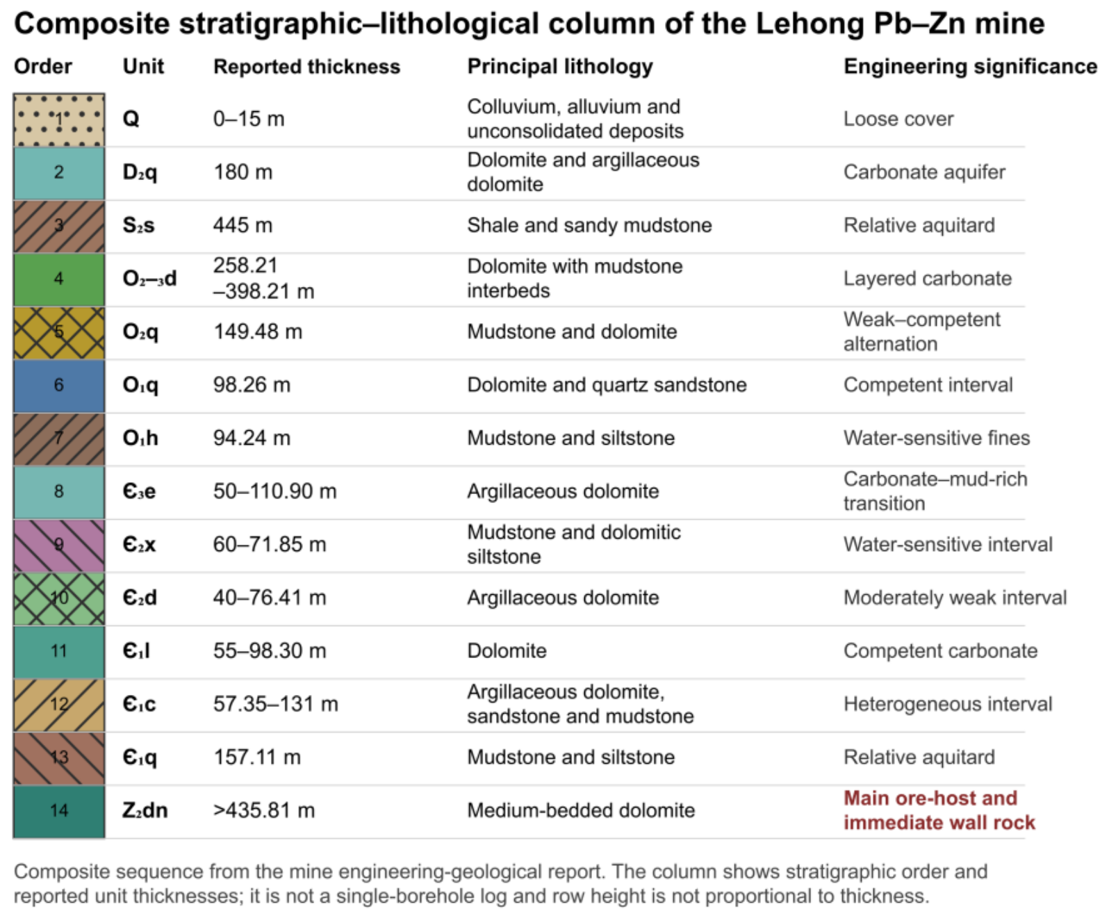
Figure 3 presents a composite mine-scale stratigraphic-lithological column compiled from the engineering–geological report. The principal sequence extends from Quaternary cover through Devonian, Silurian, Ordovician and Cambrian units to the upper Dengying Formation (Z2dn), a >435.81 m medium-bedded dolomite that forms the main ore host and immediate wall rock. Mudstone–, siltstone–, and argillaceous–dolomite intervals identify water-sensitive or relatively low-permeability contrasts relevant to parameter degradation. This is a composite regional column, not a single borehole log; row heights are not proportional to thickness, and the available FLAC3D save does not zone these units by depth.

At mine scale, the F1–F3 fault systems and associated gouge/fractured dolomite zones provide plausible pathways for localized weakening and water sensitivity. Their mapped existence is engineering evidence, whereas their three-dimensional continuity, aperture, and constitutive response are not resolved in the archived continuum model.

2.4. Evidence Sources and Evaluation Boundary

The evidence chain uses field records to define the goaf population and treatment context, laboratory evidence to constrain plausible parameter envelopes, FLAC3D to generate static mechanical responses, and the BN to compare discretized response scenarios. No continuous monitoring sequence is used. The Mathews assessment is retained only as a field-constrained consistency audit, not as a validation label for BN training (Figure 4).

2.5. LHS-FLAC3D Sampling and Bayesian Network Inference

The static BN contains E, c, and φ as mechanical parent nodes and the binary high-displacement screening state as the child node used in the principal probability analysis. Maximum compressive stress is retained as an archived FLAC3D output for descriptive comparison, but it is not a parent node and does not define the screening state. Goaf location, treatment state, adjacency, shared pillars, and structural connectivity are not encoded as BN parents because the retained inventory cannot support a calibrated spatial-coupling model. The BN therefore answers a parameter degradation screening question, not a transfer-of-instability question (

Table 2. Static Bayesian network nodes, state divisions, and evidence sources.

Node/Variable	Role in the Network	State Division	Threshold or Evidence Source
Mining level and treatment state	External engineering context (not a BN node)	Level, goaf identity and treatment state; applied only in post-BN site triage	Field investigation and goaf records
E	Mechanical parent node	Relatively intact/degraded	Median discretization of 40 LHS samples; range 10.09–21.40 GPa
c	Mechanical parent node	Relatively intact/degraded	Median discretization of 40 LHS samples; range 1.24–2.78 MPa
φ	Mechanical parent node	Relatively intact/degraded	Median discretization of 40 archived samples; range 37.75–55.00°
Maximum stress	Archived FLAC3D output; not a parent in the principal BN screen	Continuous response retained for descriptive comparison	Reported in the response library; no decision threshold assigned
Maximum vertical displacement	FLAC3D response used to define the BN child state	Continuous response recorded at Q75	Upper quartile of 15.04 cm defines high-displacement state
High-displacement screening state	Binary BN child node	No/yes	Mapped from displacement state; not equivalent to field failure frequency

).

For parent state combination g and binary child state s, the conditional probability is estimated as $\mathrm{P}\left(\mathrm{s}|\mathrm{g}\right)={\displaystyle \frac{{\mathrm{n}}_{\mathrm{g}\mathrm{s}}+1}{{\mathrm{n}}_{\mathrm{g}}+2}}$, which is equivalent to a Beta (1,1) prior and Laplace smoothing. Here, ${\mathrm{n}}_{\mathrm{g}\mathrm{s}}$ is the count in child state s and ${\mathrm{n}}_{\mathrm{g}}$ is the number of scenarios under g. Beta posterior 95% credible intervals are reported because several combinations contain few observations.

The three binary parents yield eight state combinations. The 40-scenario library gives unequal counts across these combinations. The resulting probabilities are conditional screening outputs from a designed numerical library, not observed field probabilities.

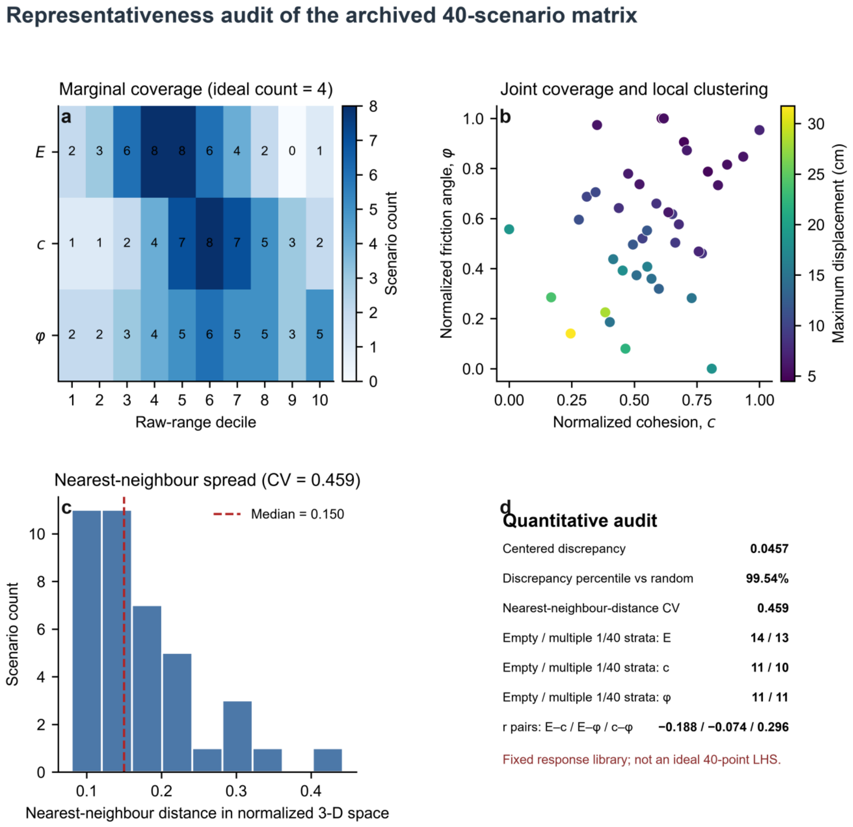
The original LHS seed, generating distributions, and permutation metadata were not recoverable; therefore, the archived 40-row matrix defines the analysis. Representativeness was audited in the normalized raw parameter range using decile occupancy, nominal 1/40-stratum occupancy, centered discrepancy, pairwise correlations, and nearest-neighbor distances. For E, c, and φ, respectively, 14, 11, and 11 nominal strata are empty, and 13, 10, and 11 are multiply occupied. The centered discrepancy is 0.04568 (99.54th percentile relative to 5000 random uniform reference designs; larger is less space-filling), and nearest-neighbor distance ranges from 0.0799 to 0.4423 with median 0.1500 and coefficient of variation 0.459. These diagnostics reveal marginal imbalance and local clustering; the matrix is retained as a fixed response library rather than claimed to be an ideal LHS. This audit is important because recent geotechnical applications use LHS to reduce deterministic computational demand while retaining explicit coverage of uncertain inputs [22]; that benefit depends on a recoverable and adequately space-filling design.

The sampled ranges are E = 10.09–21.40 GPa, c = 1.24–2.78 MPa, and φ = 37.75–55.00°. Maximum compressive stress ranges from 53.69 to 63.77 MPa, and maximum downward displacement ranges from 4.48 to 31.75 cm. The high-displacement screening state uses the response library Q75 value of 15.04045 cm. This threshold is a relative statistical screen and has no demonstrated equivalence to a regulatory limit, observed failure displacement, or evacuation criterion.

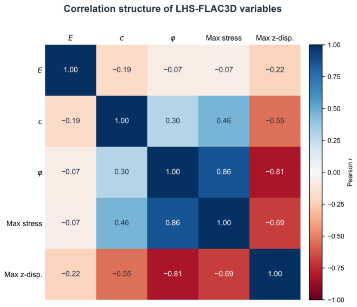
Empirical input correlations are r(E,c) = −0.188, r(E,φ) = −0.074, and r(c,φ) = 0.296. These departures from independence motivate standardized regression and partial correlation diagnostics.

2.6. Traceability Materials and Audit Boundary

The numerical and probabilistic audit trail consists of the fixed 40-row response matrix, explicit state definitions, the FLAC3D restoration and assignment route, posterior probability intervals, and representative reset runs. Mine drawings, full engineering reports, and saved numerical models contain controlled engineering information and are not presented as unrestricted public data (

Table 3. Traceability materials, manuscript locations, and access boundaries.

Traceability Item	Manuscript Location or Material Class	Purpose in Traceability/Audit	Access Boundary
LHS-FLAC3D response library	Reported in the full response library table in Section 3.1	Provides the 40 input–output scenarios used for descriptive statistics, displacement thresholding, and BN state recoding.	Included within the manuscript; no separate public data file is claimed.
BN node thresholds	Reported in Section 2.5 and the Bayesian network state definition table	Defines the E, c, φ, and high-displacement states used to construct the static BN.	Included within the manuscript.
Laplace-smoothed conditional probability tables (CPTs) and scenario probabilities	Defined in Section 2.5 and summarized in Section 3.3	Documents how sample frequencies were converted into initial static BN scenario probabilities.	Included within the manuscript as equations, thresholds, and scenario probability summaries.
Threshold and bootstrap checks	Reported in Section 3	Reports Q70/Q75/Q80 and fixed-threshold sensitivity, plus bootstrap stability of the correlation ranking.	Included within the manuscript as numerical summaries; no additional FLAC3D runs are implied.
FLAC3D calculation procedure	Described in the Methods and Figure 4 workflow	Documents model restoration, parameter assignment, goaf tagging, excavation nulling, solve criterion, and response extraction.	Mine-specific command files are treated as controlled audit materials and are not redistributed as public data.
Static BN model structure	Reported in Section 2.5 and Section 3.6	Documents node states, directed edges, and representative evidence propagation states.	The manuscript reports the model structure and inference summaries; any editable model file remains controlled.
Figure source values	Reported in manuscript tables and data-derived figures	Links plotted quantities to the reported 40-row response matrix and scenario summaries.	Source values needed to interpret the figures are included in the manuscript.
Saved initial numerical state	Described conceptually in the Methods	Provides the mine-specific equilibrium state from which the 40 static scenarios were restored.	Controlled mine-engineering audit material; not treated as public data.
Rock mechanics evidence audit	Reported in Table 1	Maps laboratory and engineering–geology facts used in Table 1 to the 2024 rock mechanics report.	The internal report is cited as an unpublished technical report; the manuscript reports the values used in the analysis.
Weak-zone parameter provenance	Reported in Table 1 and the Discussion	Separates laboratory-supported weak material evidence from conservative numerical model inputs.	The interpretation boundary is stated in the manuscript; no separate public provenance file is claimed.
Inventory Mathews record crosswalk	Supplementary Table S1	Maps all 93 inventory IDs to 186 roof/sidewall assessments and treatment context.	Crosswalk supplied; underlying mine reports remain controlled engineering records.
Additional FLAC3D sensitivity calculations	Section 3.4 and Section 3.5	Tests response reproducibility, deterministic E-c-φ co-degradation, and local hotspot mesh sensitivity.	Command logic and numerical results are reported; mine geometry and saved state remain controlled.

).

The BN state definitions are reported in

Table 4. Bayesian network node states and discretization thresholds.

Node	Variable	States	Threshold/Source	BN Role
E	Elastic modulus (GPa)	degraded < 14.80922; relatively intact ≥ 14.80922	Median of the 40 LHS samples	Parent node
c	Cohesion (MPa)	degraded < 2.10369; relatively intact ≥ 2.10369	Median of the 40 LHS samples	Parent node
φ	Friction angle (°)	degraded < 47.53178; relatively intact ≥ 47.53178	Median of the 40 LHS samples	Parent node
High displacement	Maximum vertical displacement (cm)	low < 15.04045; high ≥ 15.04045	Upper quartile of displacement response	Child response node

because discretization directly affects the static screening probabilities.

Each scenario restores the same saved initial state, assigns the row-specific E, c, and φ values to group Default = Brick1, applies the goaf/stope envelopes under slot Excavation, assigns the selected zones to the null model, solves the static response, and exports maximum downward displacement and maximum compressive stress. The saved model audit shows that Default = Brick1 contains all 538,482 solid zones. It is therefore one equivalent homogeneous continuum group, not a lithology-specific or depth-dependent material group. The initial saved values were approximately E = 31.19 GPa, ν = 0.220, c = 4.06 MPa, φ = 52.27°, and density = 2747–2752 $\mathrm{k}\mathrm{g}·{\mathrm{m}}^{-3}$.

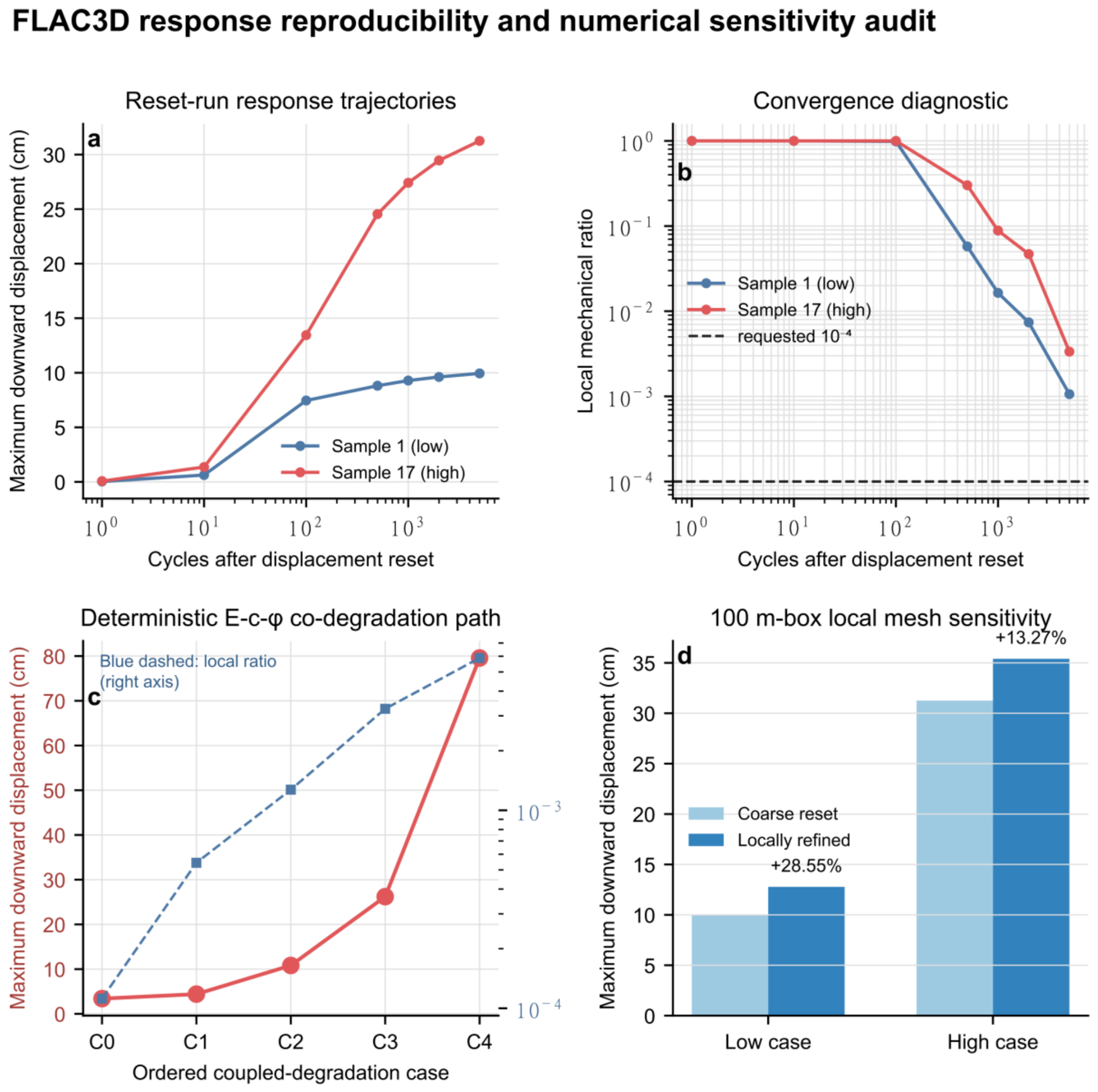
The archived batch command requests a local mechanical ratio of $1\times {10}^{-4}$, but the representative 5000-cycle audits reported in Section 3.4 remained above this target. The response library is therefore treated as archived fixed output; reset calculations are used only to assess response contrast and sensitivity, not to certify equilibrium.

All scenarios restore the same archived initial state, which records 28,360 completed cycles, before applying row-specific material parameters and excavation tags. This common restoration controls cross-scenario comparability, but the original gravity-loading sequence, tectonic stress assumptions, and any field in situ stress calibration are absent from the retained archive. The stored stress field is therefore an inherited numerical initial condition rather than a field-validated stress model. Lateral normal displacement is restrained, the base is fixed vertically, and the top is free; no inertial, creep, or dynamic subsidence calculation is performed.

The engineering–geological report identifies major F1, F2, and F3 faults and describes fault gouge, fractured dolomite, and broken zones. These observations justify the weak material envelope in Table 1, but the available data do not represent the mapped discontinuities as interfaces, ubiquitous joints, or explicit weak zone geometries, nor do they assign lithologies by depth. The model is therefore an equivalent homogeneous Mohr–Coulomb continuum; joint slip, fault-controlled localization, and structural connectivity are unresolved model-form uncertainties.

2.7. Decision Boundary of the Static BN

Table 5. Engineering decision boundary of the static Bayesian network screen.

Decision Class	Supported by the Present Static BN	Requires Dynamic Evidence
Risk management	Relative scenario screening; monitoring and inspection priority; treatment triage	Real-time warning; evacuation trigger; time-to-failure
Spatial interpretation	Use inventory as engineering context	Propagation direction; transition between individual goafs
Required evidence	Fixed numerical response library and explicit CPTs	Continuous displacement or microseismic records; repeated scanning/InSAR; treatment response sequences
Validation status	Field-constrained consistency audit	Out-of-sample temporal calibration and false alarm/missed alarm evaluation

separates decisions supported by the present static screen from decisions that require time series evidence and dynamic inference. The distinction is operational: a static probability may prioritize where to inspect or monitor, but it cannot define when a failure will occur.

3. Results

3.1. Parameter Space and Response Statistics

The fixed matrix spans E = 10.09–21.40 GPa, c = 1.24–2.78 MPa, φ = 37.75–55.00°, and maximum downward displacement = 4.48–31.75 cm. The raw range decile counts depart from four per bin; the centered discrepancy is 0.04568, and the nearest-neighbor distance coefficient of variation is 0.459. Figure 5 therefore documents the archived matrix’s non-ideal coverage and clustering rather than asserting ideal LHS uniformity (

Table 6. Descriptive statistics for the 40 LHS-FLAC3D samples.

Variable	Mean	Standard Deviation	Minimum	Maximum
E (GPa)	14.85	2.29	10.09	21.40
c (MPa)	2.10	0.32	1.24	2.78
φ (°)	47.48	4.50	37.75	55.00
Maximum stress (MPa)	57.27	4.20	53.69	63.77
Maximum vertical displacement (cm)	11.61	6.58	4.48	31.75

). The complete set of 40 LHS-FLAC3D scenarios is summarized in

Table 7. Full 40-row LHS-FLAC3D response library used for Bayesian network recoding and posterior probability calculation.

Sample	E (GPa)	c (MPa)	φ (°)	Max Stress (MPa)	Max z-Disp. (cm)
1	15.935702	1.720119	49.606513	56.4650	10.02860
2	10.932335	1.833458	41.639229	53.7756	28.26370
3	11.984697	1.939978	44.518285	53.7231	17.83910
4	11.482549	2.090810	44.783195	53.7111	16.36590
5	14.289728	2.579892	51.816122	63.4889	5.44195
6	12.965893	2.678584	52.363640	63.6150	5.90310
7	14.197554	1.774189	49.917902	57.9116	10.46200
8	16.783752	1.973751	51.190683	62.0575	6.40802
9	15.156598	2.425880	45.702936	53.6859	8.61277
10	12.810896	2.244109	48.409264	58.4306	9.13165
11	15.332398	1.244885	47.362027	53.7342	18.75740
12	18.158372	2.043161	50.464327	61.3865	6.03220
13	16.374537	2.061561	46.730009	53.6920	9.72726
14	10.094307	2.778031	54.198231	63.7739	7.31596
15	16.083773	2.485834	37.754567	53.7887	18.40330
16	16.986558	2.178358	55.000000	63.5147	4.48254
17	13.349244	1.621308	40.177721	53.8306	31.74830
18	16.595625	1.957084	39.132504	53.8137	21.99510
19	17.230992	1.671819	48.024976	53.6978	11.12000
20	17.840500	2.405742	45.831873	53.6854	7.35964
21	15.578093	2.315414	53.375525	63.4765	4.89449
22	14.926186	1.502087	42.671813	53.7893	23.92540
23	21.402904	1.861350	40.967383	53.7856	15.01300
24	13.247282	1.882183	45.301428	53.7170	15.68170
25	14.692251	1.783375	54.547354	63.1630	5.89803
26	13.695918	2.146570	49.133346	59.4088	8.44941
27	14.517718	2.002919	46.307120	53.6990	12.00910
28	12.575859	2.362841	42.618921	53.7218	15.12280
29	11.950885	2.333435	52.800725	63.4182	6.45313
30	18.685633	2.219990	48.533490	58.5483	6.26945
31	17.375903	1.916326	48.823768	56.4663	8.35944
32	15.392979	2.284245	47.701543	57.0313	7.93467
33	13.862162	2.191880	55.000000	63.5220	5.47057
34	14.004323	2.524132	50.397421	63.0250	5.84985
35	15.713320	2.161741	43.258242	53.7257	13.01730
36	15.069476	2.262315	46.438039	53.6861	9.09645
37	16.189373	2.462000	51.333871	63.2532	4.92138
38	13.581501	2.116574	43.953092	53.7194	14.40850
39	12.431400	2.089503	47.276433	54.0048	11.92110
40	14.583360	2.025061	44.193416	53.7217	14.21030

, providing the numerical basis for subsequent Bayesian network state recoding and posterior probability estimation. (Table 7). Figure 6 presents the correlation structure among the original LHS-FLAC3D variables, providing a visual overview of the pairwise relationships within the archived response library.

The table reports the fixed sample record used in this study. The original LHS seed was not recoverable; therefore, the numerical values below, rather than a regenerated pseudo-random sequence, define the sample set used for BN recoding.

3.2. Marginal and Conditional Parameter Effects

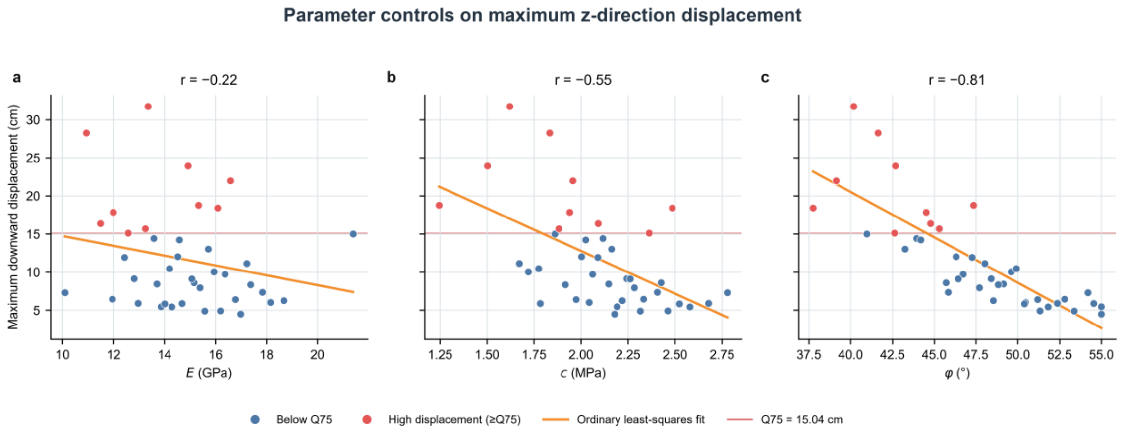
Marginal Pearson correlations with maximum downward displacement are r = −0.220 for E, −0.550 for c, and −0.810 for φ. Standardized multivariable coefficients are −0.354, −0.406, and −0.720, respectively, while partial correlations are −0.724, −0.755, and −0.901. Thus, φ remains the strongest effect within this response matrix, but the conditional E effect is materially larger than its marginal correlation alone suggests (Figure 7).

In 10,000 bootstrap resamples, median marginal correlations were −0.227 for E, −0.561 for c, and −0.821 for φ. The corresponding 95% percentile intervals were [−0.514, 0.086], [−0.719, −0.316], and [−0.880, −0.753]. The absolute marginal correlation ordering was retained in 96.1% of resamples. This is an internal diagnostic of the fixed matrix, not evidence that the same ordering holds under alternative geometries or correlated degradation processes.

The φ effect is physically consistent with the Mohr–Coulomb relation τ = c + σn tanφ. At high normal stress, reducing φ changes the stress-dependent frictional term, whereas c contributes an intercept and E primarily controls elastic stiffness. A lower φ can therefore promote wider shear yielding and larger deformation. However, the present analysis does not quantify plastic-zone connectivity, so this mechanism is interpreted as physically plausible rather than directly demonstrated.

3.3. Conditional Probability of the High-Displacement Screening State

The Q75 threshold of 15.04 cm identifies the upper quartile of the numerical response library. It is not a code-based stability limit, a measured failure threshold, or a site-wide safety criterion. Its purpose is to define a reproducible relative screening state for scenario comparison.

Threshold sensitivity was assessed with Q70, Q75, Q80, and fixed 10, 15, and 20 cm thresholds. The baseline probabilities were 0.31, 0.26, and 0.21 for Q70–Q80, while c + φ degradation gave 0.67, 0.60, and 0.53. For the fixed thresholds, baseline probabilities were 0.48, 0.29, and 0.12, compared with 0.87, 0.67, and 0.33 under c + φ degradation.

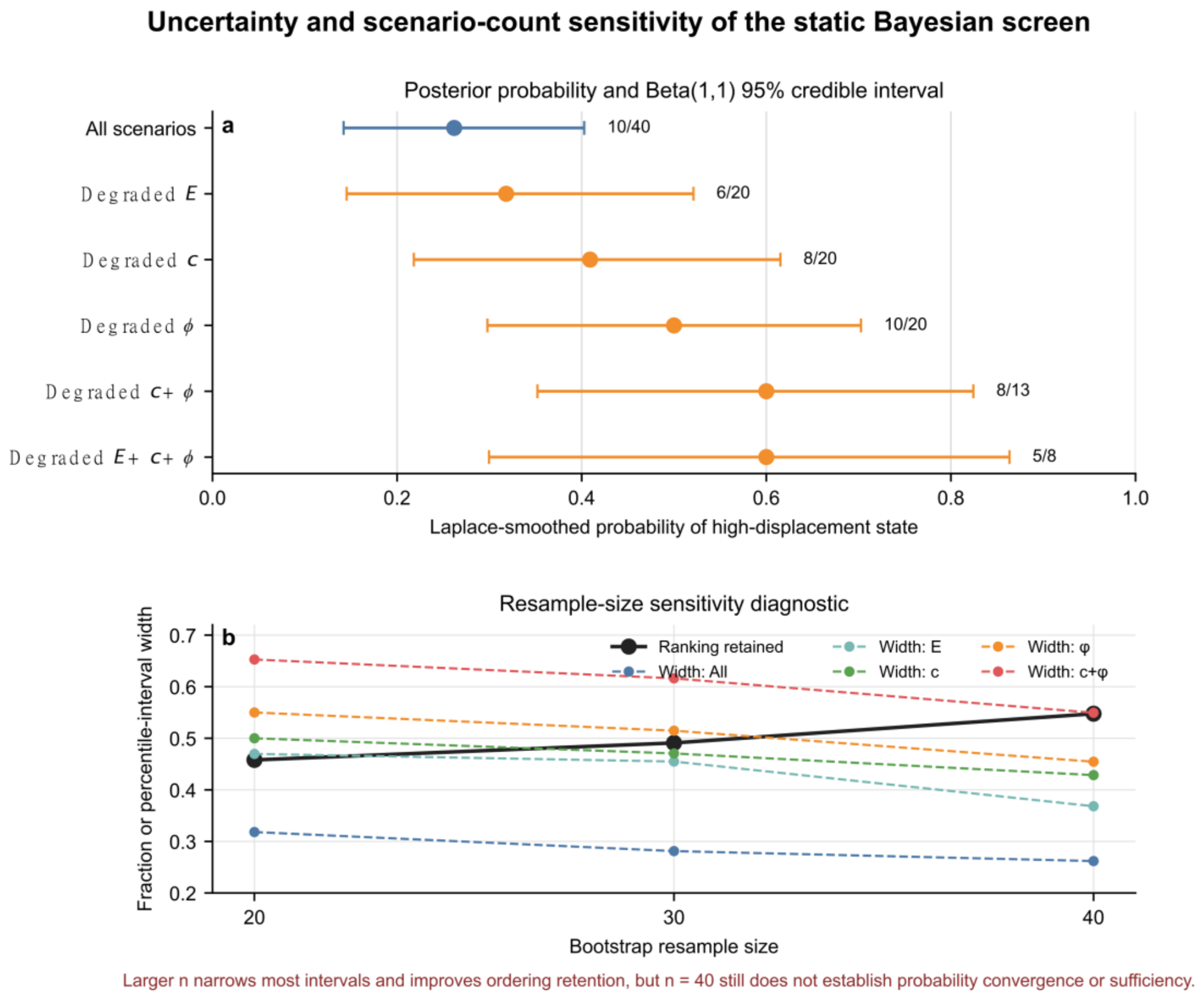
At Q75, the Laplace-smoothed point estimates increase from 0.262 for all scenarios to 0.600 for joint c + φ degradation. However, the Beta (1,1) 95% credible intervals overlap strongly. Bootstrap resampling retained the complete point-estimate ordering in 40.0% of replicates, or 54.5% when ties were accepted. The evidence supports an upward point estimate trend, not a robust complete ranking (Figure 8).

Scenario count sensitivity was evaluated with 10,000 bootstrap resamples of size n = 20, 30, and 40 drawn with replacement from the fixed 40-row library. The target scenario ordering was retained in 45.8%, 49.1% and 54.8% of replicates, respectively. For the baseline screen, the percentile interval width decreased from 0.318 at n = 20 to 0.281 at n = 30 and 0.262 at n = 40; the corresponding c-φ widths were 0.653, 0.616 and 0.549. Increasing n improves precision, but this retrospective down-sampling cannot demonstrate that 40 scenarios are sufficient or that probabilities have converged.

A record-level audit of the source tables identified 93 unique goaf IDs in the engineering inventory and the same 93 IDs in the Mathews table, with two exposed surfaces per goaf (186 surface records). No ID is unmatched. The raw goaf class labels contain 17 stable, 53 local risk, one ‘basically stable’, and 22 instability risk records; harmonizing ‘basically stable’ with the local risk class gives 17 stable, 54 basic/local risk, and 22 instability risk goafs. The source report’s nearby narrative total of 18 stable, 53 local risk, and 22 risk cases is therefore internally inconsistent with one detailed row. Supplementary Table S1 reports the record-level crosswalk, and the detailed table is treated as the auditable source.

Table 8. Field evidence and consistency-audit items used to constrain the Lehong goaf-group screening case.

Evidence Stream	Extracted Factual Item	Use in Manuscript	Boundary of Interpretation
Goaf inventory and elevation range	18 levels from 1120 to 1690 m; 93 goaf/stope records; statistics workbook reports 417,458.469 m3 of existing goaf volume.	Defines the case study population, level-wise inventory, and spatial scope for the FLAC3D/BN screening framework.	Used as engineering inventory evidence; not a continuous deformation or failure-time dataset.
Treatment and collapse state	The dominant recorded state is sealed and naturally collapsed goafs (57/93); other records include partial collapse, sealed-only, filling treatment, and active/untreated states.	Supports the manuscript statement that the goaf group contains mixed sealed, collapsed, and untreated openings.	State labels are used qualitatively because document versions use non-identical wording for treatment categories.
Field hazard context	The report describes two surface subsidence pits associated with goaf instability and notes that many goafs were not filled before sealing/natural collapse.	Justifies the need for group-scale risk screening rather than single-opening judgment.	This is hazard-context evidence, not a dated monitoring sequence for model calibration.
Drilling verification	Representative inaccessible or collapsed goafs at the 1430 m and 1290 m levels were checked by drilling to clarify internal conditions.	Supports the field-constrained interpretation of sealed/collapsed goaf conditions.	The manuscript does not infer displacement rates or failure probabilities from the drilling records.
Independent stability graph crosswalk	Detailed tables contain 93 unique goaf IDs and 186 exposed surfaces. Raw goaf labels: 17 stable, 53 local-risk, one basically stable, and 22 instability-risk; 93/93 IDs match the inventory.	Provides record-level engineering consistency and a transparent classification audit.	Not a displacement-monitoring validation dataset and not used as BN training labels.
Higher-priority worked case: 1520-2/1485-2	Active/untreated 1520-2 above sealed/collapsed 1485-2; nominal gap proxy 10 m. The lower goaf retains 9471.59 m3 and has a local risk roof plus an instability risk sidewall.	Priority survey, convergence monitoring and treatment review.	Engineering triage example; not validation of a goaf-specific BN probability.
Lower-priority worked case: 1640-2	Sealed/backfilled; 1447.10 m3 remaining; roof and sidewall stable.	Lower routine verification priority.	Requires current survey confirmation; not zero risk.

separates inventory facts, Mathews classifications, model outputs, and engineering decisions. The 93/93 crosswalk supports record-level consistency checking, but the Mathews classes remain independent engineering evidence rather than BN training labels or displacement monitoring validation.

Two worked cases demonstrate reproducible site-level triage. At overlapping section line intervals, active untreated 1520-2 (Mathews stable) lies above sealed, naturally collapsed 1485-2. Using the recorded mining levels as opening base elevations and the reported 25 m mean height of 1485-2 gives a reproducible nominal vertical gap proxy of 1520 − (1485 + 25) = 10 m. The lower opening has local risk roof status, instability risk sidewall status, and 9471.59 m³ remaining void volume; the combined evidence warrants priority survey, convergence monitoring, and treatment review even though 1520-2 alone plots as stable. By contrast, 1640-2 is sealed and backfilled, has stable roof and sidewall assessments, and retains 1447.10 m³; it is assigned lower routine verification priority. These examples do not prove BN prediction accuracy: they show how material scenario screening can be combined with inventory and Mathews evidence to form a transparent triage rule (Table 8).

This boundary allows the site materials to constrain plausibility and monitoring design without implying that the static BN predicts observed deformation rate, transition probability, or time-to-failure (

Table 9. Laplace-smoothed conditional probabilities with Beta (1,1) 95% credible intervals.

Scenario	High/n	Smoothed Probability	95% Credible Interval	Interpretation
All scenarios (baseline screen)	10/40	0.262	0.142–0.403	Reference
Degraded E	6/20	0.318	0.145–0.521	Point estimate
Degraded c	8/20	0.409	0.218–0.615	Point estimate
Degraded φ	10/20	0.500	0.298–0.703	Point estimate
Degraded c + φ	8/13	0.600	0.352–0.824	Wide interval
Degraded E + c + φ	5/8	0.600	0.300–0.863	Small n

).

3.4. Representative FLAC3D Response Consistency Audit

Displacement and velocity were reset before recalculating Sample 1 and Sample 17 for 5000 cycles. The incremental maximum downward displacements were 9.9417 cm and 31.2545 cm, compared with archived values of 10.0286 cm and 31.7483 cm; differences were 0.87% and 1.56%. Final local mechanical ratios were $1.061\times {10}^{-3}$ and $3.353\times {10}^{-3}$, above the requested $1\times {10}^{-4}$ target. A local 100 × 100 × 100 m box centered on the audited reset run displacement hotspot at (133.369, 2666.70, 1366.44) m was then densified by two segments in each direction and attached by face, creating 248 child zones and 99 attached grid points in each restored case. Sample1_low changed from 9.9417 to 12.7797 cm (+28.55%); Sample17_high changed from 31.2545 to 35.4027 cm (+13.27%). The low/high response ordering was preserved (refined high/low ratio = 2.77). This is a local mesh sensitivity check; it does not test a larger outer boundary or demonstrate full convergence (Figure 9).

3.5. Coupled E-c-φ Degradation Sensitivity

Along the five-case coupled degradation path, maximum downward displacement increased monotonically from 3.405 cm for the relatively intact combination to 79.577 cm for the lower envelope combination (+2237.3% relative to C0). The global maximum changed from (33.3, 1533.3, 1666.7) m in C0 to (133.4, 2667.1, 1365.8) m in C4 (separation 1177 m), with hotspot switching first evident in C2_midpoint. Because the cases are independent static restorations, this is scenario-dependent hotspot relocation, not evidence of temporal failure propagation. Each case restored the same saved state, reapplied the 93 excavation envelopes, reset displacement and velocity, and ran 5000 cycles. The path links the upper and lower parameter envelopes and therefore tests a plausible co-degradation direction; it does not estimate a natural joint distribution, isolate interaction terms, or replace a larger correlated design (

Table 10. Deterministic five-case coupled E-c-φ degradation sensitivity.

Case	E (GPa)	c (MPa)	φ (°)	Maximum Downward Displacement (cm)	Local Mechanical Ratio	Average Mechanical Ratio
C0_intact	21.403	2.778	55.000	3.4047	1.119 × 10−4	2.650 × 10−7
C1_mild	18.580	2.393	50.688	4.4087	5.432 × 10−4	1.322 × 10−6
C2_midpoint	15.749	2.011	46.377	10.8198	1.271 × 10−3	4.078 × 10−6
C3_severe	12.917	1.629	42.066	26.2056	3.256 × 10−3	9.692 × 10−6
C4_lower_envelope	10.094	1.245	37.755	79.5769	5.880 × 10−3	1.945 × 10−5

; Figure 9c).

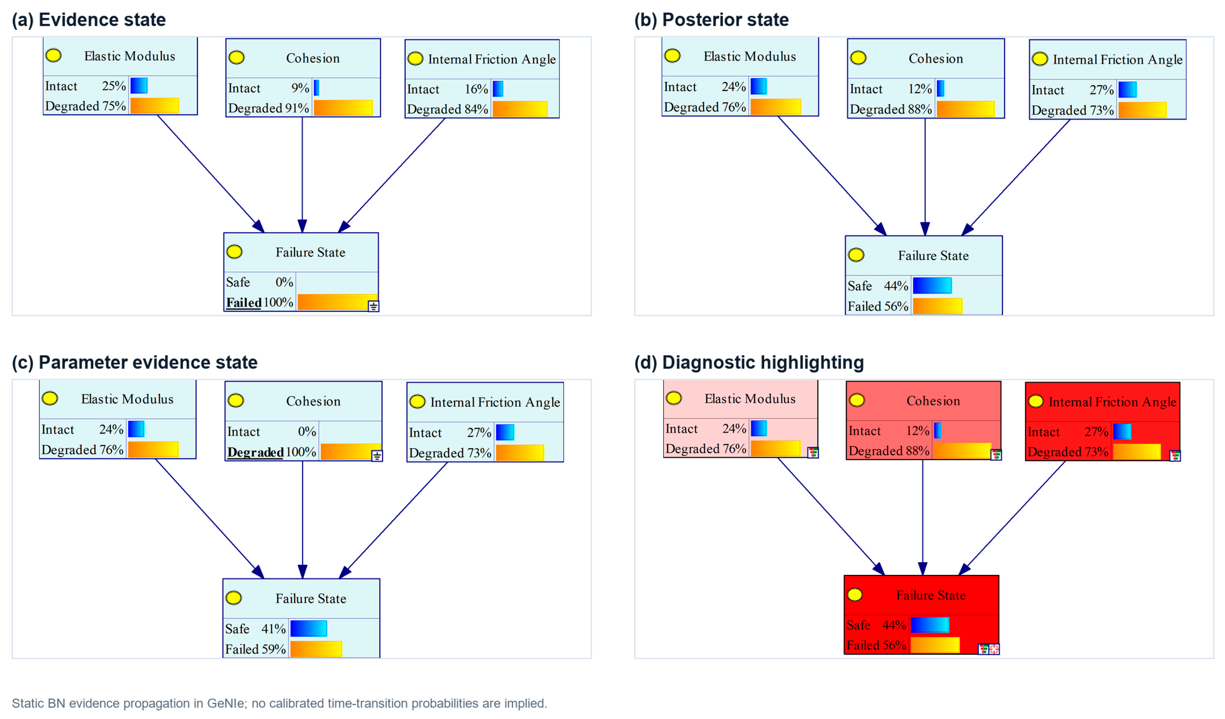
3.6. Static Bayesian Network Inference in GeNIe

The GeNIe model illustrates evidence entry, posterior updating, and reverse diagnosis within one static time slice. It does not contain temporal arcs or calibrated transition probabilities. Its outputs are therefore conditional screening probabilities tied to the state definitions in Table 4.

Figure 10 is retained as a software visualization of static evidence propagation. The GeNIe label “Failure State” maps to the manuscript’s high-displacement screening state and should not be interpreted as a calibrated probability of physical failure.

4. Discussion

The revised evidence supports high-displacement parameter screening rather than group-level collapse-propagation assessment. Within the fixed matrix, φ has the strongest marginal and conditional association with displacement (marginal r = −0.810; partial r = −0.901), followed by c. This ordering is physically consistent with the stress-dependent frictional term of the Mohr–Coulomb envelope, but it is conditional on one equivalent continuum geometry and the archived parameter ranges. Recent stope studies have generally evaluated prescribed geometries, excavation sequences, or exposure areas through deterministic numerical models [23,24,25,26,27,28]. In contrast, the present work samples E, c and φ jointly and quantifies both marginal and conditional effects. It therefore identifies parameter ranking uncertainty that a single deterministic design case cannot resolve, although it does not replace geometry-specific stability analysis.

The displacement response also differs in purpose from modern deterministic studies. The archived library spans 4.48–31.75 cm, and the illustrative five-case co-degradation path spans 3.405–79.577 cm. These values cannot be transferred as universal stability limits because mesh, geometry, stress field, constitutive assumptions, and response definitions differ among mines. Wang et al. used coupled 3D geological modeling and FLAC3D to locate roof and wall displacement around stopes beneath a subsidence area [23]. Huang et al. combined physical and numerical modeling for a tunnel beneath a coal seam goaf [24], while Lima et al. incorporated time-dependent deformation in stope analysis [25]. Recent creep-based analyses further demonstrate that backfilled stope stability depends on time as well as static material and geometry inputs [28,29]. You et al. used site-specific displacement bands of <20, 20–45, 45–100, and >100 mm to distinguish increasing levels of stope concern [27]. By comparison, the present response library range is 44.8–317.5 mm, and its Q75 screen is 150.4 mm, which illustrates why the threshold is a within-library ranking device rather than a transferable stability criterion. The present quasi-static library asks how uncertainty in selected material parameters changes relative displacement under one fixed archived geometry. Its contribution is a bounded scenario screen, not a claim that its displacement range is more accurate than those site-specific results.

Modern empirical–numerical studies also clarify the role of Mathews evidence. Cui et al. combined the Mathews stability chart with numerical analysis to optimize stope dimensions [26], and You et al. extended the stability graph with exposure time and FLAC3D analysis to select limit exposure areas [27]. These studies use empirical and numerical results directly in design optimization. The present 93/93 inventory Mathews crosswalk has a narrower function: it independently checks record identity and supports site-level triage, but it is not used as a BN training label. This separation avoids treating empirical classes as observed displacement outcomes while retaining them as field evidence.

The static BN alone prioritizes material scenarios, not named goafs. Site-level priority emerges only after the scenario evidence is combined with the external 93-record inventory, treatment status, spatial overlap, and Mathews classification, as illustrated by 1520-2/1485-2 versus 1640-2. This combined triage can guide confirmatory surveys, inspection frequency, monitoring installation, and treatment review, but it cannot provide real-time alarms, failure time, propagation direction, transfer probability, or evacuation thresholds. A dynamic extension requires synchronized displacement, microseismic, repeated scanning, or InSAR windows [30,31,32,33,34,35]; explicit t-to-t + 1 states; transition estimation; and held-out evaluation of false alarms and missed alarms.

The probabilistic layer likewise serves a different role from both a conventional stability calculation and a monitoring model. Mishra et al. showed that BNs can combine expert knowledge and accumulating underground mine data for geotechnical risk assessment [36]. Here, the BN is estimated only from 40 designed numerical scenarios, so it provides Laplace-smoothed conditional screening probabilities with wide credible intervals rather than field-calibrated roof fall or failure frequencies. Karatzetzou demonstrated the computational economy of LHS for uncertainty propagation through deterministic geotechnical software [22]. The current study adds an explicit audit showing that an archived sample labeled as LHS may be clustered and should not be assumed to have ideal space-filling properties. For operational validation, integrated D-InSAR, small baseline subset InSAR, and unmanned aerial vehicle monitoring can improve coverage and accuracy of mining subsidence observations [37]. Such time-resolved observations are absent at Lehong and are required before the static screen can be converted into a dynamic warning model.

A related application is underground coal gasification (UCG), where cavity adjacency and safety pillar condition can control overburden response. Sakhno et al. [38] used finite-element simulations for 30 m reactor cavities separated by pillars 3.75–15 m wide. For their site conditions, surface movement remained within the pre-peak response while pillar bearing capacity was maintained. Pillar destruction, by contrast, created a high risk of crack evolution in the overburden. The reported optimum pillar width was 15 m. This study supports the general importance of interaction geometry and treatment or pillar state, but it does not calibrate the present mine model. Direct transfer would require UCG-specific thermal, hydrological, lithological, and evolving cavity representations.

Several limitations remain. The 40 scenarios are insufficient for calibrated predictive probability: the resample size diagnostic narrows uncertainty but does not demonstrate convergence. Only 12 of 36 laboratory groups yielded complete indices, creating non-random complete case bias. Because the other 24 groups lack complete paired E, c, and φ values, neither their joint lower tail nor the resulting selection bias in FLAC3D and BN outputs can be quantified; arbitrary lower bound expansion would be hypothetical rather than data-derived. The archived LHS is clustered, and its generating metadata are unavailable. The retained archive also lacks defensible baseline spans, roof thicknesses, perturbable geometry mappings, and minimum/base/maximum envelopes. Therefore, no numerical ±5–10% geometry sensitivity result is claimed, and only the expected direction of bias is stated. The model has no explicit depth-dependent lithologies, faults, or joints, and the initial stress history cannot be reconstructed from field stress measurements. Representative reset and coupled degradation runs do not replace global mesh, boundary distance, or field monitoring validation. Although the 93/93 Mathews crosswalk and drilling checks strengthen engineering consistency, no continuous displacement time series is available.

These constraints define the proper engineering use of the framework. It is a traceable exploratory screen for comparing material degradation scenarios and planning additional monitoring. It is not a mine-wide failure probability, a chain-propagation model, a site-independent design rule, or an operational early warning system.

Future work should reconstruct the model from source geometry, define survey-supported baseline spans and roof thicknesses, and then conduct reproducible ±5–10% geometry perturbations. It should also test mesh and boundary distance, encode three-dimensional adjacency and treatment state, and obtain complete or alternative weak material measurements for the presently rejected sample groups. These data are required to quantify complete case selection bias instead of imposing arbitrary lower tail ranges. The scenario library should then be expanded through nested or incremental LHS, accompanied by continuous monitoring and treatment response records.

Only after those data are available should a time-indexed BN be calibrated and assessed for transition prediction, false alarms, and missed alarms.

5. Conclusions

(1) A field-constrained LHS-FLAC3D and static BN workflow was developed to screen high-displacement scenarios in the Lehong deep goaf group. The main contribution is an auditable evidence chain, not a calibrated chain instability probability.

(2) The available save spans 2000 × 5000 × 2000 m and contains 540,000 zones and 561,871 grid points. All 538,482 solid zones belong to one equivalent continuum group, Default = Brick1; lithology and discontinuities are not explicitly zoned.

(3) Within the fixed 40-scenario matrix, φ has the strongest marginal and conditional association with maximum downward displacement. Multivariable diagnostics show that the E effect is larger than the marginal r = −0.22 alone suggests. Along the five-case coupled degradation path, maximum downward displacement increased monotonically from 3.405 cm for the relatively intact combination to 79.577 cm for the lower-envelope combination (+2237.3% relative to C0). The global maximum changed from (33.3, 1533.3, 1666.7) m in C0 to (133.4, 2667.1, 1365.8) m in C4 (separation 1177 m), with hotspot switching first evident in C2_midpoint. Because the cases are independent static restorations, this is scenario-dependent hotspot relocation, not evidence of temporal failure propagation. This limited path does not define a joint probability distribution.

(4) At Q75 = 15.04 cm, the conditional probability increases from 0.262 for all scenarios to 0.600 for c-φ degradation, but the 95% credible intervals overlap widely. Bootstrap resampling retains the scenario ordering in only 45.8%, 49.1%, and 54.8% of replicates at resample sizes 20, 30, and 40, respectively; forty archived scenarios do not establish probability convergence.

(5) The 93/93 inventory Mathews crosswalk and contrasting 1520-2/1485-2 versus 1640-2 cases support transparent site-level triage when external engineering evidence is combined with BN material scenario results. The local mesh-refinement check quantifies whether the low/high displacement ordering is preserved, but larger boundary and continuous field monitoring validation remain outstanding. Quantitative ±5–10% geometry sensitivity and complete case selection bias estimates are not reported because the retained archive lacks perturbable geometry mappings and complete paired properties for the rejected groups. The corresponding effects are therefore stated as unresolved uncertainty rather than represented by invented numerical ranges.