An Induced Seismicity Indicator Using Accumulated Microearthquakes’ Frictional Energy

Abstract

Induced seismicity resulting from mining activities is one of the major challenges faced by the mining industry. Although such events have been documented for over a century in countries with extensive mining traditions, such as Canada, Australia, and Chile, their impact has intensified over time. This increase is primarily attributed to the greater extraction depths, where elevated stress levels and environmental conditions heighten the likelihood of rockburst occurrences. Seismic events within mines lead to significant human casualties and substantial infrastructure damage, necessitating the implementation of various safety protocols. Among these, seismic indicators are employed to identify periods when high-magnitude seismic events are most likely to occur through the analysis of parameters such as magnitude, energy, time, and decay rate. In this context, the present study aims to utilize the accumulated frictional energy generated by microearthquakes within the Bobrek mine, Poland, as a seismic indicator (variation of frictional energy in time), establishing its correlation with the occurrence of high-magnitude seismic events exceeding the background activity. Thousands of combinations of seismic parameters were tested to maximize the performance of this frictional energy-based indicator, parameters such as moment magnitude, frictional energy, and rock properties. The optimal set of parameters was determined using the Piece Skill Score (PSS) and subsequently applied to the Accumulated Frictional Heat (AFH) methodology. According to the results, the seismic indicator forecasts 86.6% of events with magnitudes M_w ≥ 2.3, with an average forecasting time of 9.76 h, indicating that, on average, these events can be anticipated approximately 10 h before their occurrence.

1. Introduction

Seismic events, occurring as a response of the rock mass to blasting and mining activities, can result in significant loss of human lives and severe infrastructure damage. Over the years, this issue has worsened due to the increasing depths of mineral extraction, where elevated stress levels and environmental conditions heighten the likelihood of rockburst occurrences. Small- and large-scale, as well as local or regional seismic events can add extra stress to the rock mass, triggering rockbursts [1,2]. Studies that involve field monitoring have shown that low energy events (<100 kJ) do not cause alteration in the rock. However, energetic events (>1.5 GJ) will cause rockbursts in all cases [3]. In general, rockbursts occur after seismic events [1,2], which facilitates the distinction between both rock mass reactions [2]. The common understanding regarding rockbursts occurrence is a dynamic rock failure, where static strain energy is converted to fracture and kinetic energies during bursting [2].

Rockburst cases have been documented in many countries, such as South Africa, the United States, Canada, Australia, and Chile [4,5]. In Chile, according to the Servicio Nacional de Geología y Minería SERNAGEOMIN (Geological and Mining National Survey), nearly 600 hundred fatal accidents occurred between 2000 and 2019 [6,7]. To deal with this problem, it is necessary to implement effective safety protocols, which are constantly improved and reassessed. Regarding this, one of the main goals of the mining industry is to be able to forecast at least mine-related seismic events with the best possible accuracy.

During an earthquake, the total energy released into the surrounding medium can be described based on fault parameters and the stresses acting on the fault plane, specifically shear stress and stress drop, both of which can be directly estimated from seismograms [8]. The static stress drop (Δσ_s) represents the difference between the initial and final stress states (σ₀ and σ₁), corresponding to the conditions before and after the earthquake (Figure 1a). Similarly, during fault sliding, the applied stress equals the frictional stress (σ_f (u)), which varies throughout the faulting process (Figure 1a). However, in the simplest model, frictional stress is assumed to remain constant and is defined as the average frictional stress during motion [9]. In this model, concerning earthquake energy distribution, potential energy is converted into elastic wave energy (E_R) and non-radiated energy (E_NR), with the latter consisting of fracture energy (E_G), required for mechanical weakening of the fault, and frictional heating energy (E_H), which is dissipated locally within the fault core [7]. A well-documented relationship exists between the thermal energy released during an earthquake (E_H), its effects on the fault plane, and the resulting temperature distribution in the surrounding area [10,11,12]. Estimating the frictional energy requires calculating the localized temperature increase in a narrow zone around the fault plane (Figure 1b). The rapid heating that occurs during co-seismic slip can weaken the rock and induce thermally driven fracturing by reducing friction [11,12,13]. However, these effects are not directly observable in seismograms, and most conclusions on the topic are based on theoretical models or experimental studies [10,11,14].

Over the last few decades, several seismic indicators have been developed to monitor the condition and response of the rock mass and the related seismicity [16,17,18,19]. This monitoring seeks to generate alert states in defined time windows, in which a major seismic event is probable to occur. In general, they are based on temporal and spatial clustering and probabilistic methods [19,20], which have, as a main objective, to provide an accurate definition of the seismicity decay rate behavior. Seismic indicators based on the energy of earthquakes have also been proposed. An indicator based on the cumulative total seismic energy normalized by the corresponding total within a defined time was presented by Hudyma et al. (2003) [21]. This method analyzes mainly structurally related seismicity, where large magnitude earthquakes may appear several days after a mine blast [20,21]. This seismic indicator allows re-entry when 90% of the energy is dissipated. A second approach, called instability analysis, was suggested by Mendecki et al. (1999) [22]. The instability analysis assumes that an energy index based on the seismic moment is directly related to stress distribution in the rock mass. Among other methodologies, we can additionally mention (i) the time variation of the Gutenberg–Richter b-value [23]. This technique identifies the periods with low b-value, which have a good correlation with the occurrence of high-magnitude seismic events [18,24,25,26], (ii) the time–magnitude plot that allows the estimation of the mechanism of seismic events, relating them to the variation in the stress field due to blasting or structural faults [27], (iii) the Es/Ep ratio, which compares the ratio between the energy of S and P waves, allowing to infer the type of rupture mechanism of the events [27], (iv) the temporal variation of the apparent stress, in which its higher values correlate with events of larger magnitudes [27], and (v) Mendecki (2023) [28], who defined the Ground Motion Alerts for Mines (GMAP), which use the behavior of the Peak Ground Velocity (PGV) and the Cumulative Absolute Displacement (CAD) to identify alert states through the GMAP ratings.

This study proposes a novel seismic indicator based on the earthquake frictional energy released by low- to intermediate-magnitude events. As a case study, we used open data of seismic events recorded during the years 2009–2010 in the Bobrek mine, located in Poland. We analyze the efficiency of the indicator using the Accumulated Frictional Heat (AFH) methodology. Results are examined using the ROC curve and the PSS statistical techniques. This method, which implicitly incorporates fault plane thermal processes, attempts to move the seismic indicators one step ahead from the purely probabilistic approaches. Additionally, it seeks to complement the results presented by previously published earthquake energy-based seismic indicators [21,22].

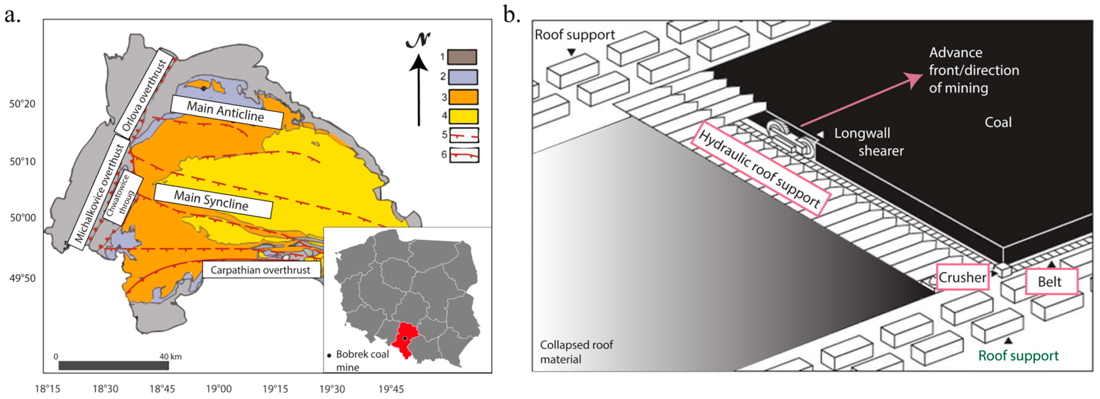
2. Geological Setting

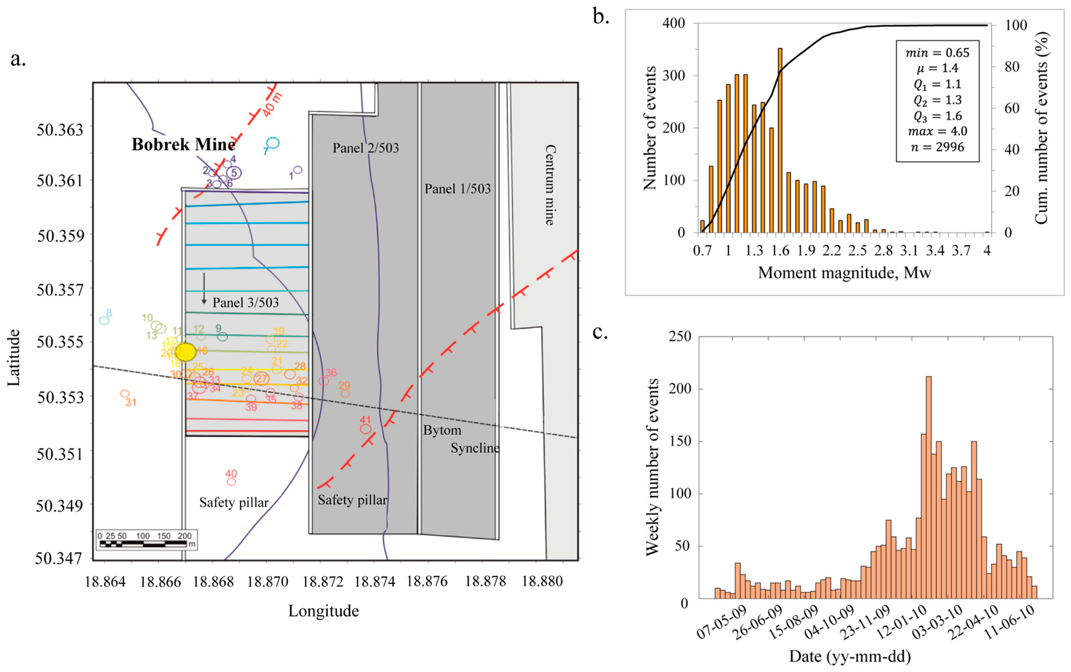
The Bobrek mine is located in the Upper Silesian Coal Basin (USCB) in Poland (Figure 2a). The USCB is one of the most seismically active mining areas in the world, registering around 56,000 mining tremors with local magnitudes over 1.5 during the period 1975–2005 [23]. In the USCB, two different types of tremors have been identified. The first kind is mining tectonic seismicity, which arises from the interaction between tectonic structures and mining activity. This kind of seismic event is more energetic, and source mechanisms are mostly normal dip-slip faults with a noticeable strike-slip component. The second type is mining seismicity, which is directly associated with mining activity and is mostly located in the vicinity of active excavations. These events are less energetic, and the source mechanism is explosive [23].

The USCB coal deposits are distributed in four lithostratigraphic series of the Carboniferous age (Figure 2a). The coal-bearing Carboniferous sequence from the Mississippian to Pennsylvanian Series has different compositions. The Mississippian Series are composed of clastic and phytogenic rocks plus marine fauna, where coal seams appear as thin layers. The Pennsylvanian Series are predominantly composed of sandstones, conglomerates, and coal-bearing rocks with fine-grained sediments. Coal seams range from thin to thick and are variable and numerous, reaching up to ~9% of the profile for the Lower Pennsylvanian age [24]. The Carboniferous sequence is covered by Permian, Triassic, and Jurassic rocks—clastics, calcareous-dolomites, and limestones—to the east and north of the basin. On the other hand, a thick Miocene sequence composed of clays, conglomerates, and claystones cover its central and southern parts [24].

Several tectonic structures can be found in this area; however, only three of them directly influence the Bobrek mine: the Bytom Syncline Complex, the Main Anticline Complex, and the Klodniki Fault Zone (Figure 2b) [29]. The Bytom Syncline is the closest structure and is composed of sedimentary rocks interspersed with coal layers [30].

The exploitation is based on the longwall system, extracting the coal using a shearer, which is moved laterally and forward between the headgate and tailgate galleries. The process leaves behind collapsed roof material (Figure 2b) in a cavity called goaf.

Figure 2. (a) Bobrek mine location in the USCB, Poland [30,31] with the lithostratigraphic and tectonic units of the USCB. In the legend, from 1 to 4: Paralic Series, Upper Silesian Sandstone Series, Mudstone Series, Krakow Sandstones Series. Numbers 5 and 6 indicate the path of primary faults and overthrusts [30]. (b) Schematic representation of the longwall coal mining method [32].

Figure 2. (a) Bobrek mine location in the USCB, Poland [30,31] with the lithostratigraphic and tectonic units of the USCB. In the legend, from 1 to 4: Paralic Series, Upper Silesian Sandstone Series, Mudstone Series, Krakow Sandstones Series. Numbers 5 and 6 indicate the path of primary faults and overthrusts [30]. (b) Schematic representation of the longwall coal mining method [32].

3. Data

For this study, we used an earthquake catalog composed of 2996 seismic events recorded between the years 2009 and 2010 in panel number 3, vein 503 (Figure 3a) [31]. The depth of the panel is 700 m below the surface. After 16 December 2009, the activity significantly increased by 18 events per day approximately, due to the occurrence of an M_w = 4.0 earthquake (Figure 3b,c) 750 m below the active front of the longwall panel, which was related to the proximity between the Bytom Syncline and the longwall face advancement (Figure 3a) [33]. The seismic events were recorded by a local network installed inside the mine and constituted originally by 13 vertical and five triaxial seismographs [34]. The dataset was downloaded from the European Plate Observing System (EPOS) webpage [31].

4. Methodology

As a starting point, we calculate the thermal energy released by seismic events. This energy depends on faulting parameters, rock properties, moment magnitude, and seismic stress drops. Once the thermal energy is calculated, we proceed with the construction of several sets of seismic parameters, which test the efficiency of the seismic indicator via the Accumulated Frictional Heat (AFH) method. Its performance is further estimated using the Receiver Operating Characteristic analysis (ROC) and the maximization of the Pierce Skill Score (PSS) metric.

4.1. Earthquake’s Frictional Energy

The total heat, $Q$ generated during faulting can be calculated using the faulting area, S, the displacement offset, $D$, and the frictional stress, ${\sigma }_f$ as:

$$Q={\sigma }_{f}DS$$

(1)

If the heat is distributed within a layer of thickness $w$ around the rupture plane, the average temperature rise can be expressed in terms of the specific heat, C, and the density, ρ, as:

$$∆T={\displaystyle \frac{Q}{C\rho Sw}}={\displaystyle \frac{{\sigma }_{f}D}{C\rho w}}$$

(2)

Using a simplified circular model [10,36], and considering the static stress drop, $∆{\sigma }_S$, the rigidity, μ, and the seismic moment, $M_0$, the displacement offset, $D$, can be written as:

$$D={\left({\displaystyle \frac{16}{7}}\right)}^{2/3}{\displaystyle \frac{1}{\pi \mathsf{\mu }}} {∆{\sigma }_S}^{2/3}{M_0}^{1/3}$$

(3)

Then, the temperature rise defined in Kanamori & Heaton (2000) [10] is obtained by combining Equations (2) and (3):

$$∆T={\left({\displaystyle \frac{16}{7}}\right)}^{2/3}{\displaystyle \frac{1}{\pi \mathsf{\mu }C\rho w}}{\sigma }_f {∆{\sigma }_S}^{2/3}{M_0}^{1/3}$$

(4)

where the seismic moment is related to $M_W$ through

$$\log M_0=1.5 M_w+9.1$$

(5)

Grünthal et al. (2009) [37] proposed a relationship to convert between local ($M_L$) and moment ($M_w$) magnitudes for small earthquakes (0 ≤ M_L ≤ 3.8):

$$M_w=0.906M_L+0.65$$

(6)

To calculate the total heat generated during faulting, it is necessary to reuse Equation (1). By considering the static stress-drop calculated from $D$ (Equation (3)) and the fault dimension through $S$ and $C_s$ [32], it can be stated that

$$∆{\sigma }_S=C_S\mathsf{\mu }D/S^{1/2}$$

(7)

If $M_0=\mathsf{\mu }DS$, then

$$M_0=C_S∆{\sigma }_S{S}^{3/2}$$

(8)

where $C_S\approx 1$ [38,39]. Finally, the total heat produced by a single event can be obtained by combining Equations (1), (3) and (8):

$$Q={\displaystyle \frac{{\sigma }_f}{\pi \mathsf{\mu }}}{\left({\displaystyle \frac{16}{7}}\right)}^{{\displaystyle \frac{2}{3}}}\mathsf{\Delta }{\sigma }_s s^{{\displaystyle \frac{3}{2}}}$$

(9)

The selection of rock parameters was based on the main observed lithology close to the Bobrek mine, where sandstones are dominant [40]. In addition, $\mathsf{\Delta }{\sigma }_s$ and ${\sigma }_f$ were obtained from previous data of induced mining events [41] (

Table 1. Values of rock parameters considered in the calculation of the seismic frictional heat.

Parameter	Range of Values for Sandstones
C (J/kg K)	787–915 [42]
ρ (kg/m3)	2000–2760 [43]
μ (GPA)	4–30 [44]
ΔσS (MPA)	0.1–10 [41]
σF (MPA)	14.9–20 (considering an initial tectonic stress between 15 and 30 MPa [45])
w (m)	0.001–0.01 [10]

).

4.2. Accumulated Frictional Heat (AFH)

The AFH methodology seeks to determine the two parameters critical accumulated heat (Q*) and critical moment magnitude (Mw*), which allow the best performance of the seismic indicator. The critical moment magnitude indicates the minimum magnitude from which a seismic event is considered relevant for the seismic indicator. In the same way, the critical accumulated heat establishes the minimum amount of heat over which it is possible to initiate an alarm state for the occurrence of a seismic event with magnitude M ≥ Mw*, in the next Δt_f = 24 h (Figure 4a). Choosing this time enables the incorporation of a greater amount of seismicity in the analysis, given the low seismicity rate of the mine (6.6 events/day). It also coincides with a time that can be associated with short-term decisions in case of a state of alert.

From the previous analysis, four different cases are possible:

• Q > Q*: An alert state is defined. If during the next Δt_f hours a seismic event with magnitude M ≥ Mw* occurs, this is classified as a True Positive (TP).
• Q > Q*: An alert state is defined. If during the next Δt_f hours a seismic event with magnitude M ≥ Mw* does not occur, this is classified as a False Positive (FP).
• Q < Q*: No alert state is defined. If during the next Δt_f hours a seismic event with magnitude M ≥ Mw* occurs, this is classified as a False Negative (FN).
• Q < Q*: No alert state is defined. If during the next Δt_f hours a seismic event with magnitude M ≥ Mw* does not occur, this is classified as a True Negative (TN).

4.3. Performance Analysis

Receiver Operating Characteristic (ROC) analysis is a common graphical technique used to visualize, organize, and select different kinds of classifiers based on their efficiency [46]. This method has been extensively applied to analyze seismic indicators [17,18,47]. The ROC analysis can have four different outcomes: True Positive (TP), False Positive (FP), True Negative (TN), and False Negative (FN), which can be expressed in a confusion matrix. The ROC space can also be visualized by plotting the True Positive Rate (TPR) vs. the False Positive Rate (FPR) (Equations (10) and (11)), where TPR indicates the percentage of high-magnitude events occurring during an alert state and FPR is defined by the percentage of false alarms.

$$TPR={\displaystyle \frac{TP}{TP+FN}}$$

(10)

$$FPR={\displaystyle \frac{FP}{FP+TN}}$$

(11)

In this representation, a classifier has a 100% sensitivity (no false negatives) and a 100% specificity (no false positives) when data are clustering into the upper left corner [46]. A 100% accuracy indicator then satisfies TPR = 1 and FPR = 0.

Another statistical index is the Peirce Skill Score (PSS) [48] (Equation (12)) which is based on the difference between the TPR and the FPR. This difference indicates the indicator forecasting performance, with a perfect, random, or bad classification model, with results equal to 1, 0, or −1, respectively [48].

$$PSS=TPR-FPR$$

(12)

4.4. PSS Maximization Procedure

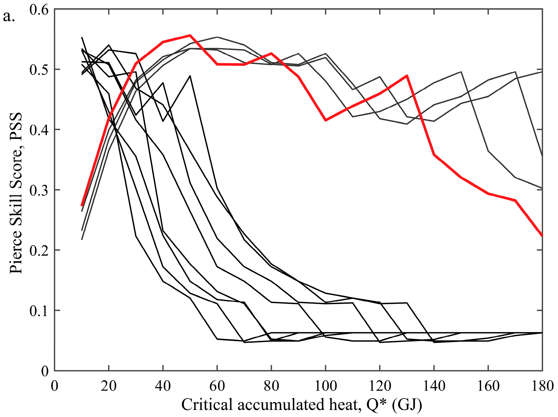
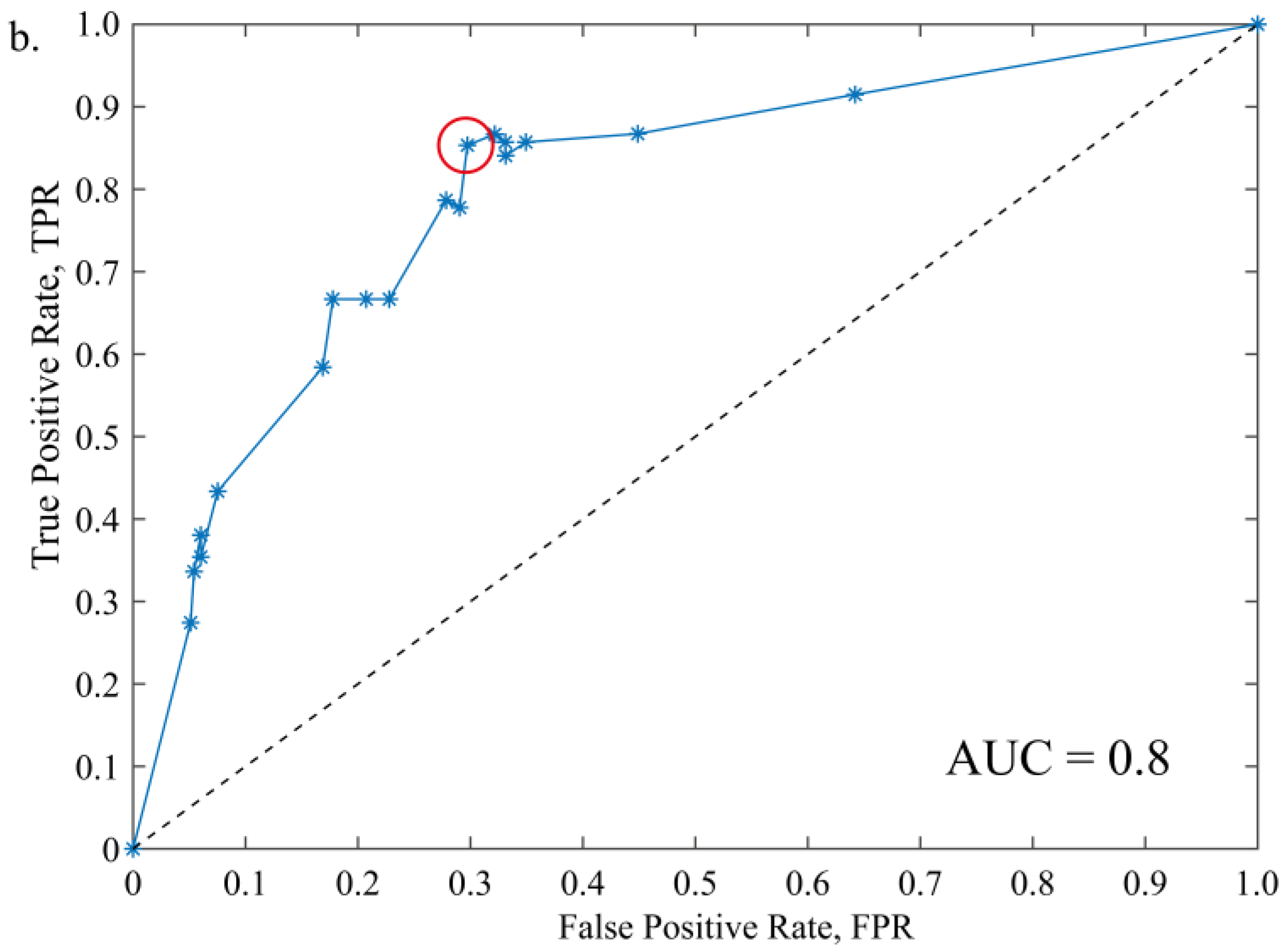
The main uncertainties of the proposed seismic indicator are the variability during the selection of the rock parameters shown in Table 1 and the election of the critical values of Q* and Mw*. To overcome this issue, we searched for a combination of parameters that maximize the PSS value. The total number of steps used and the total quantity of values per parameter are shown in

Table 2. Total number of Steps and Quantities per parameter used during calculation. Steps are the space between selected values (Table 1), creating the Quantity, which indicates the number of different parameters to be used during the calculation of the seismic indicator. In this way, 2880 combinations have been generated. For example, for the specific heat, C (Table 1), three different values (787, 837, and 887 J/kg K) have been used. Each combination was tested, changing the values of Q* and Mw*.

Parameter	Steps	Quantity
C (J/kg K)	50	3
ρ (Kg/m3)	200	4
μ (GPa)	10	3
ΔσS (MPa)	4	4
σF (MPa)	2	4
w (m)	0.002	5
Q* (GJ)	10	18
Mw*	0.1	16

. In total, 2880 combinations were performed.

Each curve in Figure 4a corresponds to different sets of parameters (Table 1 and Table 2), representing the variation of PSS vs. Q*. By testing all combinations (Table 2), the PSS reaches a maximum value of 0.56 (Figure 4) when Q* = 50 GJ and M * = 2.3, which is shown in the red curves (Figure 4a). This maximum value for PSS was found for 240 different combinations. For simplicity, only one of these combinations was selected to estimate the seismic indicator. The combination used for the final calculation was Δσ_s = 0.1 MPa, σ_f = 14.9 MPa, w = 0.001 m, c = 787 J/kg K, ρ = 2000 kg/m³, and μ = 4 GPa.

Figure 4. (a) Peirce Skill Score variations for different values of Q*. Red color curves are those reaching the maximum value of PSS, equal to 0.56. Black color curves are included for comparative purposes and show the value of PSS for different sets of parameters. (b) ROC curve for the best-case scenario combination, where the maximum value of PSS is indicated with the red circle. The dashed line corresponds to the bisector line of the graph.

Figure 4. (a) Peirce Skill Score variations for different values of Q*. Red color curves are those reaching the maximum value of PSS, equal to 0.56. Black color curves are included for comparative purposes and show the value of PSS for different sets of parameters. (b) ROC curve for the best-case scenario combination, where the maximum value of PSS is indicated with the red circle. The dashed line corresponds to the bisector line of the graph.

Figure 4b shows the ROC matrix for all possible combinations. The red circle shows the set of combinations with the maximum PSS value. The Area Under the Curve (AUC) indicates the probability that the classifier will rank a randomly chosen positive instance higher than a randomly chosen negative instance [46]. For example, in Figure 4b, there is an 80% chance that the indicator will correctly forecast the occurrence of a seismic event with magnitude M_w ≥ 2.3 after reaching the state alert, instead of such an event not occurring.

5. Results

Once the heat energy released by each seismic event is estimated (Equation (9)), we calculate the AFH indicator considering the abovementioned parameters, which maximize the PSS value. Figure 5a shows the seismic indicator performance. All events with magnitude $M_w\ge 2.3$ are shown with black triangles. Of those, events forecasted by the seismic indicator are marked with red triangles. Events with magnitudes $M_w\ge 3.0$ are represented with green triangles, and forecasted events with magnitudes over 3.0 are shown with green color–red border triangles (Figure 5a).

According to the results, the seismic indicator forecasts 86.6% of events with magnitudes $M_w\ge 2.3$, with an average forecasting time of 9.76 h, which means that events are, on average, anticipated approximately 10 h before their occurrence (Figure 5d). Regarding a total of six earthquakes with magnitudes $M_w\ge 3.0$ present during the study period, the seismic indicator is in an alert state during 83.3% of the cases. This high forecasting percentage is related to the indicator efficiency, which reaches 56% through the PSS estimation.

6. Discussions and Conclusions

The presented results were obtained considering a specific regional context, where the surrounding rock properties highly influence the frictional energy values (Equations (1)–(9)). In the same way, for these calculations, we have used a reference stress drop for mining tremors obtained from Abercrombie and Leary (1993) [41]. Although these stress values seem to be representative, the outcomes of this study might be improved by calculating the stress drop and the frictional stress values using local seismic activity. Considering its high dependency on the local context, the AFH method should be replicated in different geological and mining environments, for example, in highly tectonically active regions. This would allow us to analyze its efficiency under other geographical constraints with a different calibration of the parameters used.

The parameters involved in energy estimation and the correct real-time application of the seismic indicator strongly depend on how well the seismic signal was recorded and processed [17,49]. In this way, the seismic network configuration and its recording sensitivity are extremely prominent issues [50]. The use of a seismic network uniquely composed of triaxial equipment might improve the signal quality. This would benefit the assessment of seismic parameters, for example, the earthquake magnitude.

The frequency and magnitude distribution of seismic events (Figure 3b,c) are typical of mining conditions, and they result from a combination of mining and mining-tectonic activity. A priori, we believe that the longwall extraction is an optimal mining method for the application and testing of the AFH approach, as seismic events occur with a temporal and spatial correlation with the face advancement (Figure 3a). The nature of the longwall method with minimum use of blasting contributes to this fact, as the induced seismicity location is mainly related to the extraction processes. Regarding forecasting, this also constitutes an advantage since it is most likely that the location of high-magnitude events will follow this spatial delimitation. This behavior is different from other extraction techniques, for example, the caving method at the El Teniente mine in Chile, where seismicity has a heterogeneous distribution.

According to the results, the AFH methodology seems to be effective in initiating an alert state approximately 10 h before a seismic event occurs. It is also worth noting that several combinations of parameters show the same PSS curves (Figure 4a), so the results might be affected by considering a different set with another value of Q*.

As lower-magnitude events were sometimes also categorized as potential high-risk earthquakes, this technique might be improved using an extended catalog, which offers more possibilities regarding different time-average windows.

Several combinations of the seismic parameters that maximize the PSS value were tested to explore the indicator performance. The largest variation in the performance was found when the frictional stress and the shear parameters were increasing their values, as the PSS was 0.56 when $\mathsf{\mu }$= 4 Gpa and $\sigma f =$14.9 MPa. In all cases with maximum PSS, the detection percentage remains constant at 86.6%.

The effects of frictional energy on the rock mass are being, for mining purposes, just recently explored. The method presented here opens several possibilities and questions. For example, how does the temperature increase and friction drop contribute to nucleate new events? What would the magnitude distribution be in such a case? Other seismic indicators related to the energy of earthquakes present similarities to our method [21,22]. For instance, the procedure proposed by Mendecki et al. (1999) [22] can be used to forecast medium-magnitude events based on cumulative energy. The approach is also highly dependent on the rock type. Regarding Hudyma’s routine, his results are time-dependent, which, in our case, is an issue that could be solved through the analysis of the PSS index. Finally, Hudyma et al. (2003) [21] suggested re-entry when 90% of the seismic energy was released. For the AFH method presented here, this constitutes a difficult point to analyze, as the residual effects of the friction decay at the fault plane and the stability decreasing remain unclear.

The main challenge in the application of the seismic indicator is related to the possibility of having a proper micro-seismic network in the mine for the acquisition of high-quality seismic data for the correct estimation of the seismic source parameters and the real-time calculation of the seismic indicator.

Regarding the abovementioned, as future work, we propose:

(i)

Attempt to empirically define the AFH method decay rate in order to be able to propose a re-entry protocol.

(ii)

Consider the relative spatial distance between events, as heat accumulation and transfer strongly depend on how the earthquakes are distributed.

(iii)

Seismicity monitoring and forecasting are topics of large concern in different contexts, such as geothermal and CO₂ injection [51,52]. In general, the most-used monitoring technique is Probabilistic Seismic Hazard Analysis (PSHA) [53]. To our knowledge, the application of probabilistic approaches such as the one presented in this study and others [21,22] is not an extended practice. Due to this, we plan to apply the AFH method to new datasets considering fracturing behavior induced by fluid injection.

(iv)

In consideration of the abovementioned seismic network functioning, a real-time monitoring test is planned for the AFH methodology.

In summary, this study has presented a novel seismic indicator that allows one to forecast high-magnitude mining seismic events. This is done by considering the temperature rise on a narrow zone of the fault plane and the subsequent accumulated frictional heat produced during their occurrence. Thousands of sets of seismic parameters were tested, looking for the best indicator performance. According to the results, the seismic indicator forecasts 86.6% of events with magnitudes over 2.3, with an average forecasting time of 9.76 h, which means that events are, on average, anticipated approximately 10 h before their occurrence.

This method is an alternative to the abovementioned traditional methods. In this study, we prioritize the optimization of the indicator parameters through the maximization of the PSS value. On the other hand, a future time is considered to evaluate the performance of the seismic indicator.

References

1. Kaiser, P.K.; McCreath, D.R.; Tannant, D.D.; Brummer, R.K.; Vasek, M.; Yi, X.P. Rockburst support-volume 2 of rockburst research handbook. In Canadian Rockburst Research Program 1990–1995; CAMIRO Mining Division: Sudbury, ON, Canada, 1996. [Google Scholar]
2. Li, C.C.; Mikula, P.; Simser, B.; Hebblewhite, B.; Joughin, W.; Feng, X.; Xu, N. Discussions on rockburst and dynamic ground support in deep mines. J. Rock Mech. Geotech. Eng. 2019, 11, 1110–1118. [Google Scholar] [CrossRef]
3. Salamon, M.D.G. Rockburst hazard and the fight for its alleviation in South African gold mines. In Rockbursts-Prediction and Control; Institute of Mines and Metallurgy: London, UK, 1983; pp. 11–36. [Google Scholar]
4. Gibowicz, S.; Kijko, A. An Introduction to Mine Seismology; Academic press: San Diego, CA, USA, 1994. [Google Scholar]
5. Potvin, Y.; Hadjigeorgiou, J.; Stacey, T.R.; Potvin, Y. Challenges in Deep and High Stress Mining; Australian Centre for Geomechanics: Perth, Australia, 2007. [Google Scholar]
6. Sernageomin. Balance Nacional de Accidentabilidad Minera de 2016. Available online: https://www.sernageomin.cl/accidentabilidad-minera/ (accessed on 26 February 2023). (In Spanish).
7. Sernageomin. Accidentabilidad Minera año 2019. Available online: https://www.sernageomin.cl/accidentabilidad-minera/ (accessed on 26 February 2023).
8. Stein, S.; Wyssession, M. Introduction to Seismology, Earthquakes and Earth Structure; Blackwell science Ltd.: Hoboken, NJ, USA, 2002. [Google Scholar]
9. Kanamori, H. Energy Budget of Earthquakes and Seismic Efficiency. In Earthquake Thermodynamics and Phase Transformations in the Earth’s Interior; International Geophysics Series 76; Academic Press: San Diego, CA, USA, 2001. [Google Scholar]
10. Kanamori, H.; Heaton, T. Microscopic and macroscopic physics of earthquakes. In Geocomplexity and the Physics of Earthquakes; Rundle, J.B., Turcotte, D.L., Klein, W., Eds.; Geophysical Mono-Graph Series 120; AGU: Washington, DC, USA, 2000. [Google Scholar]
11. Di Toro, G.; Han, R.; Hirose, T.; De Paola, N.; Nielsen, S.; Mizoguchi, K.; Ferri, F.; Cocco, M.; Shimamoto, T. Fault lubrication during earthquakes. Nature 2011, 471, 494–498. [Google Scholar] [CrossRef]
12. Aubry, J.; Passelègue, F.X.; Deldicque, D.; Girault, F.; Marty, S.; Lahfid, A.; Bhat, H.S.; Escartin, J.; Schubnel, A. Frictional heating processes and energy budget during laboratory earthquakes. Geophys. Res. Lett. 2018, 45, 12274–12282. [Google Scholar] [CrossRef]
13. Byerlee, J. Friction of rocks. Pure Appl. Geophys. 1978, 116, 615–626. [Google Scholar] [CrossRef]
14. Kanamori, H.; Rivera, L. Energy Partitioning During an Earthquake. In Earthquakes: Radiated Energy and the Physics of Faulting; Abercrombie, R., McGarr, A., Di Toro, G., Kanamori, H., Eds.; Geophysical Monograph Series 170; American Geophysical Union: Washington, DC, USA, 2006. [Google Scholar]
15. Pavez, C.; Estay, R.; Brönner, M.; Ortiz, A.; Debarbieri, F.; Ibañez, J.P.; Guzmán, L. Frictional energy patterns related to the temperature increases due to intraplate seismicity, southern Norway, 2000–2019 catalogue. Nor. J. Geol. 2021, 101, 202105. [Google Scholar] [CrossRef]
16. Ogata, Y. Statistical models for earthquake occurrences and residual analysis for point. J. Am. Stat. Assoc. 1988, 83, 9–27. [Google Scholar] [CrossRef]
17. Vallejos, J.; Estay, R.; Zepeda, R.; Jorquiera, P. A methodology for evaluating the performance of seismic indicators at El Teniente Mine, Chile. In Proceedings of the 6th International Conference & Exhibition on Mass Mining, Massmin, Sudbury, ON, Canada, 10–14 June 2012. [Google Scholar]
18. Estay, R. Metodología para la Evaluación del Desempeño de Indicadores Sísmicos en Sismicidad Inducida por la Minería. Master’s Thesis, Universidad de Chile, Santiago, Chile, 2014. (In Spanish). [Google Scholar]
19. Vergara, M. Evaluación del Desempeño del Indicador de Agloramiento Espacial Con Datos de Sismicidad Inducida por Minería. Bachelor’s Thesis, Universidad Técnica Federico Santa María, Santiago, Chile, 2021. (In Spanish). [Google Scholar]
20. Vallejos, J.A. Analysis of Seismicity in Mines and Development of Re-Entry Protocols. Ph.D. Thesis, Queen’s University, Kingston, ON, Canada, 2010. [Google Scholar]
21. Hudyma, M.; Heal, D.; Mikula, P. Seismic monitoring in mines–Old technology, new applications. In Seismic Monitoring in Mines-Old Technology, New Applications; Hebblewhite, B.K., Ed.; University of New South Wales School of Mining Engineering: Sydney, NSW, Australia, 2003. [Google Scholar]
22. Mendecki, A.; van Aswegen, G.; Mountfort, P. A guide to routine seismic monitoring in mines. In A Handbook on Rock Engineering Practices for Tabular Hard Rock Mines; Jager, A.J., Ryder, J.A., Eds.; Creda Communications: Cape Town, South Africa, 1999. [Google Scholar]
23. Gutenberg, B.; Richter, C.F. Seismicity of the Earth. Geol. Soc. Am. Bull. 1945, 56, 603–667. [Google Scholar] [CrossRef]
24. Holub, K. Spasce-time variations of the frequency-energy relation for mining induced seismicity in the Ostrava-Karviná mining district. Pure Appl. Geophys. 1996, 146, 265–280. [Google Scholar] [CrossRef]
25. Ma, X.; Westman, E.; Slaker, B.; Thibodeau, D.; Counter, D. The b-value evolution of mining-induced seismicity and mainshock occurrences at hard-rock mines. Int. J. Rock Mech. Min. Sci. Géoméch. Abstr. 2018, 104, 64–70. [Google Scholar] [CrossRef]
26. Mukuhira, Y.; Fehler, M.C.; Bjarkason, E.K.; Ito, T.; Asanuma, H. On the b-value dependency of injection-induced seismicity on geomechanical parameters. Int. J. Rock Mech. Min. Sci. Géoméch. Abstr. 2024, 174, 105631. [Google Scholar] [CrossRef]
27. Hudyma, M. Applied mine seismology concepts and techniques. In Technical Notes for ENGR 5356–Mine Seismic Monitoring Systems 2010; Laurentian University: Sudbury, ON, Canada, 2010. [Google Scholar] [CrossRef]
28. Mendecki, A. Seismic ground motion alerts for mines. J. Seism. 2023, 27, 599–608. [Google Scholar] [CrossRef]
29. Stec, K. Characteristics of seismic activity of the Upper Silesian Coal Basin in Poland. Geophys. J. Int. 2007, 168, 757–768. [Google Scholar] [CrossRef]
30. Kędzior, S. Methane contents and coal-rank variability in the Upper Silesian Coal Basin, Poland. Int. J. Coal Geol. 2015, 139, 152–164. [Google Scholar] [CrossRef]
31. IS EPOS Episode: Bobrek. Available online: https://tcs.ah-epos.eu/#episode:BOBREK (accessed on 26 February 2023).
32. Saki, S.A. Gob Ventilation Borehole Design and Performance Optimization for Longwall Coal Mining Using Computational Fluid Dynamics. Ph.D. Thesis, Colorado School of Mines, Golden, CO, USA, 2016. [Google Scholar]
33. Leptokaropoulos, K.; Staszek, M.; Cielesta, S.; Urban, P.; Olszewska, D.; Lizurek, G. Time-dependent seismic hazard in Bobrek coal mine, Poland, assuming different magnitude distribution estimations. Acta Geophys. 2017, 65, 493–505. [Google Scholar] [CrossRef]
34. Kozlowska, M.; Orlecka-Sikora, B. Assessment of Quantitative Aftershock Productivity Potential in Mining-Induced Seismicity. Pure Appl. Geophys. 2016, 174, 925–936. [Google Scholar] [CrossRef]
35. Mendecki, M.J.; Szczygiel, J.; Lizurek, G.; Teper, L. Mining-triggered seismicity governed by a fold hinge zone: The Upper Silesian Coal Basin, Poland. Eng. Geol. 2020, 274, 105728. [Google Scholar] [CrossRef]
36. Eshelby, J.D. The determination of the elastic field of an ellipsoidal inclusion and related problems. Proc. R. Soc. London. Ser. A. Math. Phys. Sci. 1957, 241, 376–396. [Google Scholar] [CrossRef]
37. Grünthal, G.; Wahlström, R.; Stromeyer, D. The unified catalogue of earthquakes in central, northern, and northwestern Europe (CENEC)-updated and expanded to the last millennium. J. Seism. 2009, 13, 517–541. [Google Scholar] [CrossRef]
38. Madariaga, R. Implications of stress drop models of earthquakes from the inversion of stress drop from seismic observations. Pure Appl. Geophys. 1977, 115, 301–316. [Google Scholar] [CrossRef]
39. Kanamori, H.; Anderson, D. Theoretical basis of some empirical relations in seismology. Bull. Seismo. Soc. Am. 1975, 65, 1073–1095. [Google Scholar] [CrossRef]
40. Mendecki, M.J.; Wojtecki, Ł.; Zuberek, W.M. Case Studies of Seismic Energy Release Ahead of Underground Coal Mining Before Strong Tremors. Pure Appl. Geophys. 2019, 176, 3487–3508. [Google Scholar] [CrossRef]
41. Abercrombie, R.; Leary, P. Source parameters of small earthquakes recorded at 2.5 km depth, Cajon Pass, southern California: Implications for earthquake scaling. Geophys. Res. Lett. 1993, 20, 1511–1514. [Google Scholar] [CrossRef]
42. Xiong, J.; Lin, H.; Ding, H.; Pei, H.; Rong, C.; Liao, W. Investigation on thermal property parameters characteristics of rocks and its influence factors. Nat. Gas Ind. B 2020, 7, 298–308. [Google Scholar]
43. Schön, J. (Ed.) Chapter 4—Density. In Developments in Petroleum Science; Elsevier: Amsterdam, The Netherlands, 2015; Volume 65, pp. 109–118. [Google Scholar]
44. Weijermars, R. Principles of Rock Mechanics; Alboran Science Publications: Amsterdam, The Netherlands, 1997; p. 359. [Google Scholar]
45. Jarosinski, M. Recent tectonic stress field investigations in Poland: A state of the art. Geol. Q. 2006, 50, 303–321. [Google Scholar]
46. Fawcett, T. An introduction to ROC analysis. Pattern Recogn. Lett. 2006, 27, 861–874. [Google Scholar] [CrossRef]
47. Toksanbayev, N.; Adoko, A.C. Predicting rockburst damage scale in seismically active mines using a classifier ensemble approach. IOP Conferr. Ser. Earth Environ. Sci. 2023, 1124, 012102. [Google Scholar] [CrossRef]
48. Peirce, C.S. The numerical measure of the success of predictions. Science 1884, 4, 453–454. [Google Scholar] [CrossRef]
49. Mendecki, A. Real time quantitative seismology in mines. In Rockburst and Seismicity in Mines, Proceedings of the 3rd International Symposium, Kingston, ON, Canada, 16–18 August 1993; Young, R.P., Ed.; CRC Press: Boca Raton, FL, USA, 1993. [Google Scholar]
50. Havskov, J.; Ottemöller, L.; Trnkoczy, A.; Bormann, P. Seismic Networks. In New Manual of Seismological Observatory Practice 2 (NMSOP-2); Bormann, P., Ed.; Deutsches GeoForschungsZentrum (GFZ): Potsdam, Germany, 2012. [Google Scholar]
51. Zhou, W.; Lanza, F.; Grigoratos, I.; Schultz, R.; Cousse, J.; Trutnevyte, E.; Muntendam-Bos, A.; Wiemer, S. Managing induced seismicity risks from enhanced geothermal systems: A good practice guideline. Rev. Geophys. 2024, 62, e2024RG000849. [Google Scholar] [CrossRef]
52. Cheng, Y.; Liu, W.; Xu, T.; Zhang, Y.; Zhang, X.; Xing, Y.; Feng, B.; Xia, Y. Seismicity induced by geological CO2 storage: A review. Earth-Sci. Rev. 2023, 239, 104369. [Google Scholar] [CrossRef]
53. Baker, J.W. Introduction to Probabilistic Seismic Hazard Analysis. In White Paper Version 2.1; Cambridge University Press: Cambridge, UK, 2015; p. 77. [Google Scholar]
Figure 1. (a) A schematic representation of a simplified stress release model for an earthquake. The light purple, purple, and green sections correspond to fracture energy (EG), radiated energy (ER), and thermal energy (EH). The frictional stress, σf(u) = σf, is defined as the average frictional stress, where u represents the slip along the fault plane. The displacement offset is denoted by D along the slip axis. The illustration provides insights into the behavior of the stress drop. (b) A schematic fault model depicting the heated zone, represented by the thickness (w) where thermal energy is dissipated [15].
Mining 05 00027 g001
Figure 3. (a) Schematic representation of Panel 3, vein 503. Colored circles represent seismic events, the yellow circle being the largest event (Mw = 4.0, December 2009). Colored lines show the correspondence between the longwall advance and the location of earthquakes. Red dashed lines indicate faults [35] (Modified from Mendecki et al., 2020). (b) Distribution of seismic events per day, where it is possible to observe an increase in seismic activity after December 2009. (c). Histogram showing the cumulative number of events vs. magnitude and its statistics during the years 2009–2010.
Mining 05 00027 g003
Figure 5. (a) Final seismic indicator considering the seismic parameters that maximize the PSS value. Q* is shown with a horizontal orange line. Triangle colors are organized as follows: black are all events with magnitude Mw  2.3, red are events detected by the indicator, and green are seismic events with Mw  3. (b) and (c) Zoomed areas, indicated with dashed red boxes in Figure 5a, showing in detail the periods with seismic events with magnitudes Mw ≥ 3. (d) Histogram showing the number of detected events with magnitude Mw ≥ 2.3 vs. the number of hours in which the indicator first reaches the alert state before the occurrence of a seismic event.
Mining 05 00027 g005