Abstract
Geotechnical complexity in mining often leads to geotechnical uncertainty which impacts both safety and productivity. However, as mining progresses, particularly for strip mining operations, a body of knowledge is acquired which reduces this uncertainty and can potentially be used by mining engineers to improve the prediction of future mining conditions. In this paper, we describe a new method to support this approach based on modelling and neural networks. A high-level causal model of the mining operations based on historical data for a number of parameters was constructed which accounted for parameter interactions, including hydrogeological conditions, weather, and prior operations. An artificial neural network was then trained on this historical data, including production data. The network can then be used to predict future production based on presently observed mining conditions as mining proceeds and compared with the model predictions. Agreement with the predictions indicates confidence that the neural network predictions are properly supported by the newly available data. The efficacy of this approach is demonstrated using semi-synthetic data based on an actual mine.
1. Introduction
Geotechnical uncertainty is well recognised in mining research and is most often discussed in the context of ground control, slope stability, and therefore safety risks. Its impact on production is also significant. For example, slope failures incur costs such as clean-up, disruption to mining operations, damage to mining equipment, and, in some cases, loss of reserves [1].
The three sources of geotechnical uncertainty can be categorised as geological (errors in the geological model as well as unforeseen geological conditions), parameter (data sampling limitations and biases associated with measuring stochastic variables), and model uncertainties (conceptual model limitations and model simplification) [2].
Therefore, any proposed method for forecasting mining production in the context of geotechnical uncertainty should accommodate these uncertainty categories. The motivation for the research described in this paper is to develop a practical methodology based on sound and robust theoretical foundations to support such forecasting.
In this paper, we describe a methodology to allow mining planners to make such forecasts based on ongoing improvements in understanding the relationship between rock mass structure and highwall incidents and their contribution to production delays. Critical in the proposed method is the use of historical data from previous mining operations at the site to characterise dependency of production on these parameters and, therefore, predict future production.
To address this, our method integrates causal model simulation and artificial neural networks (ANNs). The significance of causal model simulation in geoscience problems, and mine-production forecasting, in particular, cannot be overstated. The model, notwithstanding its limitations, provides a causality framework to constrain the problem and assist in interpretation. Without such constraints, the ANN is essentially a ‘black box’ with minimal support for interpretability. Although efforts are currently being undertaken to develop so-called explainable artificial intelligence (XAI, [3]) and structural causal neural network models [4], it remains to be seen how interpretable such approaches will be for practitioners.
1.1. Technology for Implementing the Causal Model
Construction of a causal model to capture the dependency of mining production on geotechnical and other parameters can be approached using a number of technologies. There are several software packages available to support sub-component (block) based design of complex systems, for generic problems [5] as well as mining-specific packages (e.g., [6,7]). In this approach, sub-components capture the functional relationships between parameters and are then linked to represent the system. Although potentially powerful, these software packages do not necessarily assist in the construction of a conceptual model of the problem, and they often assume a level of detailed knowledge of the parameter relationships that makes implementation of the model impractical.
Alternatively, an analytical approach that supports the construction of a high-level model of the mining operations, based on conceptual understanding, may suffice provided it can capture the salient parameter interactions. This approach would be simpler to implement for the practitioner. Indeed, such a model can be constructed using the rock engineering system (RES) approach. This approach specifically supports the use of subject matter experts and expert elicitation to define the key binary interactions of the parameters of interest. This is undertaken using historical data accumulated for a number of parameters. The particular RES variant used in this paper, unlike that presented in many other papers, also accounts for global parameter interactions, including hydrogeological conditions, weather, and prior operations.
1.2. Choice of the ANN
The decision to use an ANN for this research is motivated by their capability to automatically learn models for complex multi-variate systems without the need for an explicitly defined apriori model. A good review of the taxonomy of neural networks can be found in [8]. The selection of the particular ANN to use is driven by the problem requirements, which, in this case, can be listed as follows:
- Support the use of non-binary, continuous variable based, historical training data as are readily available to the mining engineer;
- Support unsupervised training, mitigating the need for the continual labelling of new training datasets as mining conditions change. The labelling of training data is generally recognised as one of the main barriers to the implementation of neural networks in industrial applications, e.g., [9];
- Tolerant of missing data, which can be a problem, particularly when accessing legacy datasets for the training phase;
- Be as interpretable as possible through the support of dimensionality reduction.
Based on these requirements, a self-organising map (SOM) was chosen, which is described in detail in subsequent sections. The SOM can be trained on these historical data, including production data. The network can then be used to predict future production based on presently observed mining conditions as mining proceeds and compared with the model predictions.
2. Materials and Methods
2.1. Rock Engineering System (RES)
The rock engineering system (RES) [10,11] is an analytical approach which was used in this research to develop a causal model of rock mass conditions and relevance to production.
RES involves the following features:
- Decomposition of the study problem into its constituent variables;
- Semi-quantitative assessment of variable significance and relative importance;
- Construction of an appropriate causal model accounting for binary interactions and, as in this research, global interactions.
The approach has been used in both mining and civil engineering [11], including analysis of surface and underground blasting, natural and engineered slope stability, tunnel boring machine performance, underground nuclear waste repositories, and ground control. RES has also been applied in domains such as power station location analysis and traffic-induced pollution investigations. To the best of the authors’ knowledge, our research discloses its first application to support forecasting of mining production as a function of geotechnical variables.
Fundamental to the RES approach is the construction of a binary interaction matrix (BIM), which coherently accounts for binary interactions between the parameters that are considered to govern each circumstance. It is a flexible approach that accommodates quantitative or qualitative parameters that may be subjects or concepts.
The parameters populate the diagonal of the matrix. The off-diagonal entries indicate the type of interaction between the parameters and the degree to which they interact. For example, the 2 × 2 matrix in Figure 1 conveys the asymmetric interaction between the parameters ‘slope design process’ and ‘slope design implementation’. A matrix can be either: symmetric, where interactions between parameter pairs are not sensitive to which parameter is labelled as the cause, or asymmetric. Clockwise influence is conventionally used; that is, given two parameters on the diagonal, the direction of influence is read in a clockwise direction, starting at the parameter that is higher on the diagonal, as shown by the arrows in Figure 1.
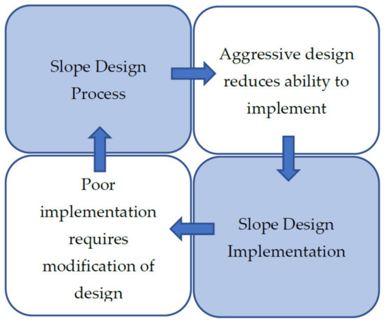
Figure 1.
A 2 × 2 interaction matrix.
A more complex example is shown in Figure 2.
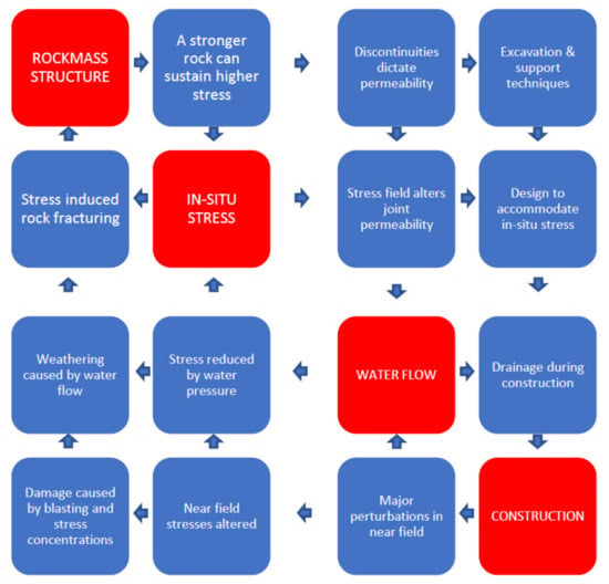
Figure 2.
An example of a simple, four-variable, binary interaction matrix (BIM), modified from [10,11]. The four main variables are rock mass structure, in situ stress, water flow, and construction, identified along the leading diagonal. The 12 binary interactions between the pairs of main variables are defined in the off-diagonal boxes.
Once constructed, this matrix is ‘coded’, ensuring the off-diagonal cells convey the importance (or support mathematical manipulation) of the matrix. Five main methods to accomplish coding are as follows:
- Binary: the mechanisms in the off-diagonal boxes are either switched on or off, so the coding is either as 1 or 0;
- Expert semi-quantitative (ESQ): a number from 0 to 4 is allocated as follows: 0—no interaction; 1—weak interaction; 2—medium interaction; 3—strong interaction; 4—critical interaction;
- According to the slope of an assumed linear relation;
- More numerically via a partial differential relation;
- Explicitly via complete numerical analysis of the mechanism.
The method recommended by Hudson [3,4] is method 2 (ESQ) because the other approaches are either too insensitive or require information that is rarely available. Once the off-diagonal terms have been coded, the values in each row can be summed to indicate a C (Cause) ordinate for a particular variable. Likewise, those in the columns can be summed to give the associated E (Effect) ordinate. The ‘intensity’ of the interaction is derived by summing C and E for each variable. Further, parameter dominance can be established by determining C–E (see Figure 3).
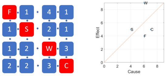
Figure 3.
The rock engineering system approach to derive parameter interaction intensity and importance for the problem shown in Figure 2. Figures modified from [11].
Thus far, only binary interactions between parameters have been considered. As discussed in [12], the fully coupled model of the process considers the interaction matrix as a mechanism network. Graph theory can be applied, and therefore, the (uncoupled) binary interaction matrix is transformed into a (fully coupled) global interaction matrix (GIM). The difference in interpretation of the two matrices and pseudocode relating the two based on [12] is shown in Figure 4.
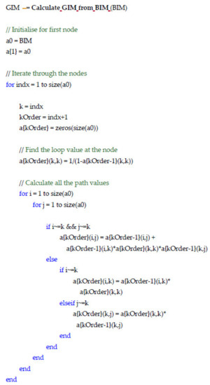
Figure 4.
(Top) Comparison of binary interact matrix (BIM) and global interaction matrix (GIM) for a two-parameter problem; (bottom) pseudocode for generation of the GIM.
After the GIM was calculated (effectively a model for the mining production), a validation process was undertaken. This involved testing using legacy data to ensure the model predictions were within acceptable tolerances with observed production.
2.2. Neural Network: Self-Organising Maps
The power of neural networks is derived from their ability to accurately scale the topology and distribution of the multi-variate input data space into a conveniently low-dimension space, which is more amenable to well-established data processing techniques. A clustering algorithm was used to sort the output of the neural network.
Self-organising maps (SOM) [13] are data-mining neural-network-based techniques for understanding relationships within a dataset. They have been used in a wide variety of geoscience and other applications including geospatial data analysis, resource characterisation, climate analysis, and human movement [14]. SOM was selected for this research since it has several benefits over other neural network approaches, including being an unsupervised process, the ability to process disparate datasets including categorical data and nulls, and the ability to support clustering of data using the principles of vector quantisation.
For this research, the SiroSOM software [15,16] was used. SiroSOM was originally trialled on mining data to investigate seismic risk [15]. It was later used for a range of other mining-related analyses including hydrothermal mineral system assessments [17], sublevel caving material recovery [18], rock strength estimation from geophysical logs [19], and lithological boundary definition [20]. Its capacity to deal with disparate and incomplete datasets, common in mining and exploration, has been proven. To the best of the authors’ knowledge, this research discloses the first attempt at using SOM for mine-production forecasting as a function of geotechnical variables.
As described in [13], the self-organising map is an artificial neural network that is based on an unsupervised learning model which maintains the topology between input and output spaces. The nodes of the network arrange themselves during the training process, hence the term ‘self-organising’. This important property makes it suitable for reducing multi-dimensional problems into the more readily interpreted two-dimensional space whilst conserving the salient structural aspects of the data.
Unlike typical neural networks, the structure comprises a single 2D grid of neurons. Nodes are directly connected to input data but not each other. The weights of these connections are updated using a competitive learning process during which all nodes compete for the right to respond to the input data vector. At the end of the process, the so-called best-matching units, or most similar nodes, are distributed topologically in accordance with the data with similar nodes located relatively close to each other.
The SOM algorithm can be described mathematically as shown in Figure 5. In this syntax, w_ij represents a vector of weights of the connections between node(i,j) and its neighbours.
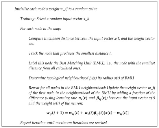
Figure 5.
SOM algorithm.
2.3. Proposed Algorithm
By using RES and SOM, an algorithm can be constructed which satisfies the requirements of the method—namely,
- Support construction of a model capturing complex multi-variable interactions between geotechnical conditions and mining production;
- Prediction of future production based on this model.
Figure 6 shows the proposed algorithm. The two processing streams occur in parallel, with BIM construction, coding, analysis, and simplification (updating), informing the historical data acquisition process, GIM construction, and validation. The forecasts produced at the end of both the modelling and neural network processes are then compared and checked for consistency.
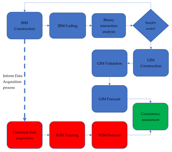
Figure 6.
Proposed algorithm.
2.4. Implementation of Algorithm
In this research, several tools were used to implement the algorithm shown in Figure 6.
Construction and coding of BIM
A spreadsheet (MS Excel) was used to capture the parameters, construct the BIM and perform the scoring.
Construction and validation of GIM
The software was implemented in MATLAB [21] to implement the GIM algorithm, as described in Figure 4. A series of unit test scenarios were implemented to validate the derived GIM.
Construction of the SOM
The CSIRO software SiroSOM [22] was used to conduct the SOM analysis.
Consistency assessment
The software was implemented in MATLAB to compare the SOM model predictions and report appropriate statistics.
3. Results: Semi-Synthetic Analysis
3.1. Production Data Provided by the Site
An operating coal mine in southern Queensland, referred to as Site A, served as the study site for this research. Initially, the site expected to be able to access previously recorded historical data including information about quantities and rates of overburden, interburden, and waste moved as the strips were mined. Further, the dataset was also to include information on structurally related rock mass incidents (such as instabilities, failures) that affected material handling, hazard reduction activities, and ultimately, production. Such data would be used for analysis to examine correlations between geological conditions to operational efficiency, thereby demonstrating the value of superior predictions of conditions ahead of mining.
Difficulties were encountered in accessing legacy databases or extracting useful, reliable, and high (spatial and temporal) resolution data. As a result, only coarse, high-level data for the aforementioned variables could be made available.
The confidential production dataset provided by Site A consists of aggregated bulk material movements for several highwall strips at the site that had been previously accessed study sites for the authors. In this current form, the data were deemed to have an insufficient temporal resolution to fully test the forecasting capabilities of the algorithm being developed in this research, since the following additional detail was required:
- Data corresponding to bulk movements as a function of time and/or mining progress per strip;
- Operational data (highwall inspection reports, blast engineer reports, dozer operation reports) and other data that detail operational delays, once again as a function of time and/or mining progress per strip.
After discussions with site personnel, it was decided to use a semi-synthetic data approach, based on an analysis of the coarse, high-resolution production data provided by the site, an understanding of the site conditions as described by the site engineers, and based on the authors’ previous geotechnical investigations at the site. The parameters used in the analysis were constrained to those used at the site (and other coal mining operations) and were readily available to the mining engineer during the mining process.
The sources of data likely to be available to the mining engineer of any given mining operation, as described in [2], include the following data:
- Rock mass characterisation (geological model, hydrogeological model, structural mapping, potentially geophysics and slope design modelling, and analyses);
- Site characterisation and production data (design parameters, drill and blast reports, production data (including deviations from planned), and hazard reports).
To establish the important parameters that are required for consideration, and to facilitate the development of a production model, the rock engineering system (RES) analytical approach was used.
3.2. Semi-Synthetic Production Data Analysis
Typical parameter values were estimated from the actual site data. Assumptions on the frequency of sampling (i.e., daily) were made for relevant parameters.
3.2.1. RES for System Decomposition
A RES expert elicitation session was undertaken to decompose the problem as outlined in the RES method. This would normally be undertaken by mining engineering personnel. From the RES elicitation session, important parameters were identified that would be used for developing the causal model (Table 1).

Table 1.
Parameters used in initial RES matrix (R = rock, S = site, P = project engineering, O = output).
As discussed in Section 2.1, the RES approach requires expert judgement and experience to be used to derive an ‘interaction matrix’ determining the degree to which different parameters or variables interact (Table 1, Table 2 and Table 3).

Table 2.
Set codes and colour coding.

Table 3.
Scoring values and definitions.
Considering that the matrix in Figure 7 was generated for demonstration purposes, and that, in practice, the site’s geotechnical and production teams would generate this through a debate/discussion process to meet consensus, the following observations can be made:
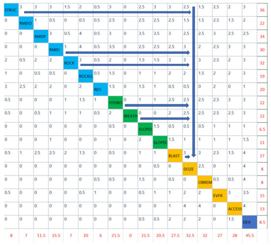
Figure 7.
BIM matrix after scoring. For example, that structure, RMDI, rock type, hydrogeology, weather, and blast have strong interactions with dozer operation’s success.
- Weather, blast, dozer, overburden removal, and access have critical interactions with deviation from planned;
- Structure, RMPD, and rock type have strong interactions with the blast success;
- Structure, RMDI, rock type, hydro, weather, and blast have strong interactions with dozer operations’ success.
As previously described in Section 2.1, summing the columns and rows of the BIM yields the cause–effect metrics. These metrics can provide an initial assessment of how active a particular variable is within the matrix system (interaction ‘intensity’, cause + effect) and variable dominance (cause–effect).
When sorted based on intensity, the variables are (in ascending order) as follows:
WEATH, REG, SLOPEOL, RMDO, SLOPEDIM, ROCK, ROCKQ, OBREM, DOZE, ACCESS, EVFR, HYDRO, STRUC, RMDP, RMDI, BLAST.
When sorted based on dominance, they are (in ascending order) as follows:
DOZE, OBREM, SLOPEOL, ACCESS, EVFR, SLOPEDIM, ROCKQ, BLAST, HYDRO, REG, RMDO, RMDI, WEATH, RMDP, ROCK, STRUC.
The variables shown in bold have negative dominance (the system’s effect on the variable is greater than the variable’s effect on the system).
The cause–effect data are also plotted in Figure 8 which assists this interpretation. From this analysis, we can deduce the following characteristics of the system:
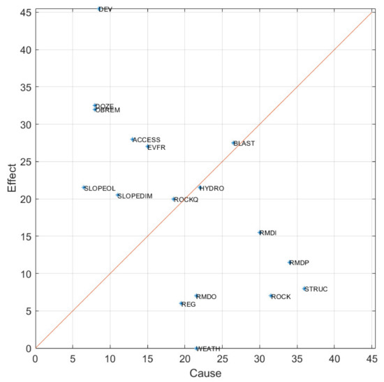
Figure 8.
Cause-effect plot based on the BIM presented in Figure 7.
The three most dominant parameters (Cause > Effect) are STRUC, ROCK, and RMDP. The three most subordinate parameters (Effect > Cause) are DOZE, OBREM, and SLOPEOL. This is consistent with the somewhat intuitive interpretation that the rock conditions dominate, and the system most greatly impacts dozer operations, overburden removal rates, and, consequently, slope design.
After this initial assessment, simplification of the BIM was deemed to be possible and after analysis of parameter hierarchy, the parameter list was reduced to 10, as shown in Table 4. This was justified as follows:

Table 4.
Reduced parameter list used in initial RES matrix (R = rock, S = site, P = project engineering, O = output).
- The rock quality parameter is a function of rock type and structure properties such as fracture intensity (itself a function of structure orientation and persistence);
- Deviation from the plan is a function of other production variables such as overburden removal, dozer effectiveness, and ramp access.
3.2.2. RES for Model Simulation
Under normal circumstances, the RES matrix would be used by the mine site to predict the deviation of production from the plan (DEV). In this research, due to the lack of actual high resolution production-related data, the RES interaction matrix was also used to assist simulation. Data synthesis was undertaken as follows:
- The binary interaction matrix (BIM) was used to establish a reasonable causal model, and a global interaction matrix (GIM) was computed (Section 2.1);
- Input parameters were modelled as random variables;
- Perturbations (e.g., rainfall event) were modelled as Gaussian ‘wavelets’;
- A total of 100 samples across a highwall were modelled, assuming each sample corresponds to 1 day of operations.
A mining production scenario was created to serve as the basis of the analysis. For the first 100 days of mining, the following conditions were simulated:
- Structural complexity increased gradually peaking around day 50;
- Weather conditions were favourable for most of the time but degraded, peaking on day 80;
- Geotechnical hazard events peaked on day 50.
The 100 days of data were used to train the algorithm described in Section 2.2. A subsequent set of data for the following 100 days were also simulated, for the following scenario:
- Structural complexity peaks on two occasions, days 15 and 75;
- Weather is good throughout but degrades for final 30 days;
- As with structural complexity, event frequency also peaks twice, increasing from days 20 to 40 and 90 to 100.
Figure 9 and Figure 10 show realisations of the simulated deviation from planned (DEV) and the input parameters for the first and second 100 days, respectively. Both input (uncoupled) and output (fully coupled) traces are shown.
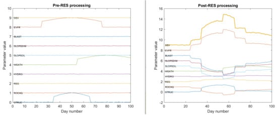
Figure 9.
Simulated production data for the first 100 days (bold orange trace on right) and input RES parameters (non-bold traces) as a function of highwall strike distance. Traces have vertical offsets for clarity. The left figure shows inputs (uncoupled), and the right shows fully coupled outputs from the model.
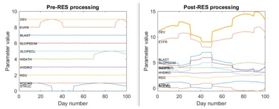
Figure 10.
Simulated production data for the second 100 days (bold orange trace on right) and input RES parameters (non-bold traces) as a function of highwall strike distance. Traces have vertical offsets for clarity. The left figure shows inputs (uncoupled), and the right shows fully coupled outputs from the model.
SiroSOM was used to apply the SOM to these data. The software parameters used are shown in Table 5.

Table 5.
SOM parameters used in the data processing.
The method selects the number of clusters that it identifies within the dataset but also allows the user to define the number if required.
Five clusters were selected in this case (Figure 11 and Figure 12) as a reasonable division of the 100 samples (days). Four or fewer clusters were found to make each too ‘general’, and more than five caused some of the clusters to host too few samples to be of value. With a much larger dataset, it would be possible to assess whether there are more than five naturally occurring clusters.
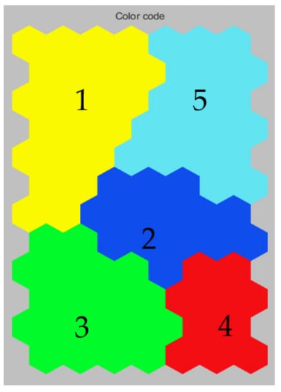
Figure 11.
SOM clusters: the data clusters are based on each sample’s characteristics, comparing each with all other samples and seeking relationships between them.

Figure 12.
Centroid values. The SOM program provides a ‘centroid value’ for each cluster or set of data. Each sample is then assigned a cluster, whose centroid is most similar to its own values.
For the purpose of this project, the SOM network was trained on the first 100 days of simulated data that was presented in Section 3.2. All 100 samples and all 10 variables were used in the training dataset, to generate the SOM map that would act as the supervisory tool. Several iterations were performed to identify a suitable number of clusters with unique sets of attributes. Each cluster has a ‘centroid value’ (Figure 12) with which every sample was compared and assigned to the closest matching centroid.
Based on the closest centroid values, SOM assigned each sample to a given cluster as follows:
- Cluster 1 n = 34;
- Cluster 2 n = 10;
- Cluster 3 n = 20;
- Cluster 4 n = 11;
- Cluster 5 n = 25.
Component plots were compared, and it was ascertained that associations between them reflected the relationships considered in the RES matrix. Components were also shown to correlate negatively or positively with changes in the conditions, as shown in Figure 13.
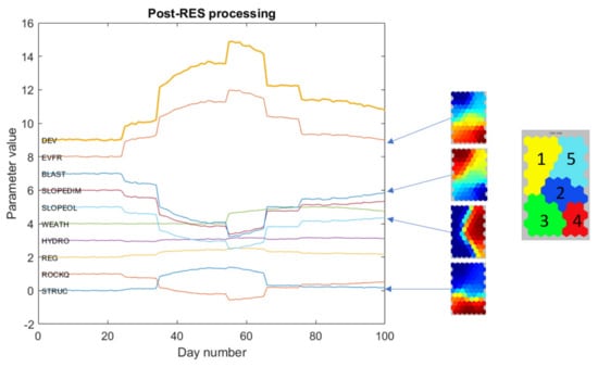
Figure 13.
Results of the SOM training show the relationships with selected SOM components.
The DEV data were reduced to Nulls and presented into SiroSOM against the supervisory SOM. Supplied only with 9 parameters, the non-DEV parameter data were predicted as missing values, based on associations within the previous 100 days and those in the remaining 9 parameters. The results (predicted DEV) compared with previously calculated DEV, are shown in Figure 14. Figure 14b also shows the difference between the SOM and RES results. The root-mean-square error (RMSE) is approximately 0.4. It demonstrates very good predictive capabilities. As with all neural networks, this performance assumes that the training data capture the salient parameter interactions. In practice, this means the larger the dataset is, the better are the results. This is consistent with the approach adopted in this research—namely, the acquisition of data from more mining strips will improve the prediction of conditions in future strips.
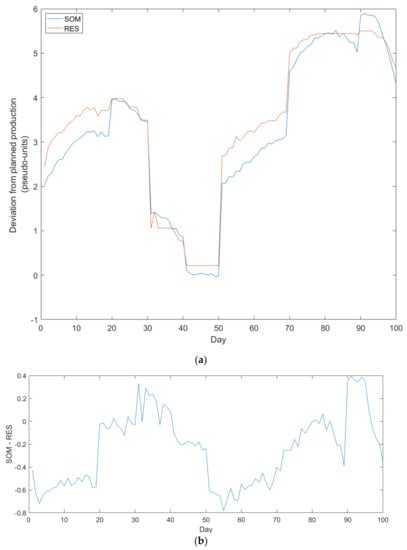
Figure 14.
Results of the SOM prediction; good agreement between SOM prediction (blue) and RES model (red) is shown in (a), and the difference is shown in (b).
4. Discussion and Conclusions
The feasibility of predicting mining production as a function of critical geotechnical and other parameters was demonstrated. It relies on a conceptual causal model of parameter dependencies to be developed, formulated into a computational model (we recommend the use of RES for this purpose) and used to define the input vector of historical data for training a neural network (we used SOM in this research). The trained network can then be used to predict the response of production to changes in these parameters as they are quantified during mining.
Although the proposed method shows great promise for operating mining sites, this research highlighted several implementation considerations.
The difficulties in accessing legacy databases at Site A is an issue common to most mining operations. For the proposed method to deliver the most value to mining operations, ready access to operational data acquired over previous mining phases is required. This likely necessitates the maintenance of a centralised database to support the progressive accumulation of spatiotemporal data required to characterise parameters outlined in Table 4, including operational data (highwall inspection reports, blast engineer reports, dozer operation reports, and other data that detail operational delays such as overburden removal rates, wall scaling, clean-up, etc.). This suggests that mining operations will require well-defined processes for the acquisition, archiving, and retrieval of these data during mining operations.
Author Contributions
Conceptualization, M.E., J.H. & P.D.; methodology, M.E., J.H. & P.D.; software, M.E., J.H. & P.D.; validation, M.E., J.H. & P.D.; formal analysis, M.E., J.H. & P.D.; investigation, M.E., J.H. & P.D.; resources, M.E., J.H. & P.D.; data curation, M.E., J.H. & P.D..; writing—original draft preparation, M.E.; writing—review and editing, M.E., J.H. & P.D.; visualization, M.E., J.H. & P.D.; supervision, M.E.; project administration, M.E.; funding acquisition, M.E. All authors have read and agreed to the published version of the manuscript.
Funding
This study was financially supported by the Australian Coal Association Research Program (ACARP) through Project C27011.
Acknowledgments
This work formed part of Project C27011, which was undertaken in collaboration with University of Newcastle researchers and we are grateful to Anna Giacomini, Olivier Buzzi, and Stephen Fityus. We appreciate the support from the industry monitors Gift Makusha, Walter Keilich, Leonie Bradfield, and Warren Hitchcock for their helpful comments and suggestions, and Anglo, BHP, Thiess, Stanwell, and Downer EDI, particularly Dave Edwards, for providing data. Finally, we are grateful to Binzhong Zhou for his review and improvements to the manuscript.
Conflicts of Interest
The authors declare no conflict of interest. The funders had no role in the design of the study; in the collection, analyses, or interpretation of data; in the writing of the manuscript, or in the decision to publish the results.
References
- Jele, R.; Dunn, M. Economic significance of geotechnical uncertainties in open pit mines. In Mining Geomechanical Risk; Australian Centre for Geomechanics: Perth, Australia, 2019. [Google Scholar]
- Read, J.; Stacey, P. Guidelines for Open Pit Design; CSIRO Publishing: Clayton, Australia, 2009. [Google Scholar]
- Arrieta, A.B.; Díaz-Rodríguez, N.; Del Ser, J.; Bennetot, A.; Tabik, S.; Barbado, A.; García, S.; Gil-López, S.; Molina, D.; Benjamins, R.; et al. Explainable Artificial Intelligence (XAI): Concepts, taxonomies, opportunities and challenges toward responsible AI. Inf. Fusion 2020, 58, 82–115. [Google Scholar] [CrossRef] [Green Version]
- Chattopadhyay, A.; Manupriya, P.; Sarkar, A.; Balasubramanian, V.N. Neural Network Attributions: A Causal Perspective. In Proceedings of the 36th International Conference on Machine Learning (ICML2019), Long Beach, CA, USA, 9–15 June 2019. [Google Scholar]
- MathWorks. SimulLink. MathWorks. Available online: https://au.mathworks.com/products/simulink.html (accessed on 31 October 2021).
- ORE. Integrated Extraction Simulator. CRC ORE. Available online: https://www.crcore.org.au/ies (accessed on 31 October 2021).
- GoldSim. Available online: https://www.goldsim.com/ (accessed on 31 October 2021).
- Abiodun, O.I.; Jantan, A.; Omolara, A.E.; Dada, K.V.; Mohamed, N.A.; Arshad, H. State-of-the-art in artificial neural network applications: A survey. Heliyon 2018, 4, e00938. [Google Scholar] [CrossRef] [PubMed] [Green Version]
- Karimi, D.; Dou, H.; Warfield, S.K.; Gholipour, A. Deep learning with noisy labels: Exploring techniques and remedies in medical image analysis. Med. Image Anal. 2020, 65, 101759. [Google Scholar] [CrossRef] [PubMed]
- Hudson, J. Rock Engineering Systems: Theory and Practice; Ellis Horwood Ltd.: Chichester, UK, 1992. [Google Scholar]
- Hudson, J. A review of Rock Engineering Systems applications over the last 20 years. In Rock Characterisation, Modelling and Engineering Design Methods; Taylor & Francis Group: London, UK, 2013; pp. 419–424. [Google Scholar]
- Jiao, Y.; Hudson, J. The Fully-Coupled Model for Rock Engineering Systems. Int. J. Rock. Mech. Min. Sci. Geomech. 1995, 32, 491–512. [Google Scholar] [CrossRef]
- Kohonen, T. Self-Organizing Maps: Third Extended Edition; Springer Series in Information Sciences: Berlin, Germany, 2001; Volume 30. [Google Scholar]
- Agarwal, P.; Skupin, A. Self-Organising Maps: Applications in Geographic Information Science; Agarwal, P., Skupin, A., Eds.; John Wiley & Sones Ltd.: Chichester, UK, 2008; p. 214. [Google Scholar]
- Fraser, S. Proposal for Pilot Study into the Effectiveness of “CSOM” as a Predictive Tool for Forecasting Seismicity at the Mine Design Stage at Mt Charlotte, Kalgoorlie, Western Australia; CSIRO Exploration and Mining: Clayton, Australia, 2004. [Google Scholar]
- Fraser, S.; Mikula, P.; Lee, M.; Dickson, B.; Kinnersly, E. Data Mining Mining Data: Ordered Vector Quantization and its Application to Mine Geotechnical Data Sets. In Proceedings of the 6th International Mining Geology Conference, Rising to the Challenge, Darwin, Australia, 21–23 August 2006. [Google Scholar]
- Lersisi, J.; Sonjonen-Ward, P.; Fraser, S.; Ruotsalainen, A. Assessment of hydrothermal processes associated with Proterozoic mineral systems in Finland using self-organizing maps. In Proceedings of the EGU General Assembly Conference Abstracts, Vienna, Austria, 19–24 April 2009. [Google Scholar]
- Brunton, I.D.; Fraser, S.J.; Hodgkinson, J.H.; Stewart, P.C. Parameters influencing full scale sublevel caving material recovery at the Ridgeway gold mine. Int. J. Rock Mech. Min. Sci. 2009, 47, 647–656. [Google Scholar] [CrossRef]
- Zhou, B.; Fraser, S.; Borsaru, M.; Aizawa, T.; Sliwa, R.; Hashimoto, T. New Approaches for Rock Strength Estimation from Geophysical Logs. In Proceedings of the Bowen Basin Symposium, Yeppoon, QLD, Australia, 12–14 October 2005. [Google Scholar]
- Hodgkinson, J.H.; Fraser, S.J.; Donchak, P. Using self-organising maps to derive lithological boundaries from geophysically-derived data in the Mt. Isa region, Queensland. In Proceedings of the 22nd ASEG Conference, Brisbane, Australia, 26–29 February 2012. [Google Scholar]
- Mathworks, MATLAB Mathworks. Available online: https://au.mathworks.com/products/matlab.html (accessed on 31 October 2021).
- CSIRO. SiroSOM, CSIRO. Available online: https://www.csiro.au/en/work-with-us/industries/mining-resources/exploration/self-organising-maps (accessed on 31 October 2021).
Publisher’s Note: MDPI stays neutral with regard to jurisdictional claims in published maps and institutional affiliations. |
© 2021 by the authors. Licensee MDPI, Basel, Switzerland. This article is an open access article distributed under the terms and conditions of the Creative Commons Attribution (CC BY) license (https://creativecommons.org/licenses/by/4.0/).