
One-Dimensional Convolutional Neural Network for Drill Bit Failure Detection in Rotary Percussion Drilling

 , ,
, ,
Abstract
:1. Introduction
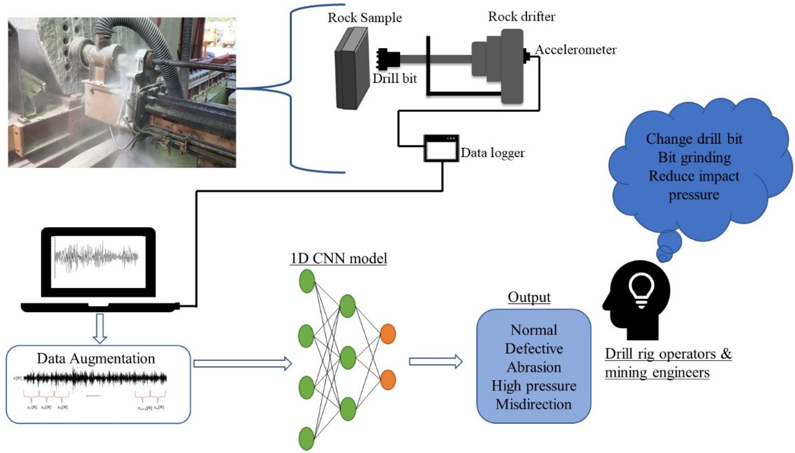
- A reliable, automatic, and cost-effective method to monitor drill bit failures using machine learning. The use of accelerometers allows for easy installation and removal. Accelerometers can be used with any drilling machine, thereby making the system easy to adopt and implement. 1D CNN has the advantage of processing and analyzing complex tasks in a short time, which allows the automation of decision making, therefore eliminating the unreliable method used by drill rig operators.
- Compared to other fault diagnosis studies which are based on heavy data pre-processing and are limited to two classifications, normal and failure, this paper presents a system that requires minimal data pre-processing, making it easy to implement in real-time. The system also classifies five conditions: normal, defective, abrasion, high impact pressure, and misdirection.
- The application of a longer kernel size that is approximately ¼ the size of the input signal effectively improves the accuracy of the drill bit failure detection model.
2. 1D CNN for Time Series Classification
3. Materials and Methods
3.1. Data Description
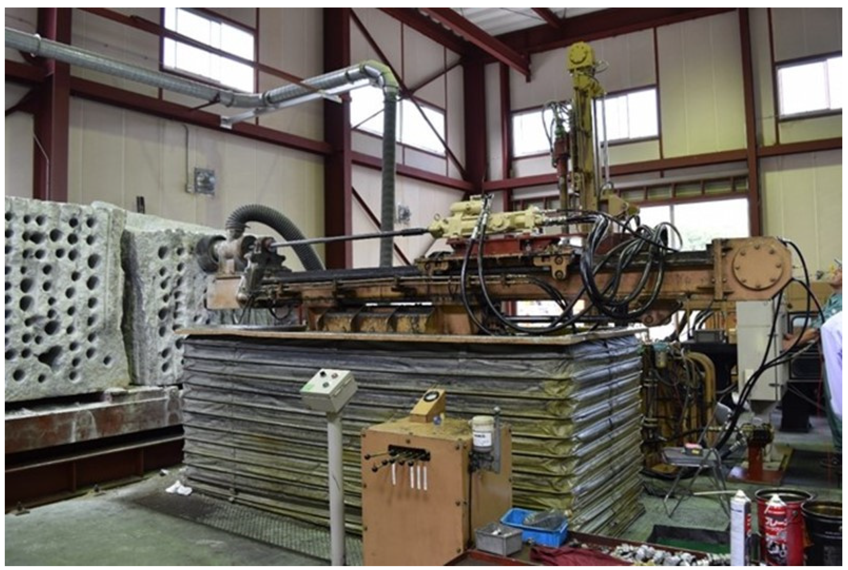
3.2. Data Acquisition
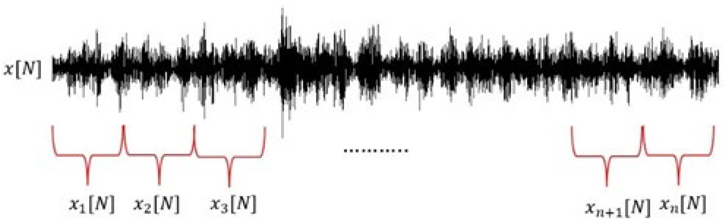
3.3. Data Preprocessing
3.4. State of the Art Deep Learning Neural Networks
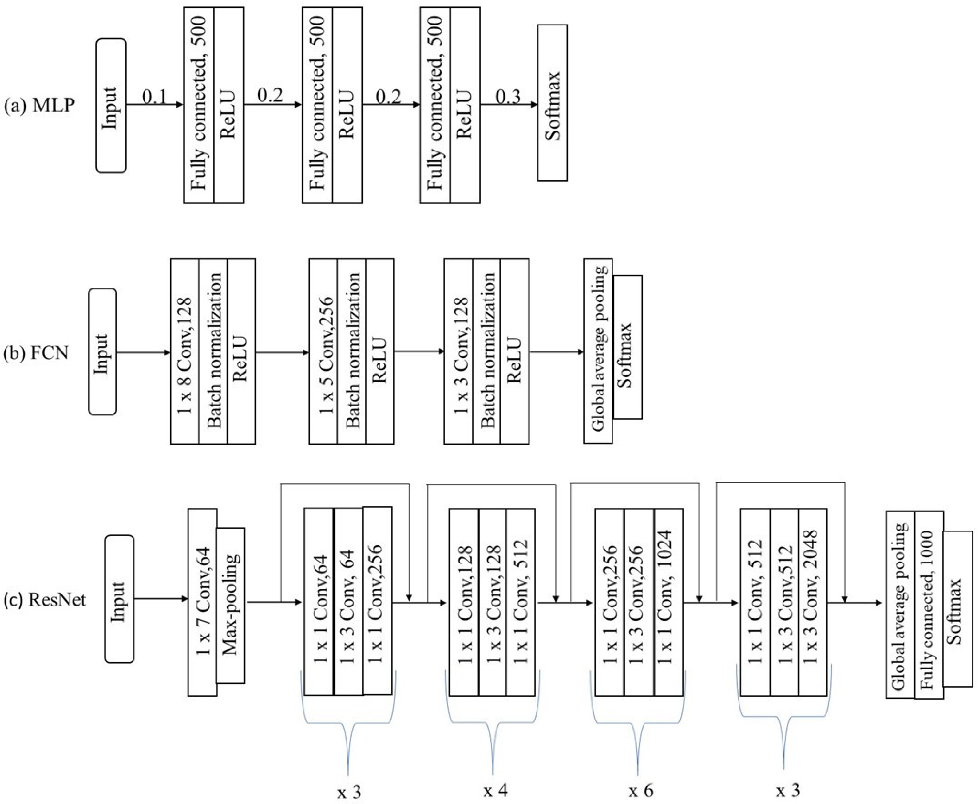
3.4.1. Multilayer Perceptron (MLP)
3.4.2. Fully Connected Layers (FCN)
3.4.3. Residual Network (ResNet 50)
3.5. Experiment Implementation Details
3.6. Evaluation Metrics
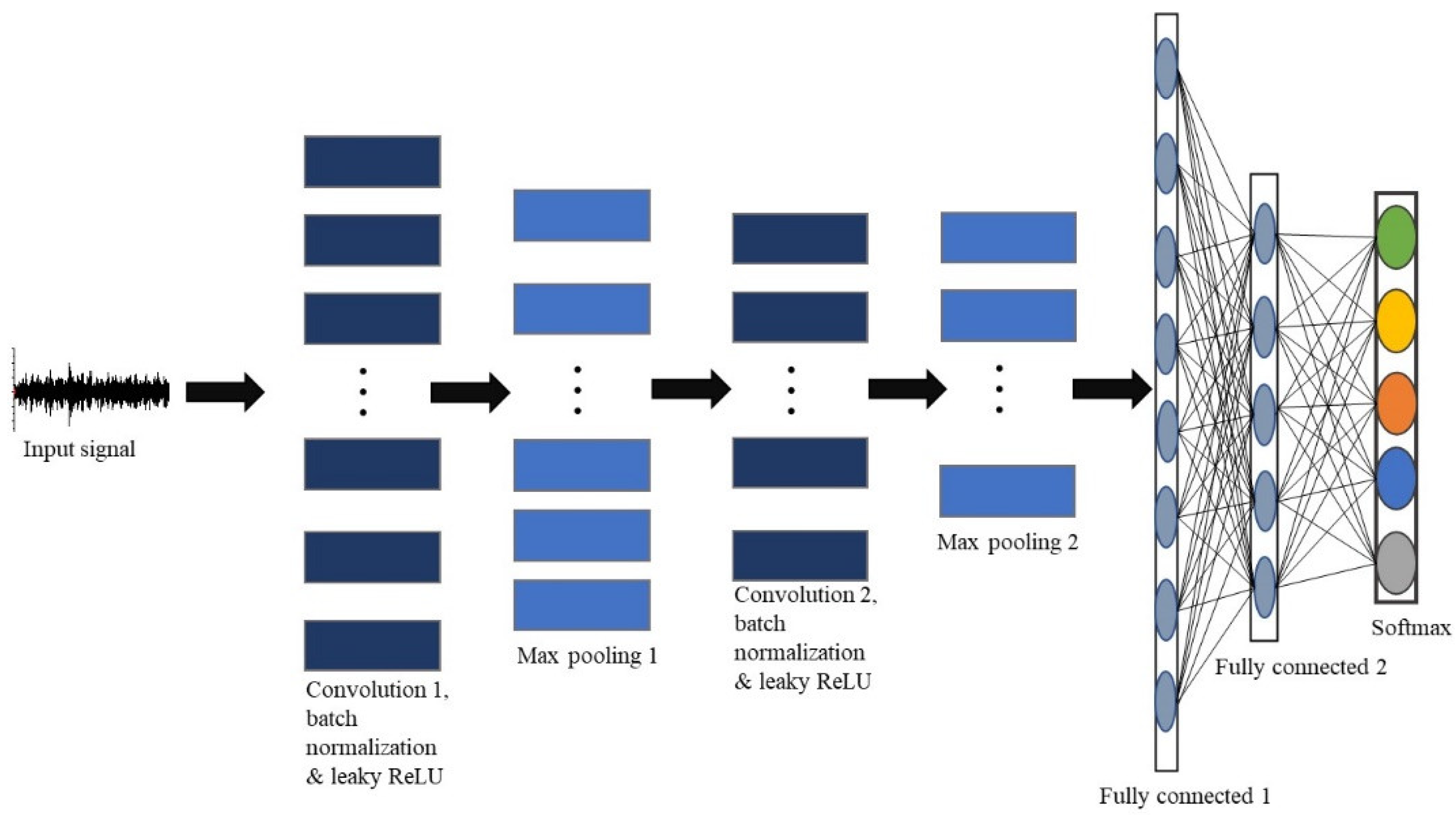
4. Proposed Drill Bit Failure Detection (DBFD) Model 1D CNN Architecture
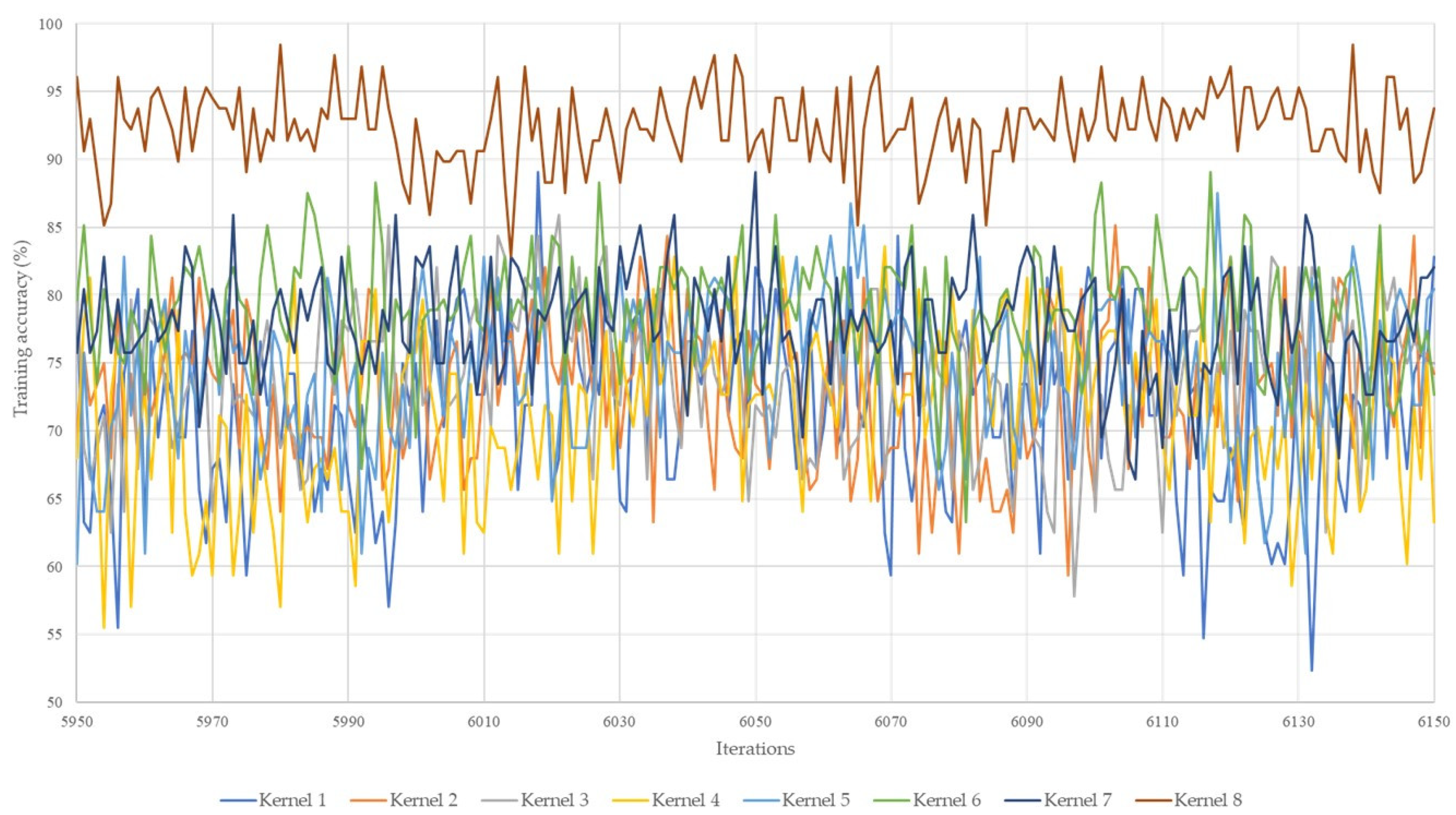
4.1. Kernel Size
4.2. Pooling Method and Size
4.3. Number of Convolution Filters
4.4. Evaluation of Network Depth on the Performance of the DBFD Model
5. Results and Discussions
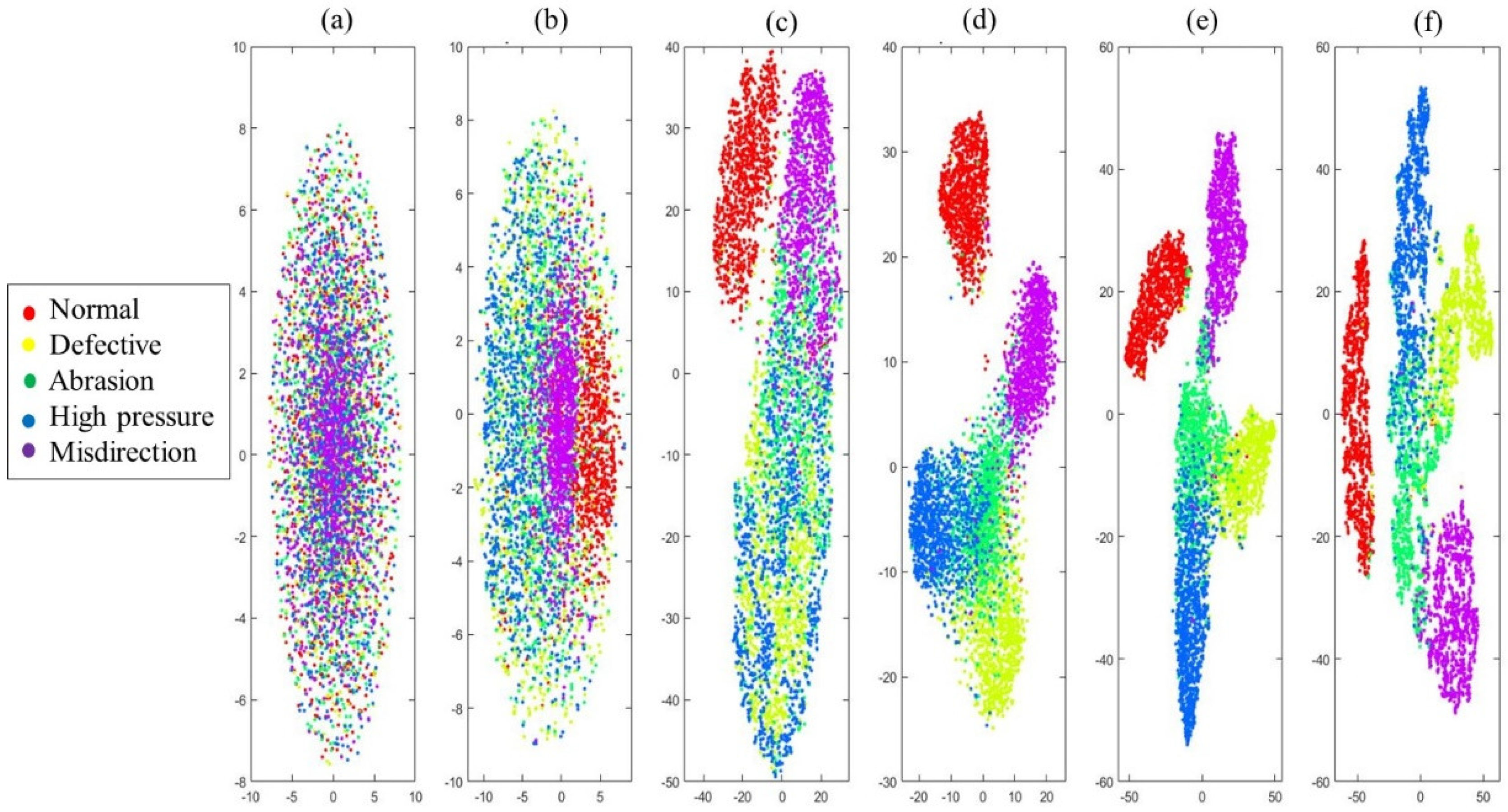
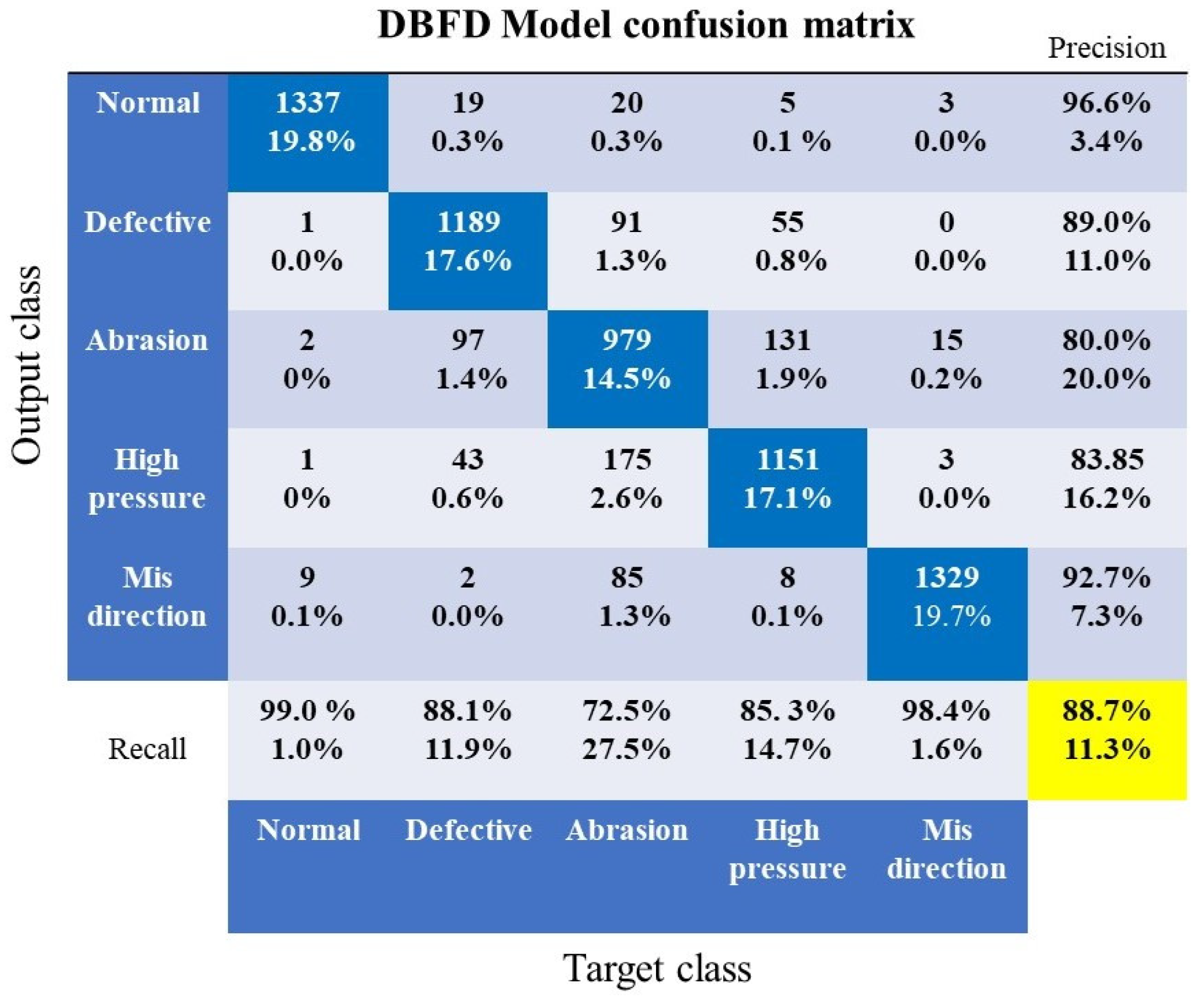
5.1. DBFD Model Evaluation
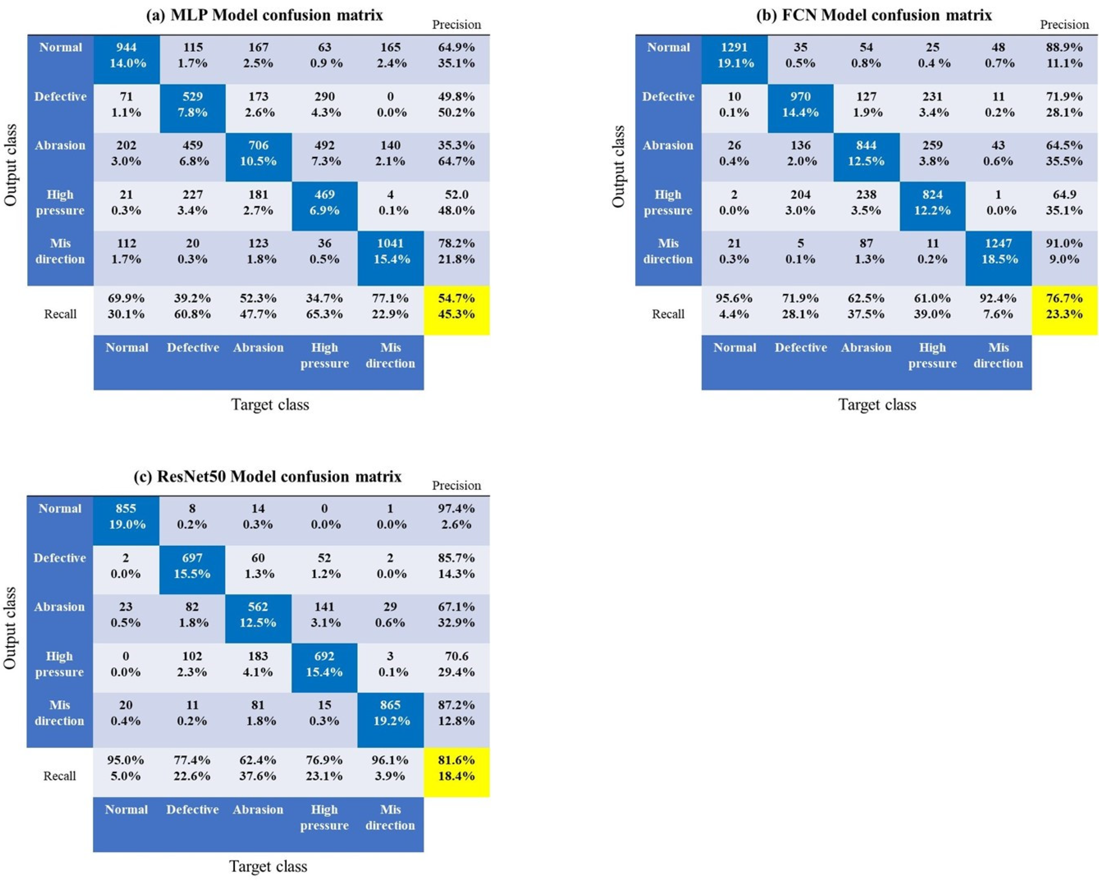
5.2. Comparison with SOTA Models
6. Conclusions
Author Contributions
Funding
Acknowledgments
Conflicts of Interest
References
- Sandvik Tamrock Corp. Rock Excavation Handbook; Sandvik Tamrock Corp: Stockholm, Sweden, 1999. [Google Scholar]
- Jang, H. Effects of Overused Top-hammer Drilling Bits. IMST 2019, 1, 555558. [Google Scholar] [CrossRef]
- Gradl, C.; Eustes, A.W.; Thonhauser, G. An Analysis of Noise Characteristics of Drill Bits; ASME: Estoril, Portugal, 2008; p. 7. [Google Scholar]
- Karakus, M.; Perez, S. Acoustic emission analysis for rock–bit interactions in impregnated diamond core drilling. Int. J. Rock Mech. Min. Sci. 2014, 68, 36–43. [Google Scholar] [CrossRef]
- Kawamura, Y.; Jang, H.; Hettiarachchi, D.; Takarada, Y.; Okawa, H.; Shibuya, T. A Case Study of Assessing Button Bits Failure through Wavelet Transform Using Rock Drilling Induced Noise Signals. J. Powder Metall. Min. 2017, 6, 1–6. [Google Scholar] [CrossRef]
- Sikorska, J.Z.; Mba, D. Challenges and obstacles in the application of acoustic emission to process machinery. Proc. Inst. Mech. Eng. Part E J. Process. Mech. Eng. 2008, 222, 1–19. [Google Scholar] [CrossRef]
- Jantunen, E. A summary of methods applied to tool condition monitoring in drilling. Int. J. Mach. Tools Manuf. 2002, 42, 997–1010. [Google Scholar] [CrossRef]
- Uğurlu, Ö.F. Drill Bit Monitoring and Replacement Optimization in Open-Pit Mines. Bilimsel Madencilik Derg. 2021, 60, 83–87. [Google Scholar] [CrossRef]
- Jung, D.; Choi, Y. Systematic Review of Machine Learning Applications in Mining: Exploration, Exploitation, and Reclamation. Minerals 2021, 11, 148. [Google Scholar] [CrossRef]
- Vununu, C.; Moon, K.-S.; Lee, S.-H.; Kwon, K.-R. A Deep Feature Learning Method for Drill Bits Monitoring Using the Spectral Analysis of the Acoustic Signals. Sensors 2018, 18, 2634. [Google Scholar] [CrossRef] [PubMed] [Green Version]
- Rai, B. A Study of Classification Models to Predict Drill-Bit Breakage Using Degradation Signals. Int. J. Econ. Manag. Eng. 2014, 8, 4. [Google Scholar]
- Gómez, M.P.; Hey, A.M.; Ruzzante, J.E.; D’Attellis, C.E. Tool wear evaluation in drilling by acoustic emission. Phys. Procedia 2010, 3, 819–825. [Google Scholar] [CrossRef] [Green Version]
- Bello, O.; Teodoriu, C.; Yaqoob, T.; Oppelt, J.; Holzmann, J.; Obiwanne, A. Application of Artificial Intelligence Techniques in Drilling System Design and Operations: A State of the Art Review and Future Research Pathways. In Proceedings of the SPE Nigeria Annual International Conference and Exhibition, Lagos, Nigeria, 2–4 August 2016. [Google Scholar] [CrossRef]
- Lashari, S.E.Z.; Takbiri-Borujeni, A.; Fathi, E.; Sun, T.; Rahmani, R.; Khazaeli, M. Drilling performance monitoring and optimization: A data-driven approach. J. Petrol. Explor. Prod. Technol. 2019, 9, 2747–2756. [Google Scholar] [CrossRef] [Green Version]
- Kiranyaz, S.; Avci, O.; Abdeljaber, O.; Ince, T.; Gabbouj, M.; Inman, D.J. 1D convolutional neural networks and applications: A survey. Mech. Syst. Signal Process. 2021, 151, 107398. [Google Scholar] [CrossRef]
- Eren, L. Bearing Fault Detection by One-Dimensional Convolutional Neural Networks. Math. Probl. Eng. 2017, 2017, 8617315. [Google Scholar] [CrossRef] [Green Version]
- Ince, T.; Kiranyaz, S.; Eren, L.; Askar, M.; Gabbouj, M. Real-Time Motor Fault Detection by 1-D Convolutional Neural Networks. IEEE Trans. Ind. Electron. 2016, 63, 7067–7075. [Google Scholar] [CrossRef]
- Sadouk, L. CNN Approaches for Time Series Classification. In Time Series Analysis—Data, Methods, and Applications; Ngan, C.-K., Ed.; IntechOpen: London, UK, 2019. [Google Scholar] [CrossRef] [Green Version]
- Fawaz, H.I.; Forestier, G.; Weber, J.; Idoumghar, L.; Muller, P.-A. Deep learning for time series classification: A review. Data Min. Knowl. Dis. 2019, 33, 917–963. [Google Scholar] [CrossRef] [Green Version]
- Guttenkunst, E. Study of the Wear Mechanisms for Drill Bits Used in Core Drilling; Uppsala Universitet: Uppsala, Sweden, 2018. [Google Scholar]
- Wang, Z.; Yan, W.; Oates, T. Time Series Classification from Scratch with Deep Neural Networks: A Strong Baseline. arXiv 2016, arXiv:1611.06455. [Google Scholar]
- He, K.; Zhang, X.; Ren, S.; Sun, J. Deep Residual Learning for Image Recognition. In Proceedings of the 2016 IEEE Conference on Computer Vision and Pattern Recognition (CVPR), Las Vegas, NV, USA, 27–30 June 2016; pp. 770–778. [Google Scholar] [CrossRef] [Green Version]
- Guennec, A.L.; Malinowski, S.; Tavenard, R. Data Augmentation for Time Series Classification Using Convolutional Neural Networks; Halshs-01357973; ECML/PKDD Workshop on Advanced Analytics and Learning on Temporal Data: Riva Del Garda, Italy, 2016. [Google Scholar]
- Zhao, B.; Lu, H.; Chen, S.; Liu, J.; Wu, D. Convolutional neural networks for time series classification. J. Syst. Eng. Electron. JSEE 2017, 28, 162–169. [Google Scholar] [CrossRef]
- Tang, W.; Long, G.; Liu, L.; Zhou, T.; Jiang, J.; Blumenstein, M. Rethinking 1D-CNN for Time Series Classification: A Stronger Baseline. arXiv 2021, arXiv:2002.10061. [Google Scholar]
- Peng, D.; Liu, Z.; Wang, H.; Qin, Y.; Jia, L. A Novel Deeper One-Dimensional CNN with Residual Learning for Fault Diagnosis of Wheelset Bearings in High-Speed Trains. IEEE Access 2019, 7, 10278–10293. [Google Scholar] [CrossRef]
- Ghosh, A.; Sufian, A.; Sultana, F.; Chakrabarti, A.; De, D. Fundamental Concepts of Convolutional Neural Network. In Recent Trends and Advances in Artificial Intelligence and Internet of Things; Balas, V.E., Kumar, R., Srivastava, R., Eds.; Springer International Publishing: Cham, Switzerland, 2020; Volume 172, pp. 519–567. [Google Scholar] [CrossRef]
- Ahmed, W.S.; Karim, A.A.A. The Impact of Filter Size and Number of Filters on Classification Accuracy in CNN. In Proceedings of the 2020 International Conference on Computer Science and Software Engineering (CSASE), Duhok, Iraq, 16–18 April 2020; pp. 88–93. [Google Scholar] [CrossRef]
- Khan, A.; Sohail, A.; Zahoora, U.; Qureshi, A.S. A Survey of the Recent Architectures of Deep Convolutional Neural Networks. Artif. Intell. Rev. 2020, 53, 5455–5516. [Google Scholar] [CrossRef] [Green Version]
- Maaten, L.V.D.; Geoffrey, H. Visualizing Data Using t-SNE. Mach. Learn. Res. 2008, 9, 2579–2605. [Google Scholar]


| Conditions | Type of Bit | Number of Holes | Number of Hits per Minute | Length (m) | Time (s) |
|---|---|---|---|---|---|
| Normal | Normal | 10 | 3120 | 1 | 60 |
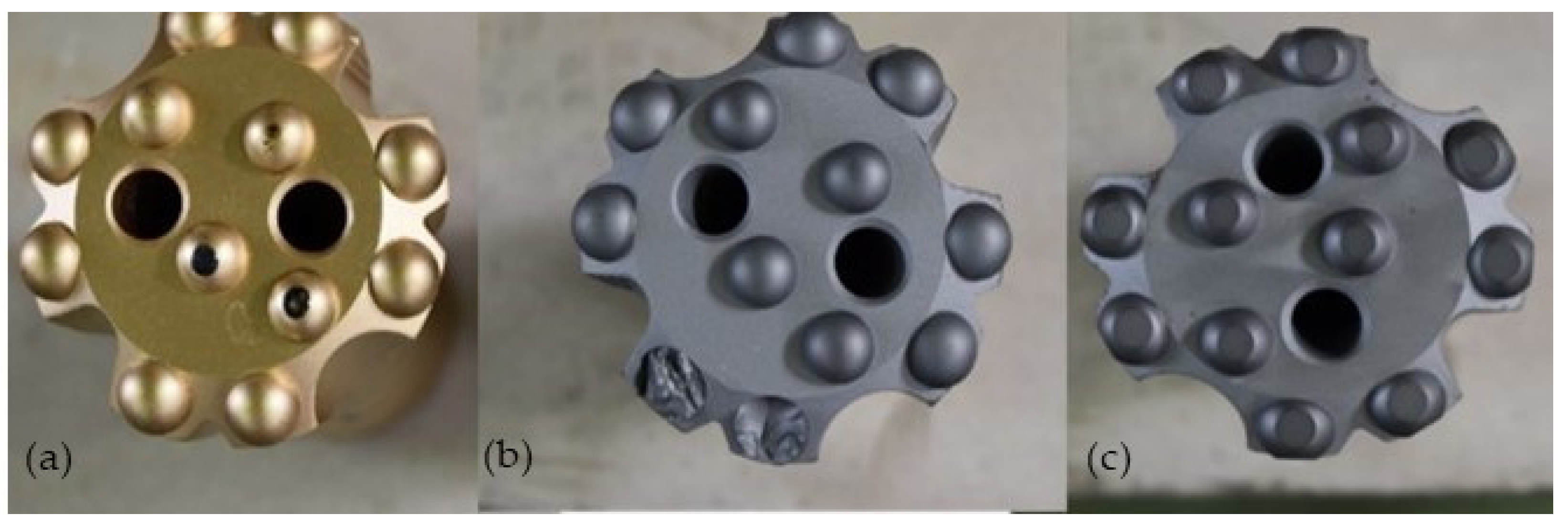
| Defective | Chipped button | 10 | 3120 | 1 | 60 |
| Abrasion | Worn out | 10 | 3120 | 1 | 60 |
| High impact pressure | Normal | 10 | 3120 | 1 | 60 |
| Misdirection | Normal | 10 | 3120 | 1 | 60 |
| Drill Length (m) | Impact Pressure (MPa) | Striking Frequency (Hz) | Rotary Pressure (MPa) | Feed Pressure (MPa) | Sampling Frequency (kHz) |
|---|---|---|---|---|---|
| 1 | 13.5-7 | 52 | 4–6 | 4 | 50 |
| Hardware and Software | Characteristics |
|---|---|
| Memory | 16 Gb |
| Processor | Intel i7-8750H CPU @ 2.2 GHz |
| Graphics | NVIDIA GeForce GTX 1060 |
| Operating system | Windows 10, 64 bits |
| Layer Type | Number of Filters | Size of Filter | Stride Value | Output Size | Number of Trainable Parameters |
|---|---|---|---|---|---|
| Input | - | - | - | 1 × 3000 × 1 | 0 |
| Convolution | 128 | 1 × 751 × 1 | 2 | 1 × 1126 × 128 | 96,256 |
| Batch normalization | 128 | - | - | 1 × 1126 × 128 | 256 |
| Leaky ReLU | - | - | - | 1 × 1126 × 128 | 0 |
| Max pooling | 1 | 1 × 3 × 1 | 1 | 1 × 1122 × 128 | 0 |
| Convolution | 128 | 1 × 281 × 128 | 2 | 1 × 421 × 128 | 4,604,032 |
| Batch normalization | 128 | - | - | 1 × 421 × 128 | 256 |
| Leaky ReLU | - | - | - | 1 × 421 × 128 | 0 |
| Max pooling | 1 | 1 × 3 × 1 | 1 | 1 × 417 × 128 | 0 |
| Fully connected | - | - | - | 1 × 1 × 500 | 26,880,500 |
| Fully connected | - | - | - | 1 × 1 × 500 | 2505 |
| Softmax | - | - | - | 1 × 1 × 5 | 0 |
| Kernel Name | Size of the 1st Convolutional Layer | Size of the 2nd Convolutional Layer | Training Accuracy (%) | Validation Accuracy (%) |
|---|---|---|---|---|
| Kernel 1 | 3 | 3 | 82.81 | 51.96 |
| Kernel 2 | 5 | 3 | 74.22 | 54.15 |
| Kernel 3 | 5 | 5 | 75.00 | 63.67 |
| Kernel 4 | 7 | 5 | 63.28 | 61.17 |
| Kernel 5 | 7 | 7 | 64.06 | 58.65 |
| Kernel 6 | 11 | 7 | 72.66 | 66.52 |
| Kernel 7 | 11 | 11 | 82.03 | 68.12 |
| Kernel 8 | 751 | 281 | 93.75 | 87.78 |
| Pooling Size in 1st and 2nd Convolutional Layer | Pooling Strategy | Training Accuracy (%) | Validation Accuracy (%) |
|---|---|---|---|
| 2 | Max pooling | 97.78 | 88.71 |
| 3 | Max pooling | 97.66 | 89.50 |
| 4 | Max pooling | 97.66 | 88.59 |
| 5 | Max pooling | 94.53 | 89.04 |
| 7 | Max pooling | 93.75 | 86.68 |
| 1st Convolutional Layer | 2nd Convolutional Layer | Training Accuracy (%) | Validation Accuracy (%) | Time (min) |
|---|---|---|---|---|
| 32 | 64 | 99.22 | 86.81 | 415.09 |
| 64 | 128 | 93.75 | 87.24 | 426.54 |
| 128 | 128 | 96.09 | 89.02 | 428.50 |
| 128 | 264 | 96.88 | 87.88 | 452.30 |
| Model | Training Accuracy (%) | Validation Accuracy (%) |
|---|---|---|
| DBFD 2 | 96.02 | 89.02 |
| DBFD 3 | 94.53 | 88.49 |
| DBFD 4 | 96.87 | 88.94 |
| Model | Classification Accuracy (%) | Time (min) | Learnable Parameters |
|---|---|---|---|
| Proposed DBFD | 88.7 | 428.50 | 31,515,805 |
| MLP | 54.7 | 170.52 | 2,003,002 |
| FCN | 76.7 | 476.57 | 167,558 |
| ResNet50 | 81.6 | 1805.29 | 16,185,685 |
Publisher’s Note: MDPI stays neutral with regard to jurisdictional claims in published maps and institutional affiliations. |
© 2021 by the authors. Licensee MDPI, Basel, Switzerland. This article is an open access article distributed under the terms and conditions of the Creative Commons Attribution (CC BY) license (https://creativecommons.org/licenses/by/4.0/).
Share and Cite
Senjoba, L.; Sasaki, J.; Kosugi, Y.; Toriya, H.; Hisada, M.; Kawamura, Y. One-Dimensional Convolutional Neural Network for Drill Bit Failure Detection in Rotary Percussion Drilling. Mining 2021, 1, 297-314. https://doi.org/10.3390/mining1030019
Senjoba L, Sasaki J, Kosugi Y, Toriya H, Hisada M, Kawamura Y. One-Dimensional Convolutional Neural Network for Drill Bit Failure Detection in Rotary Percussion Drilling. Mining. 2021; 1(3):297-314. https://doi.org/10.3390/mining1030019
Chicago/Turabian StyleSenjoba, Lesego, Jo Sasaki, Yoshino Kosugi, Hisatoshi Toriya, Masaya Hisada, and Youhei Kawamura. 2021. "One-Dimensional Convolutional Neural Network for Drill Bit Failure Detection in Rotary Percussion Drilling" Mining 1, no. 3: 297-314. https://doi.org/10.3390/mining1030019
APA StyleSenjoba, L., Sasaki, J., Kosugi, Y., Toriya, H., Hisada, M., & Kawamura, Y. (2021). One-Dimensional Convolutional Neural Network for Drill Bit Failure Detection in Rotary Percussion Drilling. Mining, 1(3), 297-314. https://doi.org/10.3390/mining1030019