A Unified Fractal Processing Framework for Normalized AIS and ECDIS Ship Trajectories

Abstract

The article presents a unified fractal approach to processing and analyzing ship trajectories based on AIS and ECDIS data. A comprehensive algorithmic pipeline is proposed, which provides time normalization, coordinate transformation, calculation of dynamic motion characteristics, and application of fractal analysis in sliding windows. This approach allows for the stable calculation of key parameters (course, angular velocity, deviation from the route) and detection of local changes in movement complexity that are not recorded by classical methods. The fractal indicators used (Higuchi, Katz, Petrosyan, DFA dimensions) demonstrate high reproducibility and resistance to typical navigation data shortcomings. The proposed framework is primarily intended for onboard and post-voyage analysis, supporting navigational performance assessment, trajectory reconstruction, and detailed investigation of vessel motion dynamics based on the records from AIS and ECDIS.

1. Introduction

The rapid growth of maritime traffic and the widespread deployment of Automatic Identification System (AIS) and Electronic Chart Display and Information System (ECDIS) technologies have led to the accumulation of large volumes of vessel trajectory data. These data streams provide a valuable basis for studying navigational processes, motion dynamics, and traffic patterns. However, raw AIS and ECDIS data are characterized by significant heterogeneity, irregular sampling rates, missing values, coordinate inconsistencies, and sensor-induced noise, which substantially limit their direct applicability for quantitative analysis and modelling.

In practical applications, vessel trajectory data are often collected from multiple sources with different temporal resolutions, reference coordinate systems, and data completeness levels. As a result, unprocessed trajectories frequently exhibit distortions in speed, course, and rotational parameters, making conventional kinematic or statistical analyses unreliable. This issue becomes particularly critical when higher-order motion characteristics are required, such as trajectory complexity, stability, or long-range temporal dependencies. Consequently, there is a strong need for a robust and reproducible preprocessing framework that transforms heterogeneous AIS/ECDIS records into analysis-ready representations.

Current scientific studies focus mainly on techniques for cleaning, rescaling, traffic index prediction, and trajectory interpolation. Generally, the bulk of the techniques are aimed at establishing measures that resemble more traditional metrics; that is, the speed profiles, route similarity, and traffic density estimates. At the same time, serious preparedness is hardly taken into account regarding requirements in terms of advanced traffic analytical approaches, especially those that employ nonlinear dynamics and fractal geometry. Noise removal as well as some temporal consistency and trajectory’s structure preservation need to be considered meticulously if the two methodologies are to be integrated. Should there be a lack of consistency among the methods in operation, naturally, the fractal metrics, deployed directly on raw data, give generally unstable or conflicting results.

Fractal analysis has proven to be an effective tool for describing the dynamics of complex systems, including motion trajectories. Metrics such as the Higuchi fractal dimension, detrended fluctuation analysis (DFA), Katz and Petrosyan dimensions, and box-counting methods allow for the quantitative assessment of motion complexity at different time scales. When applied to marine trajectories, these indicators reveal internal structural characteristics that are not captured by traditional kinematic descriptions. However, the reliability of fractal indicators depends largely on data normalization procedures, the choice of analysis windows, and the consistency of parameter values—aspects that are often overlooked in existing studies.

The literature studied on the research topic forms an interdisciplinary scientific basis for the development of a unified fractal structure for processing normalised ship trajectories derived from AIS and ECDIS data. At a fundamental level, fractal theory has proven effective for describing complex spatio-temporal structures characterised by irregularity, scale invariance, and hierarchical organisation in technical and natural systems, including architectural perception, antenna systems, geological structures, and uncertainty modelling [1,2,3,4,5]. Such properties are intrinsic to vessel trajectories, which emerge from the interaction of navigational decisions, environmental constraints, and operational regimes.

A significant number of studies focus on the quantitative description of complexity in spatial and temporal patterns using fractal dimension, multifractal spectra, Kolmogorov complexity, and Hurst-based indicators. These approaches have been successfully applied in land-use dynamics, material microstructures, geological formations, porous media, and energy-related processes, demonstrating their robustness for analysing non-stationary and nonlinear systems [3,6,7,8,9,10,11,12,13]. The ability of these measures to capture scale-dependent heterogeneity directly supports their applicability to AIS trajectories, where point density, curvature, and motion regimes vary over time.

Further evidence of the versatility of fractal metrics is provided by research in coal reservoirs, concrete materials, capillary transport systems, and permeability evolution, where fractal parameters are explicitly linked to transport properties, damage accumulation, and flow behaviour [14,15,16,17,18,19,20,21]. These findings reinforce the relevance of fractal representations for ship trajectories, which similarly reflect underlying transport processes and constraints imposed by navigation channels, traffic separation schemes, and port approaches.

A separate and methodologically important group of studies addresses signal, image, and time-series processing. Wavelet-based techniques, spectral methods, fractal–fractional operators, and image analysis algorithms are widely used for multi-scale decomposition, denoising, and feature extraction in acoustic signals, biomedical recordings, image quality assessment, and remote sensing imagery [22,23,24,25,26,27,28,29,30]. In the context of AIS and ECDIS data, these methods provide the mathematical basis for trajectory smoothing, temporal normalisation, anomaly suppression, and scale-consistent representation under irregular sampling and measurement conditions.

Recent works combining wavelet analysis with maritime, engineering, and thermal monitoring applications further highlight the potential of these methods for complex operational data and heterogeneous sensor streams [31,32]. Their integration with fractal analysis enables the construction of hybrid multi-resolution descriptors capable of preserving both global trajectory structure and local manoeuvring behaviour.

Research on ship motion analysis, trajectory pattern recognition, and maritime safety demonstrates that geometric, topological, and shape-based features of vessel paths carry critical information about manoeuvres, behavioural changes, traffic interactions, and navigational risk [33,34,35,36,37,38]. Studies focusing on ECDIS-related incidents and grounding accidents further confirm the importance of trajectory interpretation for safety assessment, situational awareness, and decision support [39].

In parallel, investigations into intelligent data processing, optimisation, and machine learning in safety-critical and transport domains show that fractal features can serve as stable, scale-invariant descriptors for classification, clustering, semantic analysis, and optimisation of complex dynamic systems [40,41,42,43,44,45,46,47,48]. These properties are particularly valuable for maritime applications, where trajectory data must be compared across different spatial scales, traffic densities, and operational contexts, including urban, port, and offshore environments [47,49,50].

Complementary studies addressing shipboard technical systems, propulsion efficiency, energy storage, refrigeration cycles, and operational performance further support the feasibility of linking trajectory behaviour with technical, energetic, and mechanical states of vessels and transport systems [51,52,53,54,55,56,57,58,59]. Such integration is essential for moving from descriptive trajectory analysis toward decision-support, risk-oriented navigation, and system-level maritime safety frameworks.

The reviewed literature basis confirms the maturity of fractal and multiscale analysis methods across diverse application domains while simultaneously revealing a clear methodological gap. Despite the demonstrated effectiveness of fractal metrics, wavelet techniques, and shape-based descriptors, no unified framework currently exists for the normalised fractal processing of AIS and ECDIS ship trajectories that consistently integrates preprocessing, multi-scale feature extraction, geometric interpretation, and decision-support integration within a single coherent methodology.

Despite the growing interest in applying nonlinear and fractal methods to navigational data, the literature lacks a comprehensive and reproducible processing pipeline that systematically integrates AIS/ECDIS data normalization with sliding-window fractal analysis. Most existing works focus either on isolated preprocessing steps or on specific analytical outcomes, without providing an end-to-end methodological framework. This gap limits reproducibility, cross-study comparability, and the practical transferability of advanced trajectory analysis methods. Thus, despite the significant volume of scientific work in the fields of AIS/ECDIS trajectory analysis and fractal methods, the problem of creating a unified, reproducible, and parametrically controlled data-processing pipeline that combines trajectory normalization with sliding fractal analysis remains unresolved. This study examines the elimination of this methodological gap.

The objective of this study is to develop a unified fractal processing pipeline for converting AIS and ECDIS vessel trajectory data to stable, fractal-ready representations. The proposed pipeline comprises time normalization, coordinate system identification and projection, derivation of dynamic motion parameters, a sliding window segmentation, and a multi-metric fractal computation. This description underlines the importance of reproducibility, parameter transparency, and computational robustness in this regard. The framework resulting from this process will provide a structured base for further analytical tasks, allowing a consistent study of vessel motion dynamics by fractal indicators.

To achieve this goal, the study addresses the following objectives: analyzing the structure of AIS/ECDIS trajectory data and developing a universal procedure for automated reading and normalization of trajectories with different coordinate and time formats, converting them into a unified metric system S^(k) = {t_i, X_i, Y_i, COG_i, ROT_i, XTE_i} for each voyage. Additionally, it aims to construct a system of fractal and dynamic indicators that characterize the geometry and “roughness” of vessel motion within sliding windows. This includes the Higuchi, DFA, Katz, and Petrosian fractal dimensions for cross-track deviations XTE, along-track motion, and angular velocity, as well as the fractal dimension of the spatial path.

The proposed framework’s individual components, like trajectory normalization and fractal metrics, have already been investigated separately, but the originality of this work is in their organized merger into one single pipeline that is reproducible. More specifically, integrating automatic trajectory normalization with sliding-window multi-metric fractal analysis enables consistent comparison of different trajectories, which is not possible with ad hoc or standalone implementations. Hence, the contribution goes beyond refining metrics and offering a structured methodological framework for comparative maritime trajectory analysis.

It is important to stress that the proposed processing framework is not for real-time VTS operations at all, where ECDIS data may not be available. Rather, the use of ECDIS trajectories is most relevant and seen in onboard and post-voyage analytical contexts including navigational performance assessment, training, incident investigation, voyage reconstruction, and VDR-based analysis. It is in this context only that AIS and ECDIS data have been considered as complementary sources in the processing of a unified trajectory rather than parallel inputs for real-time traffic monitoring.

The remainder of this paper is organized as follows. Section 2 describes the data sources and the proposed trajectory processing methodology. Section 3 presents the obtained results and illustrative examples. Section 4 discusses the implications, limitations, and operational applicability of the proposed framework. Finally, Section 5 summarizes the main conclusions of the study.

2. Materials and Methods

In line with the paper’s aim, we proceed to a step-by-step description of how the stated objectives are achieved. The first task is a formal analysis of the structure of AIS/ECDIS trajectory data and the development of a universal procedure for automated reading and normalization of trajectories with different coordinate and time formats, converting them into a single metric system.

Let us introduce a unified metric representation of a vessel’s trajectory obtained from heterogeneous AIS/ECDIS files (t_i, X_i, Y_i, COG_i, ROT_i, XTE_i), which serves as the basis for subsequent fractal analysis.

2.1. Structure of AIS/ECDIS Trajectory Data

Formal Statement of the Normalization Problem

Let the input consist of a set of trajectory files

$$\mathcal{F}={\left\{F^{\left(k\right)}\right\}}_{k=1}^K,$$

(1)

where each file F^(k) corresponds to one voyage or one fragment of vessel motion, formally, the file F^(k) is a rectangular table $F^{\left(k\right)}=\left\{z_{i,j}^{\left(k\right)}|i=1,\dots ,N_k, j=1,\dots ,M_k\right\}$, where i is the record index (time sample) and j is the column index.

A typical i-row can be written as a vector $z_i^{\left(k\right)}=\left({\mathrm{Time}}_i, {\mathrm{Lat}}_i, {\mathrm{Lon}}_i, {\mathrm{COG}}_i, {\mathrm{SOG}}_i,\dots \right)$, whose components may be missing, expressed in different units of measurement and stored in various formats (numeric, textual, DMS, Excel time, etc.).

In this study, the rate of turn is treated as the rate of change of heading (HDG). When AIS-derived COG is used as a proxy due to data availability, this approximation is explicitly acknowledged and its limitations are discussed.

The goal of normalization is to construct a mapping

$$\mathcal{N}:F^{\left(k\right)}\to S^{\left(k\right)},$$

(2)

where S^(k) is a standardized time series in a unified metric system

$$S^{\left(k\right)}={\left\{\left(t_i, x_i, y_i, {\mathrm{COG}}_i, {\mathrm{ROT}}_i, {\mathrm{XTE}}_i, {\phi }_i, {\lambda }_i\right)\right\}}_{i=1}^{N_k^{*}}.$$

(3)

Here t_i—time in seconds from the start of the trajectory (t₁ = 0); (x_i, y_i)—coordinates in metres in a local Cartesian system; COG_i—true course of the vessel (degrees); ROT_i = dCOG/dt—angular turning rate (deg/s); XTE_i—cross-track error with respect to the smoothed trajectory (m); φ_i, λ_i—latitude and longitude in decimal degrees (if available in the raw data).

Thus, the normalization problem reduces to constructing two mappings:

-

Temporal unification ${\mathrm{\Phi }}_t:{\mathrm{Time}}_i\to t_i\in ℝ, t_i\left(\sec \right)$;

-

Spatial unification ${\mathrm{\Phi }}_{xy}:\left({\mathrm{Lat}}_i, {\mathrm{Lon}}_i\right) or \left(X_i, Y_i\right) \to \left(x_i, y_i\right)\in {ℝ}^2$.

The implemented software pipeline automatically performs:

-

Reading CSV/XLS/XLSX files into a unified tabular DataFrame format;

-

Detection of service columns (time, latitude, longitude, course, speed);

-

Identification of the geocoordinate format (decimal degrees, DMS, already metric X/Y);

-

Conversion of coordinates into metres using the EPSG:32635 projection or a local pseudo-Mercator approximation;

-

Conversion of time into seconds and estimation of the sampling step Δt;

-

Construction of the normalized trajectory series S^(k).

2.2. Automated Reading of Tables and Detection of Service Columns

2.2.1. Universal File Reading

The read_any(path)algorithm implements a universal import mechanism. Suppose the file extension is .csv, the call pd.read_csv(path, encoding=“utf-8”, sep=None, engine=“python”) is used with automatic delimiter detection.

If the file is an Excel workbook (.xls, .xlsx), all sheets sheet_name are scanned sequentially:

-

For the first H rows of each sheet (in the code H = 10), a candidate header row

h_r = (h_r,1, … , h_{r, M}) is formed and normalized (lowercase, trimmed);

-

If any element of h_r contains the keywords {lat, lon, time, utc, lat, long, time, date}, this row is accepted as the header, and the sheet is read as df = read_excel(sheet, header = r);

-

If none of the top rows contains the keywords, the sheet is read with the default header and checked for non-emptiness.

Thus, over the set of possible header-format variants, we construct an operator R: “file → DataFrame” that is robust to changes in the structure of xls/xlsx files (different sheets, header rows, presence of service rows at the top).

2.2.2. Detection of Service Columns

After importing a DataFrame D with the set of columns C = {c₁, …, c_M}, the function detect_columns(df) is applied, which builds a mapping from the physical columns to their semantic roles (latitude, longitude, time, course, speed, etc.) $\mathrm{\Psi }:\mathcal{C}\to \left\{\mathrm{lat}, \mathrm{lon}, \mathrm{time}, \mathrm{cog}, \mathrm{sog}\right\}\cup \left\{\varnothing \right\}$.

Normalization of column names is implemented by the function: norm(c) = lowercase(trim(replace_nbsp(c))),after which a mapping from the original names to the normalized ones is created ${\mathcal{C}}_{\mathrm{norm}}=\left\{\mathrm{norm}\left(c_j\right)\to c_j\right\}$.

For each type of service column a list of keywords is specified, for example:

-

For latitude: K_lat = {“lat”, “latitude”};

-

For longitude: K_lon = {“lon”, “long”, “longitude”};

-

For time: K_t = {“time”, “timestamp”, “utc”, “datetime”, “date”}, etc.

The column-selection operator checks for the presence of at least one keyword from the corresponding set in the normalized header and returns the matching column name (or index)

$$\mathrm{pick}\left(\mathcal{K}\right)=\left\{\begin{array}{l}\mathrm{the} \mathrm{first} с\in {\mathcal{C}}_{norm}, \mathrm{for} \mathrm{which} \exists kw\in \mathcal{K}:kw\subset norm\left(c\right),\\ \varnothing , \mathrm{if} \mathrm{there} \mathrm{are} \mathrm{none}.\end{array}\right.$$

(4)

Thus, for example, the latitude column is determined as the column whose normalized header contains an element from ${\mathcal{K}}_{lat}$:

$$c_{lat}=\mathrm{pick}\left({\mathcal{K}}_{lat}\right) абo {\mathcal{C}}_{norm}\left["lat"\right].$$

(5)

At the output we obtain the tuple (c_lat, c_lon, c_t, c_cog, c_sog), which is then passed to the georeferencing and normalization procedure.

In this way the format of geocoordinates is automatically identified and DMS values are parsed into decimal degrees.

To support both decimal and DMS formats (e.g., 41°02′30″ N), a regular expression DMS_RE is used to extract deg, min, sec, hem ∈ {N, S, E, W}, after which latitude/longitude in decimal degrees are computed as

$$\phi =s\cdot \left(\left|\mathrm{deg}\right|+{\displaystyle \frac{\min }{60}}+{\displaystyle \frac{\sec }{3600}}\right), \mathrm{where} \mathrm{the} \mathrm{sign} \mathrm{is} s=\left\{\begin{array}{l}-1, \mathrm{hem}\in \left\{S, W\right\},\\ +1, else.\end{array}\right.$$

(6)

This formula is implemented in parse_dms_value() and vectorised in parse_dms_series().

2.2.3. Detection of the Type of Geodata (detect_or_guess_geo)

The function detect_or_guess_geo(df) builds a dictionary geo = {mode, lat, lon} or geo = {mode, x, y}, where mode ∈ {latlon_decimal, latlon_dms, latlon_decimal_guess, latlon_dms_guess, xy}.

2.3. Logical Predicates of the Functions

2.3.1. Explicit LAT/LON Column Names

If there exist columns c_lat, c_lon, whose names contain keywords such as “lat” and “lon”, then the vectors v_lat = to_float(c_lat), v_lon = to_float(c_lon) are computed, where to_float_series performs normalization of string values and their conversion to numeric form. If share_notna(v_lat) > 0.4 and share_notna(v_lon) > 0.4, the mode is set to mode = mode=“latlon_decimal”.

Otherwise, DMS parsing is attempted: v_lat = parse_dms_series(c_lat), v_lon = parse_dms_series(c_lon), and, under the same completeness conditions, the mode is set to mode=“latlon_dms”.

2.3.2. Explicit Metric X/Y

Columns with names of the form x_m, east, easting, y_m, north, northing are searched for. If the median of ∣x∣ or ∣y∣ exceeds 1000 m, the mode is set to mode=“xy” with references to the corresponding columns.

2.3.3. Identification of Numeric Candidates for lat/lon

A list of numeric columns (c,v_c) is formed. Candidates for latitude are those for which share_notna(v_c) > 0.5, share(v_c ∈ [−90, 90]) > 0.8. Among the candidates, the columns with the maximum variance $c_{lat}=\arg \underset{c\in LatCand}{\max }\sigma \left(v_c\right), c_{lon}=\arg \underset{c\in LonCand}{\max }\sigma \left(v_c\right)$. If c_lat ≠ c_lon, the mode is set to mode=“latlon_decimal_guess”.

2.4. DMS Candidates for lat/lon

For each column, DMS parsing is attempted and the resulting values are checked for belonging to the ranges [−90, 90] and [−180, 180]. In the presence of at least one valid (lat, lon) pair, the mode is set to mode=“latlon_dms_guess”. If none of the variants succeed, an explicit error “Could not detect coordinates” is raised, which guarantees explicit detection of anomalous files.

2.4.1. Transformation of Geographic Coordinates into a Metric System

The function to_xy(lat, lon) implements the mapping ${\mathrm{\Phi }}_{xy}:\left({\phi }_i, {\lambda }_i\right)\to \left(x_i, y_i\right)$.

2.4.2. Main Mode (Pyproj Available)

If the pyproj package is installed, the projection $\left(x_i, y_i\right)=P\left({\phi }_i, {\lambda }_i\right)$ is used, where

P:EPSG:4326→EPSG:32635, P=Transformer.from_crs(“EPSG:4326”,”EPSG:32635”, always_xy=True).

This yields metric coordinates in the UTM zone 35N system, which is adequate for the Bosphorus region and Black Sea waters.

2.4.3. Mode Without Pyproj (Local Pseudo-Mercator Approximation)

The median latitude φ₀ = median φ_i is computed, after which classical approximations for metres per degree of latitude and longitude are used:

$$\begin{array}{l}{m}_{\mathrm{lat}}=\mathrm{111,132.954}-559.822\cos \left(2{\phi }_0\right)+1.175\cos \left(4{\phi }_0\right),\\ m_{\mathrm{lon}}=\mathrm{111,132.954}\cos \left({\phi }_0\right),\\ x_i=\left({\lambda }_i-{\lambda }_{\min }\right)\cdot m_{\mathrm{lon}}, y_i=\left({\phi }_i-{\phi }_{\min }\right)\cdot m_{\mathrm{lat}},\end{array}$$

(7)

where λ_min = min_i λ_i, φ_min = min_iφ_i.

Such a local coordinate system is conveniently centred in the area of the route and provides correct distances in metres for relative trajectory analysis.

2.5. Unification of the Time Axis and Estimation of the Sampling Step

2.5.1. Selection of the Time Column

The time column ctc_tct is determined by the detect_columns function and passed to estimate_dt(df, tcol), which constructs the mapping ${\mathrm{\Phi }}_t:c_t\to \left(t_1,\dots ,t_N\right), t_1=0, t_{i+1}-t_i=\Delta t$.

2.5.2. Estimation of Δt from Different Time Formats

The auxiliary function safe_median_diff(a) = median({a_i+1 − a_i}_i) computes the median difference between consecutive values (after discarding NaNs) and is used to estimate the sampling step.

2.5.3. Algorithm of the Function: Textual “HH:MM:SS” Format

The column is converted into Timedelta: τ_i = to_timedelta(s_i), then the array is mapped to seconds, and the median difference $\Delta t=safe\_median\_diff\left(t_i^{\left(\sec \right)}\right)$.

For full date-time (datetime) format an analogous procedure is applied—$d_i=\mathrm{to}\_\mathrm{datatime}\left(s_i\right), \Delta t=\mathrm{median}\left(t_{i+1}^{\left(\sec \right)}-t_i^{\left(\sec \right)}\right)$—with the same range check.

2.5.4. Numeric Representations

If to_numeric succeeds, the median difference m_d = median(n_i+1 − n_i) is computed, after which a sequential interpretation is applied:

Excel day fraction: if 1 × 10⁻⁶ ≤ m_d ≤ 1 × 10⁻³, Δt = m_d · 86,400, 0.05 ≤ Δt ≤ 10 ⇒ this value is accepted:

-

Direct seconds: If 0.05 ≤ m_d ≤ 10, we set Δt = m_d;

-

Milliseconds: If 50 ≤ m_d ≤ 2000, Δt = m_d/1000;

-

Default value: If none of the regimes yield a valid Δt in the range [0.05;10] s, the default value Δt = 1.0 s is used.

After estimating Δt, a relative time scale is constructed t_i = (i − 1) Δt, i = 1, …, N, which is used in the computation of velocities, fractal indicators, and in sliding-window processing.

2.6. Construction of the Normalized Trajectory Series

The function derive_series_auto(df, tcol, cog_col, sog_col, lat_hint, lon_hint) combines the operators Φ_t and Φ_xy described above and forms the basic time series.

2.6.1. Obtaining Metric Coordinates

According to geo[“mode”]:

if the mode starts with “latlon”, the raw columns are converted to decimal degrees (via to_float_series or parse_dms_series), after which Φ_xy is applied to obtain X_i,Y_i;

if mode=“xy”, the numeric values of the columns X, Y are taken directly.

2.6.2. Generalization of the Course over Ground (COG)

If a course column is present, the vector COG_i (in degrees) is formed directly. Otherwise, the course is computed from the coordinate derivatives, e.g.,

$$v_i^x={\displaystyle \frac{d{x}_i}{dt}}, v_i^y={\displaystyle \frac{d{y}_i}{dt}}, CO{G}_i=\left({\displaystyle \frac{180}{\pi }}\arctan 2\left(v_i^x, v_i^y\right)+360\right)\mathrm{mod}360.$$

(8)

2.6.3. Course Unwrapping (Removal of 0°/360° Jumps)

A standard phase-unwrapping operation is used—${\mathrm{COG}}_i^u=\mathrm{unwrap}\left({\mathrm{COG}}_i\right)$—where unwrap is applied in radians with subsequent conversion back to degrees (via np.unwrap). Angle unwrapping is applied to avoid jumps near 360° and to ensure correct computation of derivatives and ROT.

2.6.4. Angular Rate of Turn (ROT)

The angular rate of turn is computed as a numerical derivative:

$${\mathrm{ROT}}_i\approx {\displaystyle \frac{{\mathrm{COG}}_{i+1}^u-{\mathrm{COG}}_{i-1}^u}{2\Delta t}},$$

(9)

which in the code is implemented as np.gradient(cog_u)/dt.

2.6.5. Cross-Track Error with Respect to the Smoothed Trajectory (XTE)

Define the smoothed trajectory as ${\tilde{x}}_i=\mathrm{smooth}\left(x_i, \mathrm{win}\right), {\tilde{y}}_i=\mathrm{smooth}\left(y_i, \mathrm{win}\right)$, where smooth_series is a moving average with window win = 51.

The derivatives of the smoothed path are estimated as

$$d{\tilde{x}}_i={\displaystyle \frac{d\tilde{x}}{dt}}, d{\tilde{y}}_i={\displaystyle \frac{d\tilde{y}}{dt}},$$

(10)

and the tangent vector is normalized

$$t_i={\displaystyle \frac{1}{\sqrt{d{\tilde{x}}_i^2+d{\tilde{y}}_i^2+\epsilon }}}\left(d{\tilde{x}}_i, d{\tilde{y}}_i\right),$$

(11)

after which the oriented normal vector is defined as $n_i=\left(-t_i^y, t_i^x\right)$.

Deviation vector and cross-track error $\Delta r_i=\left(x_i-{\tilde{x}}_i, y_i-{\tilde{y}}_i\right)$. The deviation vector of the actual point from the smoothed path is ${\mathrm{XTE}}_i=〈\Delta r_i, n_i〉=\left(x_i-{\tilde{x}}_i\right)n_i^x+\left(y_i-{\tilde{y}}_i\right)n_i^y$. Then the cross-track error (XTE) is computed as the scalar product.

2.7. Formation of the Normalized Table

For each file, a DataFrame $\mathrm{norm}={\left[t_i, X_i, Y_i, {\mathrm{COG}}_i^u, {\mathrm{ROT}}_i {\mathrm{XTE}}_i\right]}_{i=1}^N$ is constructed, with optional additional columns LAT, LON when geographic coordinates are available.

This table is saved in the form <input_filename>_normalized.csv, i.e., one normalized file per input trajectory.

For each file an additional summary record is formed (in the file fractal_report.csv), where the following are stored: n_points, dt_sec, mode_geo, and the global fractal metrics (Higuchi, DFA, Katz, Petrosian, FD_path_2D) for the series COG, ROT, XTE.

2.8. Data Provenance and Preprocessing Effects

It is well known that both AIS and ECDIS trajectory data are primarily derived from GNSS measurements that have already undergone sensor-level filtering, including Kalman smoothing. The aim of the processing framework is not to smooth the trajectory geometry further, but rather to temporalize normality and metric constancy. The framework attempts to ensure that high-frequency maneuvering dynamics will not be affected by resampling and interpolation. Specifically, the applicable analysis leads to constraint on the fractal metrics due to the actual time interval problem in AIS data sets, whereas observed stability regarding some metrics should be understood on their own, coming from pre-filtering. Therefore, these limitations prohibit the utilization of this method. This is once more spelled out in the prose below the platea.

2.9. Formation of a System of Fractal and Dynamic Indicators in Sliding Windows

Sliding-Window Model

Let, after normalization, we have the discrete time series

$$\begin{array}{l}X={\left\{X_i\right\}}_{i=1}^N, Y={\left\{Y_i\right\}}_{i=1}^N,\\ XTE={\left\{{\mathrm{XTE}}_i\right\}}_{i=1}^N, \theta ={\left\{{\mathrm{COG}}_i\right\}}_{i=1}^N, \omega ={\left\{{\mathrm{ROT}}_i\right\}}_{i=1}^N\end{array},$$

(12)

where t_i = (i − 1)Δt is time in seconds (sampling in seconds), and Δt is the discretisation step obtained by the procedure estimate_dt(). The step Δt is estimated as the median of the differences t_i and is minimally sensitive to outliers.

In the code, the sliding-window parameters are specified as T_w = WINDOW_SEC = 120 s, T_s = STEP_SEC = 10 s.

$$f_s={\displaystyle \frac{1}{\Delta t}}, L=⌊T_w{f}_s⌋, S=⌊T_s{f}_s⌋,$$

(13)

which correspond to the window duration and the window shift in seconds, respectively.

Let L be the window length in points and S be the window shift in points. Then the j-th window (analysis episode) corresponds to the index interval

I_j = {n_j, n_j+1, …, n_j + L − 1}, n_j = 1+(j−1)S,

$$i=1,\dots ,M, M=⌊{\displaystyle \frac{N-L}{S}}⌋+1.$$

(14)

In other words, the window is shifted along the trajectory by S samples at each step.

For each window, the local signal fragments are extracted, for example, for cross-track error

$$\begin{array}{l}{x}^j=\left\{{\mathrm{XTE}}_i|i\in I_j\right\}, {\omega }^j=\left\{{\mathrm{ROT}}_i|i\in I_j\right\},\\ r^j=\left\{\left(X_i, Y_i\right)|i\in I_j\right\},\end{array}$$

(15)

and, if necessary, analogous fragments can be formed for COG_i, ROT_i, or other derived series.

In the current implementation the sliding fractal metrics are computed for x^j (cross-track deviations XTE), whereas the global indicators are evaluated for θ, ω, XTE, and the spatial path r. The algorithm is easily extensible to along-track motion (YTE) and to ω in sliding windows using the same functions.

The function sliding_metrics(ts, fs, window_sec, step_sec, metric_fn)in the code formally implements the operator

$$\begin{array}{l} S_{\mathrm{metric}}:{\left\{x_i\right\}}_{i=1}^N\to {\left\{\left(t_0^j, m^j\right)\right\}}_{j=1}^M,\\ t_0^t=\left(n_j-1\right)\Delta t, m^j=\mathrm{metric}\_\mathrm{fn}\left({\left\{x_i\right\}}_{i\in I_j}\right).\end{array}$$

(16)

2.10. Higuchi Fractal Dimension for a Scalar Process

For each scalar series ${\left\{x_i\right\}}_{i=0}^{N-1}\left(\mathrm{COG}, \mathrm{ROT}, \mathrm{XTE}\right)$ the Higuchi fractal dimension D_H is calculated according to the classical Higuchi scheme. For each scale k = 2, …, k_max (у кoді k_max = 16) k subsequences are constructed

$$X_m^k=\left\{x_m, x_{m+k}, x_{m+2k},\dots \right\}, m=0,1,\dots ,k-1.$$

(17)

For each subsequence the “length” of the polyline is estimated:

$$L_m\left(k\right)={\displaystyle \frac{N-1}{⌊\frac{N-m-1}{k}⌋k}}{\displaystyle \sum _{j=1}^{⌊\frac{N-m-1}{k}⌋}\left|x_{m+jk}-x_{m+\left(j-1\right)k}\right|}.$$

(18)

Intuitively, this formulation captures the rate at which trajectory complexity evolves across successive temporal scales, allowing local structural changes in vessel motion to be quantified.

The average length for scale k is

$$L\left(k\right)={\displaystyle \frac{1}{\left|{\mathcal{M}}_k\right|}}{\displaystyle \sum _{m\in {\mathcal{M}}_k}{L}_m\left(k\right)},$$

(19)

where ${\mathcal{M}}_k$ is the set of indices m for which the corresponding subsequence is non-empty $X_m^k\ge 2$. For a series with fractal structure the following power–law relation holds

$$L\left(k\right)\sim C{k}^{-D_H}.$$

(20)

In logarithmic scale:

$$\ln L\left(k\right)\approx \ln C-D_H\ln k.$$

(21)

The implemented function higuchi_fd(ts) forms the array of pairs (ln k, ln L(k)), performs linear regression by the least squares method, and returns the estimate of the fractal dimension

$$D_H=-{\widehat{\beta }}_1, {\widehat{\beta }}_1=\arg \underset{{\beta }_0,{\beta }_1}{\min }{\displaystyle \sum _k{\left(\ln L\left(k\right)-{\beta }_0-{\beta }_1\ln k\right)}^2}.$$

(22)

In our case global metrics $D_H^{\mathrm{COG}}=\mathrm{Higushi}\_\mathrm{COG}, D_H^{\mathrm{ROT}}=\mathrm{Higuchi}\_\mathrm{ROT}, D_H^{\mathrm{XTE}}=\mathrm{Higuchi}\_\mathrm{XTE}$, which are written to fractal_report.csv.

Sliding metrics for XTE

$$D_{H,j}^{\mathrm{XTE}}={\mathrm{Higuchi}\_\mathrm{XTE}}^j=D_H\left(x^j\right),$$

(23)

which form the column Higuchi_XTE in fractal_windows.csv with reference to the time t0_sec.

2.11. Detrended Fluctuation Analysis (α-Exponent)

To analyze scale-dependent fluctuations, the DFA method is used, implemented in the function dfa_alpha(ts). Let ${\left\{x_i\right\}}_{i=1}^N$ be the stationary series (COG, ROT, XTE). We construct the integrated profile:

$$y\left(j\right)={\displaystyle \sum _{i=1}^j\left(x_i-\overline{x}\right)}, j=1,\dots ,N,$$

(24)

where $\overline{x}$ is the mean value.

Next, we choose a set of scales s (in the code they are logarithmically spaced from min_win up to max_win_frac\cdot N), for each scale s we split the profile y(j) into n_s = ⌊N/s⌋ non-overlapping segments of length s. In each segment ν = 1, …, n_s we perform a linear regression

$$y\left(j\right)\approx a_{v}j+b_v, j\in \left[\left(v-1\right)s+1, vs\right],$$

(25)

and compute the deviations

$${\epsilon }_v\left(j\right)=y\left(j\right)-\left(a_{v}j+b_v\right).$$

(26)

The root-mean-square deviation for scale s is then

$$F^2\left(s\right)={\displaystyle \frac{1}{n_{s}s}}{\displaystyle \sum _{v=1}^{n_s}{\displaystyle \sum _{j=1}^s{\epsilon }_v{\left(j\right)}^2}}.$$

(27)

For a self-similar series, we have F(s)∼s^α, i.e., ln F(s) ≈ αlns + const. The function dfa_alpha(ts) returns the estimate $\widehat{\alpha }$ as the slope of the straight line on the lnF(s)—lns. Within the system of indicators:

-

Global values α^COG=DFA_COG, α^ROT = DFA_ROT, α^XTE = DFA_XTE;

-

Sliding values for XTE ${\alpha }_j^{\mathrm{XTE}}=DFA\_XT{E}^j=\mathrm{dfa}\_\mathrm{alpha}\left(x^j\right)$, which are computed in moving windows.

2.12. Katz Fractal Dimension

The function katz_fd(ts) implements one of the classical indicators of the “roughness” of a curve. For a series ${\left\{x_i\right\}}_{i=1}^N$:

-

Total length of the trajectory:

$$L={\displaystyle \sum _{i=2}^N\left|x_i-x_{i-1}\right|}.$$

(28)

-

Maximum distance to the initial point:

$$d=\underset{1\le i\le N}{\max }\left|x_i-x_1\right|.$$

(29)

The Katz fractal dimension is defined as:

$$D_K={\displaystyle \frac{{\log }_{10}\left(N\right)}{{\log }_{10}\left(N\right)+{\log }_{10}\left(\frac{d}{L}\right)}}.$$

(30)

In the code, additional checks are provided for the cases L = 0 or d = 0 (in which case D_K = 1 is returned as a degenerate value). Its use within the programming framework is as follows:

-

Globally $D_K^{\mathrm{COG}}=\mathrm{Katz}\_\mathrm{COG}, D_K^{\mathrm{ROT}}=\mathrm{Katz}\_\mathrm{ROT}, D_K^{\mathrm{XTE}}=\mathrm{Katz}\_\mathrm{XTE},$ are written to fractal_report.csv;

-

Locally for XTE: $D_{K,j}^{\mathrm{XTE}}={\mathrm{Katz}\_\mathrm{XTE}}^j=D_K\left(x^j\right)$, form the Katz_XTE column in fractal_windows.csv.

This indicator is sensitive to “breakage” (irregularity) of the trajectory within the sliding window and is used in conjunction with Higuchi’s fractal dimension and DFA indicators to form a local fractal characteristic of the vessel’s movement.

2.13. Petrosian FD and Dynamic Characteristics of Angular Velocity

Although the problem statement focuses on Higuchi, DFA, and Katz, the code additionally implements the Petrosian FD as a fast indicator of chaos for COG, ROT, and XTE:

$$D_P={\displaystyle \frac{{\log }_{10}\left(N\right)}{{\log }_{10}\left(N\right)+{\log }_{10}\left(\frac{N}{N+0.4N_{\delta }}\right)}},$$

(31)

where N_δ is the number of sign changes in the first difference Δx_i = x_i − x_i−1.

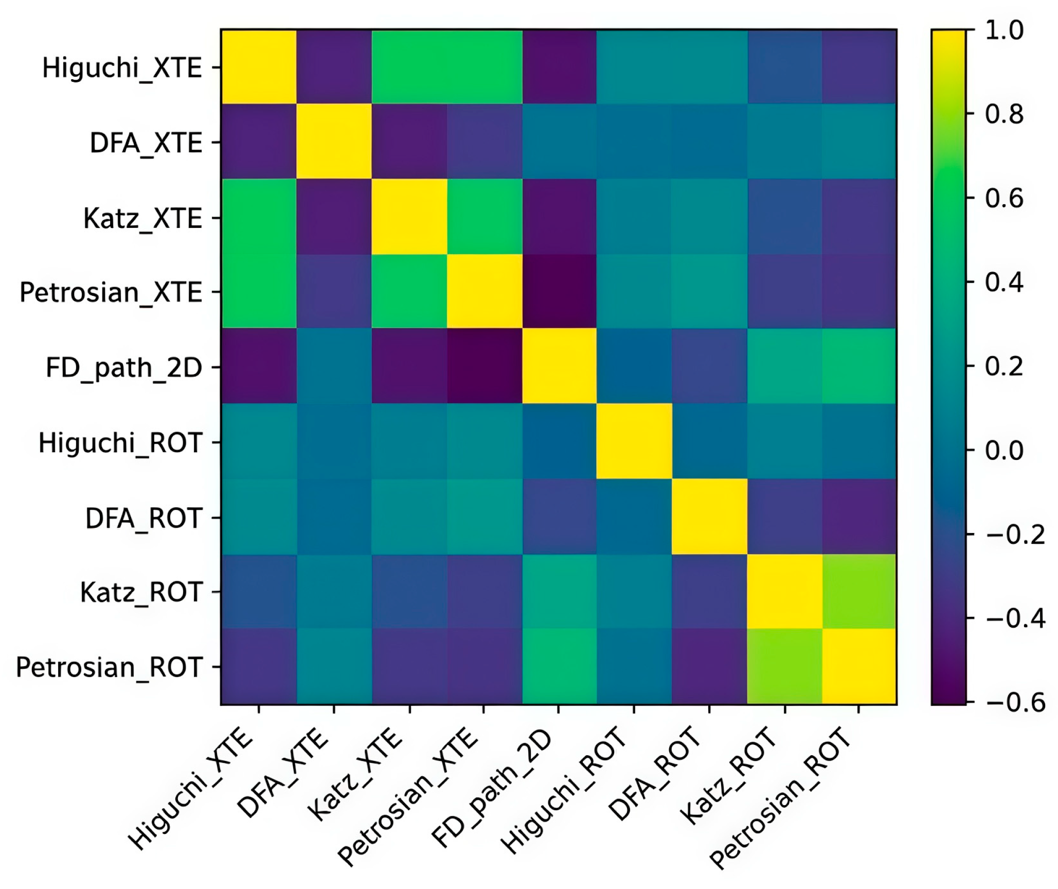
This indicator is included in fractal_report.csv as Petrosian_COG, Petrosian_ROT, Petrosian_XTE and is used at the stage of constructing the correlation matrix of fractal indicators. The dynamic indicators in the system are represented by the angular velocity itself ω = ROT(t), obtained as the numerical derivative of COG(t); subsequent episodic statistics (mean value, maximum, and standard deviation of ∣ROT∣ over time intervals), which are computed at the next stage (function rot_stats_in_range()) and interpreted as dynamic characteristics of the “aggressiveness” of maneuvering.

Thus, the fractal indicators (Higuchi, DFA, Katz, Petrosian) describe the geometric complexity of the signals XTE, COG, ROT, whereas ROT and its statistics characterize the dynamics of control (speed and variability of turns).

2.14. Fractal Dimension of the Spatial Vessel Path

For the spatial path $r={\left\{\left(X_i, Y_i\right)\right\}}_{i=1}^N$, the box-counting fractal dimension D_B is computed (function box_count_fd(X,Y)). The minimal square containing the trajectory is determined:

$$\begin{array}{l}{x}_{\min }=\underset{i}{\min }{X}_i, x_{\max }=\underset{i}{\max }{X}_i, y_{\min }=\underset{i}{\min }{Y}_i, y_{\max }=\underset{i}{\max }{Y}_i,\\ L=\max \left(x_{\max }-x_{\min }, y_{\max }-y_{\min }\right).\end{array}$$

(32)

A set of scales is formed as ε_j = L/2^j, j = 1, …, J (in the code num_scales = 8).

For each scale ε_j, the plane is divided into a square grid with step ε_j, the trajectory points are quantised:

$${\xi }_i=⌊{\displaystyle \frac{X_i-x_{\min }}{{\epsilon }_j}}⌋, {\eta }_i=⌊{\displaystyle \frac{Y_i-y_{\min }}{{\epsilon }_j}}⌋,$$

(33)

and the number of occupied cells is computed: N(ε_j)=∣{(ξ_i,η_i)}∣.

According to fractal theory

$$N\left(\epsilon \right)\sim {\epsilon }^{-D_B}, \Rightarrow \ln N\left(\epsilon \right)\approx D_B\ln {\displaystyle \frac{1}{\epsilon }}+\mathrm{const}.$$

(34)

The function box_count_fd performs a regression of lnN(ε_j) on ln(1/ε_j) and returns the estimate DB=FD_path_2D, which is written to fractal_report.csv. Values of D_B close to 1 correspond to an “almost straight” trajectory, whereas an increase in D_B to 1.5–1.7 indicates pronounced jaggedness and loop-like behaviour of the path.

2.15. Integrated System of Indicators and File Structures

Thus, for each track (vessel passage) a two-layer system of indicators is formed.

Global fractal indicators (over the entire trajectory). File is: C:\...\Result_AI_AIS\fractal_report.csv. For each track k, the following are stored:

Higuchi_COG, Higuchi_ROT, Higuchi_XTE;

DFA_COG, DFA_ROT, DFA_XTE;

Katz_COG, Katz_ROT, Katz_XTE;

Petrosian_COG, Petrosian_ROT, Petrosian_XTE;

FD_path_2D—fractal dimension of the spatial path;

service fields: file, n_points, dt_sec, mode_geo.

These indicators define the fractal signature of the voyage as a whole.

Local sliding fractal indicators (for XTE). File is: C:\...\Result_AI_AIS\fractal_windows.csv. For each window j and track k:

file—track identifier;

t0_sec—window start time $t_0^j$;

Higuchi_XTE—$D_{H,j}^{\mathrm{XTE}}$;

DFA_XTE—${\alpha }_j^{\mathrm{XTE}}$;

Katz_XTE—$D_{K,j}^{\mathrm{XTE}}$.

These local series define the field structure of the fractal “roughness” of the trajectory over time and provide the foundation for identifying local trajectory segments.

3. Results

3.1. Software Implementation and Examples of Output Data

The formalization described above is implemented in the function process_file(path), which sequentially performs:

-

df = read_any(path)—universal reading of the source file;

-

lat_col, lon_col, tcol, cog_col, sog_col = detect_columns(df)—detection of the service columns;

-

cog_u, rot, xte, X, Y, dt, geo = derive_series_auto(...)—construction of the metric time series.

3.1.1. Formation of the DataFrame Norm

The DataFrame norm is created with the columns: t_sec, X_m, Y_m, COG_deg_unwrapped, ROT_deg_s, XTE_m, LAT, LON.

3.1.2. Data Export

The following outputs are generated:

• Normalized trajectory:

Export\Normalized\<file>_normalized.csv.

• Aggregated fractal summary:

Export\fractal_report.csv.

• Sliding-window fractal metrics:

Export\fractal_windows.csv.

• Error log for problematic files:

Export\errors.csv.

Based on the normalized data, additional diagnostic plots are generated in PLOTS_DIR (Figure 1 and Figure 2):

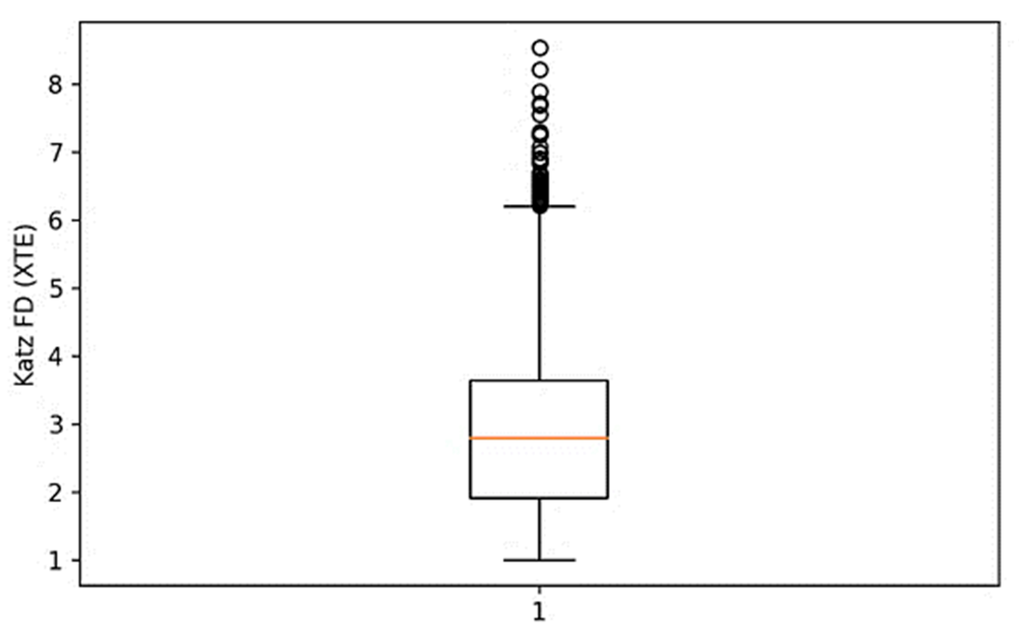
Figure 1 illustrates that, after coordinate and time normalization, the fractal metrics have consistent scales across different voyages.

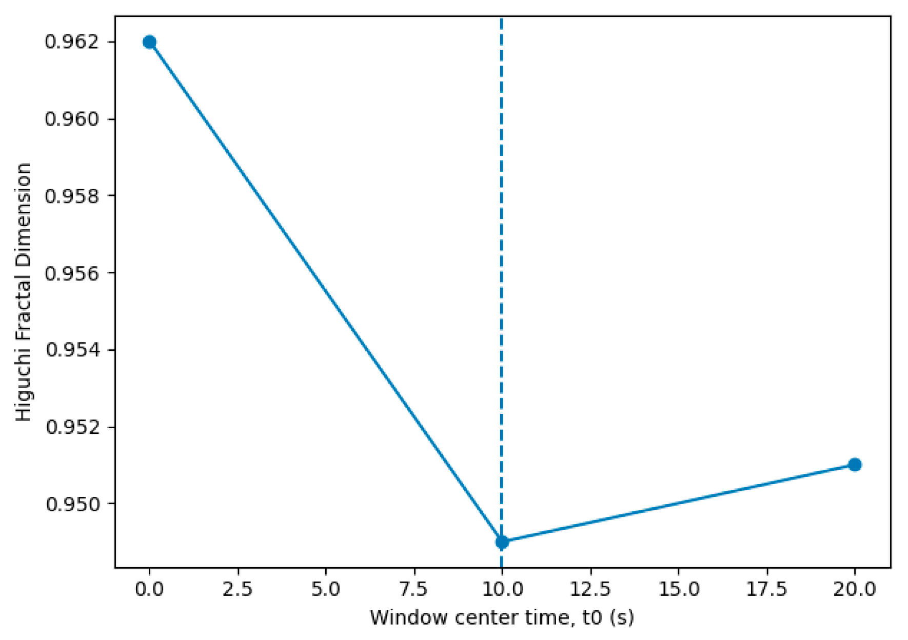
As shown in Figure 2, the Higuchi fractal dimension exhibits a pronounced local minimum, which reflects a temporary reduction in trajectory complexity and indicates a transition between maneuvering regimes. The parameter t₀ (window start in seconds) and the values of the Higuchi FD are computed in a unified metric system of time and space. It displays Higuchi_XTE^(j) over time with marking of windows where the value falls into the upper 5th percentile.

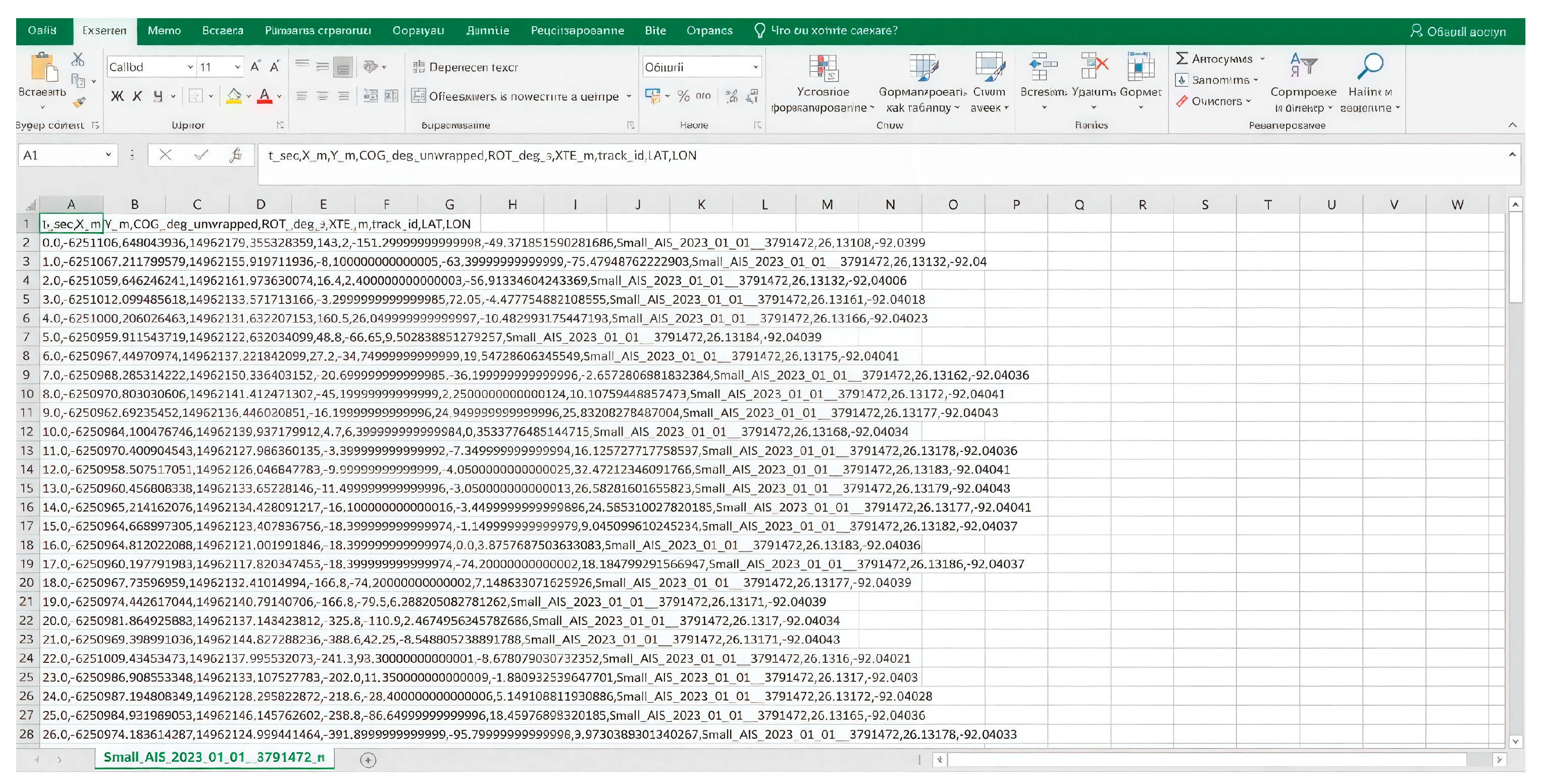
The structure of the file Export\fractal_report.csv as a summary of the normalization stage and primary fractal analysis is shown in Figure 3.

The table data can be used to demonstrate the structure S^(k). Thus, the developed automated reading and normalization procedure transforms heterogeneous AIS/ECDIS data into a unified, consistent metric trajectory model, providing a representation suitable for advanced analytical tasks based on fractal and nonlinear methods.

The next stage is the implementation of the second research task, which involves developing a system of fractal and dynamic indicators characterizing the geometry of vessel motion in sliding windows.

3.2. Software Implementation and Visualization Guidelines

All the described indicators are implemented within a single pipeline “AIS → Fractal conveyor + big data”. The key functions are:

-

higuchi_fd(ts), dfa_alpha(ts), katz_fd(ts), petrosian_fd(ts), box_count_fd(X, Y)—computation of fractal indicators;

-

sliding_metrics(ts, fs, WINDOW_SEC, STEP_SEC, metric_fn)—sliding window over the XTE signal;

-

step1_preprocess_ais()—formation of fractal_report.csv and fractal_windows.csv;

-

step2_fractal_signatures()—construction of the correlation matrix of fractal indicators and their clustering.

Based on the code execution results, illustrations are generated automatically (Figure 4):

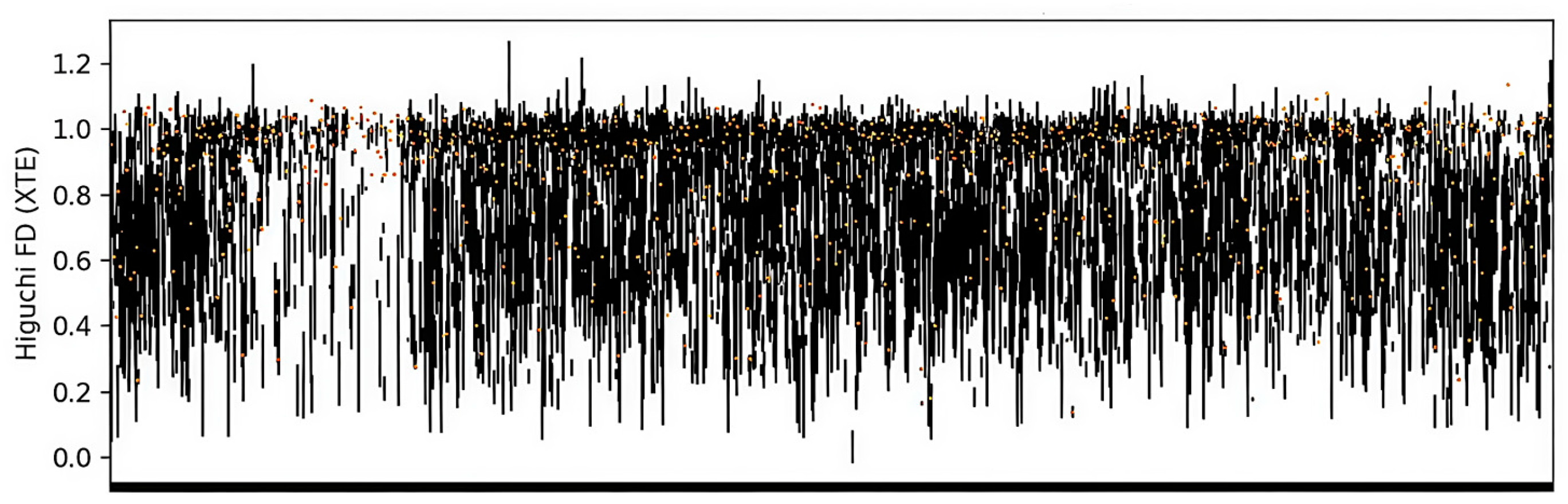
Each vertical segment in Figure 4 corresponds to a sliding analysis window positioned along the normalized vessel trajectory. The distribution illustrates the variability of local Higuchi FD(XTE) values across different tracks, while the width of the distribution reflects the degree of structural heterogeneity of cross-track deviations within individual voyages.

Elevated Higuchi FD values computed for the cross-track error (XTE) were seen as a signal that the geometric complexity of lateral motion with respect to the reference track had increased. In practical terms, such patterns can be correlated with the most intensive steering phases, such as docking operations, collision avoidance actions, route changes under environmental disturbances, or even navigation under strict traffic separation rules. The proposed fractal signature does not intend to directly classify the maneuver’s intent but rather offers a quantitative descriptor that can tell structured maneuvering behaviour apart from irregular or anomalous deviations.

Figure 5 shows boxplots of $\left\{D_{H,j}^{\mathrm{XTE}}\right\}$ for each vessel.

The correlation matrix in Figure 5 represents pairwise relationships between global fractal indicators computed for different motion components. Strong correlations indicate shared sensitivity to trajectory complexity, whereas weaker correlations reflect complementary aspects of vessel motion geometry captured by different fractal metrics.

As a practical illustrative example, Figure 4 and Figure 5 demonstrate a normalized vessel trajectory fragment together with the associated fractal indicators computed in sliding windows. This example shows how local geometric variations along the trajectory are reflected in the corresponding fractal metrics and can be interpreted in applied navigational analysis.

Together, the formal definitions and software implementation form a comprehensive system of fractal and dynamic indicators that provides a quantitative description of the geometric characteristics of a vessel’s motion both at the level of the entire trajectory and within the sliding window analysis. The proposed approach allows the formation of local fractal characteristics of motion while maintaining the temporal consistency and structural integrity of trajectory data, which is critically important for further analytical studies based on nonlinear methods.

Within the scope of the study, a unified fractal pipeline for processing ship trajectories based on AIS and ECDIS data was implemented and tested. The proposed approach was applied to navigation records characterized by uneven time discretization, gaps, and spatial inhomogeneities inherent in real operational data.

By applying time normalization and coordinate unification procedures, a metrically consistent representation of trajectories was obtained, ensuring the correct calculation of dynamic motion parameters, in particular, course, angular rate of turn, and transverse deviation. This enabled the elimination of distortions that arise during the direct analysis of raw AIS/ECDIS records.

The use of a sliding-window approach combined with fractal metrics enabled the formation of local fractal fields of the trajectory, reflecting changes in the complexity of the vessel’s movement over time. The results show that fractal indicators exhibit consistent behaviour across analysis windows and remain stable across different discretization parameters after data normalization.

A comparative analysis of global and local fractal characteristics showed that sliding-window analysis allows detection of structural heterogeneity in the trajectory, which is not apparent when averaging indicators over the entire route. This confirms the feasibility of using local fractal analysis to study the complex dynamics of ship movement.

Thus, the results obtained confirm the performance of the proposed fractal conveyor and its suitability for forming a stable, reproducible, and quantitative description of ship trajectories based on AIS/ECDIS data. In addition, the obtained results demonstrate that the proposed normalization and fractal processing pipeline produces consistent indicator values across trajectories with different sampling rates and spatial extents. This confirms that the framework ensures metric comparability of AIS/ECDIS-derived trajectories, which is a necessary prerequisite for subsequent comparative and structural analyses.

4. Discussion

The results confirm the feasibility of using a unified fractal conveyor to process ship trajectories based on AIS and ECDIS data. The proposed approach eliminates key limitations inherent in the analysis of raw navigation data, in particular, temporal heterogeneity, spatial inconsistency, and instability of derived dynamic parameters. This results in a metrically correct representation of the trajectory, suitable for the application of nonlinear analysis methods. At the same time, the applicability of the proposed framework is constrained by the characteristics of the source AIS and ECDIS data. In particular, downsampled AIS reporting intervals and sensor-level GNSS filtering may limit the sensitivity of fractal indicators to very short-term maneuvers. Therefore, the interpretation of local fractal metrics should be performed with consideration of data resolution and preprocessing effects.

The crucial point is that fractal indicators alone cannot serve as the basis for resolving the distinction between intentional moves and irregular acts. On the contrary, the suggested approach provides a structural delineation of motion dynamics that can be used for subsequent higher-level contextual or semantic analyses. Thus, fractal micromovement signatures serve as a diagnostic layer rather than a final classifier of navigational intent.

The proposed processing pipeline is inherently modular and paralleled execution from a computational standpoint. The steps of trajectory-level normalization and sliding-window fractal computations can be allocated to independent processing units in such a way that it will be efficient. The present study emphasizes the algorithmic formulation and methodological consistency; hence, runtimes and hardware specific optimizations are not included. Still, the framework can accommodate the large-scale batch processing of AIS datasets using the traditional systems of parallel computing. While remote sensing approaches such as synthetic aperture radar provide valuable capabilities for vessel detection and classification, they address a fundamentally different analytical level. The present work focuses on detailed trajectory dynamics derived from navigational records rather than object detection from imagery. Integration of trajectory-based fractal analysis with remote sensing outputs represents a complementary research direction but lies outside the scope of this study.

From an operational perspective, the developed framework is primarily suitable for onboard and post-voyage analytical tasks, including navigation performance assessment, trajectory reconstruction, and incident investigation. The approach is not intended for real-time VTS monitoring but provides a structured basis for detailed retrospective analysis of vessel motion dynamics using AIS and ECDIS records.

The maritime cybersecurity viewpoint considers the growing reliance on AIS and ECDIS data for analysis and making decisions as a factor that affects the data integrity, authenticity, and resilience. The AIS spoofing, GNSS interference, and unauthorized changes to the navigational data on board can directly impact the dependability of the trajectory indicators resulting from the analysis. Under these circumstances, the recommended processing framework might support retrospective integrity assessment by pointing out the irregular or unstructured motion patterns that could signal data tampering or cyber disturbances rather than normal navigational activities.

The use of a sliding-window approach in combination with a set of fractal indicators enables the study of local changes in the complexity of ship movement at different time scales. Unlike global trajectory characteristics, local fractal indicators allow the detection of structural heterogeneity of movement without losing the time reference. This is a significant advantage of the proposed approach over traditional statistical or kinematic methods, which typically average characteristics across the entire trajectory.

The primary objective of this study is methodological rather than benchmark-oriented validation. The proposed framework is designed to ensure structural comparability and internal consistency of trajectory-derived indicators, rather than to optimize numerical performance against a specific reference method. As such, the emphasis is placed on reproducibility, interpretability, and robustness of the processing pipeline. Quantitative benchmarking against alternative normalization schemes or window configurations represents a natural direction for future applied studies but is beyond the scope of the present work.

Particular attention should be paid to the robustness of fractal indicators to typical AIS/ECDIS data defects. The results show that after unified normalization and parametrically controlled segmentation with a sliding window, fractal indicators demonstrate stable behaviour even in the presence of noise and uneven discretization. This confirms the feasibility of using fractal analysis in combination with a clearly defined algorithmic pipeline.

5. Conclusions

The paper proposes a unified fractal conveyor for processing ship trajectories based on AIS and ECDIS data, converting raw, heterogeneous navigation records into a stable, reproducible metric model of movement. Unlike existing approaches that focus on individual preprocessing stages or the application of specific analytical indicators, the developed approach implements an end-to-end algorithmic scheme that combines time normalization, coordinate unification, dynamic parameter calculation, and sliding fractal analysis.

The proposed pipeline allows the formation of local fractal trajectory fields that characterize the complexity and structural features of ship movement at different time scales. The use of a set of fractal metrics, combined with a sliding-window approach, ensures the stability of the resulting indicators against noise, uneven sampling, and variations in input data, which are typical of AIS/ECDIS records.

The practical value of the proposed approach lies in its reproducibility, parametric transparency, and integration with maritime traffic analysis software systems. The developed fractal conveyor can serve as a universal basis for further analytical tasks related to trajectory dynamics, route comparison, and complex navigation processes.

References

1. Aloshan, M.A.; Sanad, E.M. An Integrated Framework for Architectural Visual Assessment: Validation of Visual Equilibrium Using Fractal Analysis and Subjective Perception. Buildings 2025, 16, 345. [Google Scholar] [CrossRef]
2. Alshanbari, H.M.; Bukhari, A.H.; Almazah, M.M.; Al-Rezami, A.Y. Multiscale Fractal Analysis for ADHD Disability Detection by EEG Signals: Integrating Grünwald–Letnikov Fractional Operators and Hurst Exponent Variability. Biomed. Signal Process. Control 2026, 114, 109332. [Google Scholar] [CrossRef]
3. Andronache, I.; Ciobotaru, A. Structural Change in Romanian Land Use and Land Cover (1990–2018): A Multi-Index Analysis Integrating Kolmogorov Complexity, Fractal Analysis, and GLCM Texture Measures. Geomatics 2025, 5, 78. [Google Scholar] [CrossRef]
4. Azzouz, A.; Bouhmidi, R.; Munir, M.E.; Nasralla, M.M.; Chetioui, M. Characterization and Analysis of Hybrid Fractal Antennas for Multiband Communication and Radar Applications. Fractal Fract. 2025, 10, 47. [Google Scholar] [CrossRef]
5. Hashemi Sababe, S.; Nikoufar, I. New Frontiers of Fractal Uncertainty. Fractal Fract. 2025, 9, 808. [Google Scholar] [CrossRef]
6. Bentahar, I.; Si Mhamdi, H.; Raji, M. Clustering Classification and Fractal Dimension Analysis of Structural Lineaments in the Amouguer–Michelifene Area (Central High Atlas, Morocco). J. Afr. Earth Sci. 2025, 233, 105865. [Google Scholar] [CrossRef]
7. Dai, Q.; Liu, X.; Ma, X.; Tian, S.; Cui, Q. Research Status and Prospects of the Fractal Analysis of Metal Material Surfaces and Interfaces. Int. J. Miner. Metall. Mater. 2025, 32, 20–38. [Google Scholar] [CrossRef]
8. Dobrescu, G.; Papa, F.; State, R. Fractal Analysis and Fractal Dimension in Materials Chemistry. Fractal Fract. 2024, 8, 583. [Google Scholar] [CrossRef]
9. Estévez-Sánchez, K.H.; Del Rosario-Santiago, J.; Cortés-Zavaleta, O.; Sánchez-Cantú, M.; Ruiz-Espinosa, H.; García-Alvarado, M.A.; Ochoa-Velasco, C.E.; Ruiz-López, I.I. A Comparative Study of 3D CAD and Fractal Geometry Models for Analyzing Mass Transfer in Shrimp during Convective Drying. Food Bioprod. Process. 2025, 154, 532–541. [Google Scholar] [CrossRef]
10. Guo, L.; Xin, X.; He, K. Study on Permeability Coefficient of Saturated Clay Modified by Fractal Theory and Poiseuille Theory. Materials 2025, 19, 21. [Google Scholar] [CrossRef]
11. Liu, X.; Fu, X.; Song, D.; Zhang, Y.; Liu, R. Acid-Induced Pore Evolution in Coal: Multiscale Fractal Analysis and Implications for Gas Transport Dynamics. Results Eng. 2025, 27, 106999. [Google Scholar] [CrossRef]
12. Meng, F.; Zhang, Q.; Wu, T.; Song, E.; Li, Y.; Sun, Y.; Liu, X. Fractal Characteristics and Pore Structures of Shales from the Doushantuo Formation, Yichang Area, South China. Fractal Fract. 2025, 9, 774. [Google Scholar] [CrossRef]
13. Peng, Y.; Zhang, X.; Chen, X. Impact of Fractal Dimension on Recycled Aggregate Concrete Performance. J. Mater. Res. Technol. 2025, 39, 3007–3020. [Google Scholar] [CrossRef]
14. Pan, T.; Xu, X.; Zheng, Y.; Wu, L.; Yang, C.; Aydin, B.B.; Li, Y.; Zhou, Y. Acoustic Emission-Driven Fractal Analysis for Damage Warning in FRP-Strengthened Corroded RC Beams. Eng. Fract. Mech. 2025, 328, 111563. [Google Scholar] [CrossRef]
15. Song, Y.; Dong, W.; Xue, G.; Lin, Y. Capillary Water Absorption Characteristics of Aeolian Sand Concrete. Constr. Build. Mater. 2025, 492, 142994. [Google Scholar] [CrossRef]
16. Stanchev, P.; Hinov, N. Composite Fractal Index for Assessing Voltage Resilience in RES-Dominated Smart Distribution Networks. Fractal Fract. 2025, 10, 32. [Google Scholar] [CrossRef]
17. Swaidan, B.; Paul, I.; Yu, S.C.M. Hierarchical Fractal Surface Patterns for Enhanced Gypsum Scaling Resistance. J. Water Process Eng. 2025, 78, 108700. [Google Scholar] [CrossRef]
18. Wang, J.; Zhou, H.; Lu, M.; Zhang, L.; Wang, Z.; Li, H.; Mao, T.; Shi, F.; Xue, D. Fractal Analysis of Pore–Fracture Evolution in Deep Coal under Temperature Effect. Fuel 2026, 408, 137534. [Google Scholar] [CrossRef]
19. Wang, M.; Yu, X.; Liu, S.; Cheng, Y.; Guo, J.; Wang, Z.; Duan, X. Sedimentary Paleo-Environment and Reservoir Heterogeneity Revealed by Fractal Analysis. Fractal Fract. 2025, 9, 795. [Google Scholar] [CrossRef]
20. Xu, M.; Guo, Y.; Mao, H.; Li, Y.; Shi, X.; Ma, H.; He, Y.; Fang, J. Mechanical Damage and Permeability Evolution of Tight Sandstone. Processes 2025, 13, 3919. [Google Scholar] [CrossRef]
21. Xu, Q.; Xia, Z.; Du, S.; Fan, Y.; Huang, G.; Chen, S.; Zhang, Z.; Liu, Y. Fractal and CT Analysis of Water-Bearing Coal–Rock Composites. Fractal Fract. 2025, 9, 782. [Google Scholar] [CrossRef]
22. Benocci, R.; Guagliumi, G.; Potenza, A.; Zaffaroni-Caorsi, V.; Roman, H.E.; Zambon, G. Wavelet-Based Analysis of Soundscape Dynamics in a Riparian Woodland: The Bernate-Ticino River Park. Sensors 2025, 25, 7248. [Google Scholar] [CrossRef] [PubMed]
23. Esteban, F.J.; Vargas, E. Foundations and Clinical Applications of Fractal Dimension in Neuroscience: Concepts and Perspectives. AppliedMath 2025, 6, 7. [Google Scholar] [CrossRef]
24. Hashimov, E.; Pashayev, A.; Khaligov, G. Camera Control Algorithm and Image Quality Assessment Method to Obtain a Quality Image. Adv. Inf. Syst. 2025, 9, 50–56. [Google Scholar] [CrossRef]
25. Hurin, A.; Khudov, H.; Kostyria, O.; Maslenko, O.; Siadrystyi, S. Comparative Analysis of Spectral Anomalies Detection Methods on Images from On-Board Remote Sensing Systems. Adv. Inf. Syst. 2024, 8, 48–57. [Google Scholar] [CrossRef]
26. Iványi, D.; Kivovics, M.; Balázs, R.; Németh, O. Fractal Analysis as a Predictor of Early Implant Loss: A Retrospective Study. Int. Dent. J. 2025, 75, 103880. [Google Scholar] [CrossRef]
27. Khudov, H.; Makoveichuk, O.; Kalimulin, T.; Khudov, V.; Shamrai, N. Approximating the Edge Detection Convolutional Operator Using a Genetic Algorithm for Segmentation of Complex-Structured Images. Adv. Inf. Syst. 2024, 8, 5–12. [Google Scholar] [CrossRef]
28. Maatki, C.; Murtaza, S.; Khan, M.N.; Alrasheedi, N.H.; Alshammari, B.M.; Kolsi, L. Mesh-Free Modeling and Analysis of Fractal–Fractional Thermoelectric Fluid Flow Model with Thermal Radiation in Microchannel Systems. J. Radiat. Res. Appl. Sci. 2025, 18, 101984. [Google Scholar] [CrossRef]
29. Tyagi, A.; Vashistha, S. Fractal Generation via Khan Iteration. Chaos Solitons Fractals 2025, 201, 117184. [Google Scholar] [CrossRef]
30. Valjarevic, S.; Paunovic Pantic, J.; Cumic, J.; Corridon, P.R.; Pantic, I. Fractal Analysis of Auditory Evoked Potentials: Research Gaps and Potential AI Applications. Fractal Fract. 2025, 10, 20. [Google Scholar] [CrossRef]
31. Vujović, I.; Šoda, J.; Golub Medvešek, I. Review of Trends in Wavelets with Possible Maritime Applications. Signals 2025, 6, 70. [Google Scholar] [CrossRef]
32. Tadić, L.; Golub Medvešek, I.; Vujović, I.; Šoda, J. Infrared Thermography in Maritime Systems: A Systematic Review. Appl. Sci. 2025, 15, 12551. [Google Scholar] [CrossRef]
33. Enguehard, R.A.; Ware, C. Interactive Exploration of Movement Data: A Case Study of Geovisual Analytics for Fishing Vessel Analysis. Inf. Vis. 2013, 12, 234–245. [Google Scholar] [CrossRef]
34. Hu, Q.; Wu, Z.; Wu, Y.; Guo, Z. Risk Prediction of Marine Traffic Based on Fractal Interpolation Algorithm. In Proceedings of the IEEE International Conference on Industrial Engineering and Engineering Management, Hong Kong, China, 8–11 December 2009; pp. 2504–2508. [Google Scholar] [CrossRef]
35. Kobets, V.; Popovych, I.; Zinchenko, S.; Nosov, P.; Tovstokoryi, O.; Kyrychenko, K. Control of the Pivot Point Position of a Conventional Single-Screw Vessel. In Proceedings of the ICST 2023, Odesa, Ukraine, 21–23 September 2023; Odessa National Polytechnic University: Odessa, Ukraine, 2023; Volume 3513, pp. 130–140. [Google Scholar]
36. Li, J.; Liu, H.; Chen, X.; Li, J.; Xiang, J. Vessel Pattern Recognition Using Trajectory Shape Feature. In Proceedings of the CSAI 2021; ACM: New York, NY, USA, 2021. [Google Scholar] [CrossRef]
37. Pfoser, D.; Jensen, C.S.; Theodoridis, Y. Novel Approaches to the Indexing of Moving Object Trajectories. In Proceedings of the VLDB 2000, Cairo, Egypt, 10–14 September 2000; pp. 395–406. [Google Scholar]
38. Wang, J.; Zhou, Y.; Cao, X.; Wang, Y.; Zhu, C.; Zhang, W. Shape-Based Analysis for Vessel Trajectories. In Proceedings of the ACM SIGSPATIAL 2017; ACM: New York, NY, USA, 2017. [Google Scholar] [CrossRef]
39. Turna, İ.; Öztürk, O.B. A Causative Analysis on ECDIS-Related Grounding Accidents. Ships Offshore Struct. 2020, 15, 792–803. [Google Scholar] [CrossRef]
40. Nosov, P.; Melnyk, O.; Malaksiano, M.; Mamenko, P.; Onyshko, D.; Fomin, O.; Píštěk, V.; Kučera, P. Machine Learning-Based Semantic Analysis of Scientific Publications for Knowledge Extraction in Safety-Critical Domains. Mach. Learn. Knowl. Extr. 2025, 7, 150. [Google Scholar] [CrossRef]
41. Romanuke, V.V.; Romanov, A.Y.; Malaksiano, M.O. Genetic Algorithm Improvement by Tour Constraint Violation Penalty Discount for Maritime Cargo Delivery. Syst. Res. Inf. Technol. 2023, 2, 104–126. [Google Scholar] [CrossRef]
42. Theodoridis, Y.; Silva, J.R.O.; Nascimento, M.A. On the Generation of Spatiotemporal Datasets. In Lecture Notes in Computer Science; Springer: Berlin, Germany, 1999; Volume 1651, pp. 131–147. [Google Scholar]
43. Uthayakumar, P.; Tharani, S.; Agathiyan, A.; Akgül, A. Fractal Dimension Analysis of Stock Indices. J. Comput. Appl. Math. 2026, 474, 117008. [Google Scholar] [CrossRef]
44. Volkov, V.; Gritsuk, I.; Volkova, T.; Berezhnaja, N.; Pliekhova, G.; Bulgakov, M.; Marmut, I.; Volska, O. System Approach to Forecasting Standards of Vehicles’ Braking Efficiency; SAE Technical Paper 2021-01-5083; SAE International: Warrendale PA, USA, 2021. [Google Scholar] [CrossRef]
45. Wang, L.; Qin, Z.; Zhang, Z.; Zhang, J. Free Metaplectic K-Wigner Distribution. Fractal Fract. 2025, 9, 245. [Google Scholar] [CrossRef]
46. Wang, X.; Guo, S. Dynamic Analysis of a Family of Iterative Methods with Fifth-Order Convergence. Fractal Fract. 2025, 9, 783. [Google Scholar] [CrossRef]
47. Wang, Z.; Chen, Y.; Zheng, M. Fractal Dimension Analysis of Spatial Distribution Rationality of Urban Fire Stations. J. Urban Manag. 2025, in press. [Google Scholar] [CrossRef]
48. Widodo, W.; Ernowo, E.; Pratama, R.N.; Noor, M.R.; Widhiyatna, D.; Putra, E.; Idrus, A.; Pardiarto, B.; Boakes, Z.; Parningotan, M.R.; et al. Integrating PCA and Fractal Modeling for Identifying Geochemical Anomalies. Geosciences 2025, 15, 470. [Google Scholar] [CrossRef]
49. Ren, G.; Wan, L. Sustainable Cold Region Urban Expansion Assessment through Impervious Surface Classification and GDP Spatial Simulation. Sustainability 2024, 17, 11363. [Google Scholar] [CrossRef]
50. Zinchenko, S.; Kyrychenko, K.; Grosheva, O.; Nosov, P.; Popovych, I.; Mamenko, P. Automatic Reset of Kinetic Energy in Case of Inevitable Collision of Ships. In Proceedings of the ACIT 2023; IEEE: New York, NY, USA, 2023; pp. 496–500. [Google Scholar] [CrossRef]
51. Bilohub, A.; van Duong, N.; Sirenko, F.; Savchuk, V.; Bilousov, I.; Symonenko, R.; Zajačko, I. Analysis of Heat Transfer Coefficients for Simulation of the Heat Exchange between Oil and the Internal Cavity Faces of the Isolated Piston at Variable Gravity Conditions. IOP Conf. Ser. Mater. Sci. Eng. 2020, 776, 012020. [Google Scholar] [CrossRef]
52. Fomin, O.; Gorbunov, M.; Lovska, A.; Gerlici, J.; Kravchenko, K. Dynamics and Strength of Circular Tube Open Wagons with Aluminum Foam Filled Center Sills. Materials 2021, 14, 1915. [Google Scholar] [CrossRef]
53. Koskina, Y.; Onyshenko, S.; Drozhzhyn, O.; Melnyk, O. Efficiency of Tramp Fleet Operating under the Contracts of Affreightment. Sci. J. Silesian Univ. Technol. Ser. Transp. 2023, 120, 137–149. [Google Scholar] [CrossRef]
54. Melnyk, O.M.; Onishchenko, O.A.; Shyshkin, O.V.; Volkov, O.M.; Volyanskyy, S.M.; Maulevych, V.O.; Kreitser, K.O. Enhancing Shipboard Technical Facility Performance through the Utilization of Low-Sulfur Marine Fuel Grades. J. Chem. Technol. 2024, 32, 233–245. [Google Scholar] [CrossRef]
55. Melnyk, O.; Onyshchenko, S.; Onishchenko, O.; Koskina, Y.; Lohinov, O.; Veretennik, O.; Stukalenko, O. Fundamental Concepts of Deck Cargo Handling and Transportation Safety. Eur. Transp.—Trasp. Eur. 2024, 98, 1. [Google Scholar] [CrossRef]
56. Onishchenko, O.; Bukaros, A.; Melnyk, O.; Yarovenko, V.; Voloshyn, A.; Lohinov, O. Ship Refrigeration System Operating Cycle Efficiency Assessment and Identification of Ways to Reduce Energy Consumption of Maritime Transport. In Studies in Systems, Decision and Control; Springer: Cham, Switzerland, 2023; Volume 481, pp. 641–652. [Google Scholar] [CrossRef]
57. Sulym, A.O.; Fomin, O.V.; Khozia, P.O.; Mastepan, A.G. Determination of Parameters of On-Board Capacitive Energy Storage of Rolling Stock. Nauk. Visnyk NHU 2018, 5, 79–87. [Google Scholar] [CrossRef]
58. Varbanets, R.; Minchev, D.; Savelieva, I.; Rodionov, A.; Mazur, T.; Psariuk, S.; Bondarenko, V. Advanced Marine Diesel Engines Diagnostics for IMO Decarbonization Compliance. AIP Conf. Proc. 2024, 3104, 020004. [Google Scholar] [CrossRef]
59. Varbanets, R.; Minchev, D.; Kucherenko, Y.; Zalozh, V.; Kyrylash, O.; Tarasenko, T. Methods of Real-Time Parametric Diagnostics for Marine Diesel Engines. Pol. Marit. Res. 2024, 31, 71–84. [Google Scholar] [CrossRef]
Figure 1. Distribution of Katz FD for XTE across all trajectories.
Digital 06 00011 g001
Figure 2. Evolution of the Higuchi fractal dimension computed for the normalized vessel trajectory in sliding windows.
Digital 06 00011 g002
Figure 3. Tabular data for a fragment of the normalized vessel trajectory.
Digital 06 00011 g003
Figure 4. Distribution of sliding Higuchi FD(XTE) values over tracks.
Digital 06 00011 g004
Figure 5. Correlation matrix illustrating pairwise relationships between fractal indicators computed for different components of vessel motion after trajectory normalization.
Digital 06 00011 g005
Disclaimer/Publisher’s Note: The statements, opinions and data contained in all publications are solely those of the individual author(s) and contributor(s) and not of MDPI and/or the editor(s). MDPI and/or the editor(s) disclaim responsibility for any injury to people or property resulting from any ideas, methods, instructions or products referred to in the content.