Simple Summary
This study aimed to evaluate the characteristics of short acquisition times using the Clear adaptive Low-noise Method and Advanced intelligent Clear-IQ Engine (AiCE) reconstructions in a semiconductor-based positron emission tomography/computed tomography system. While a significant reduction in the acquisition time was not achievable with three-dimensional ordinary Poisson ordered-subset expectation maximization (OSEM) with time-of-flight reconstruction alone, the addition of point spread function correction suggested potential for a further reduction in acquisition time. Although AiCE reconstruction did not achieve all the recommended values simultaneously, no substantial discrepancy was observed between the calculated values and recommended thresholds.
Abstract
This study aimed to evaluate the characteristics of short acquisition times using the Clear adaptive Low-noise Method (CaLM) and Advanced intelligent clear-IQ engine (AiCE) reconstructions in a semiconductor-based positron emission tomography (PET)/computed tomography system. PET data were acquired for 30 min in list mode and resampled into time frames ranging from 15 to 120 s. Images were reconstructed using three-dimensional ordinary Poisson ordered-subset expectation maximization (OSEM) with time of flight (TOF) and OSEM with TOF and point spread function modeling (PSF) algorithms, with OSEM iterations adjusted from 1 to 20 and CaLM applied under Mild, Standard, and Strong settings. AiCE reconstruction allows for the modification of only the acquisition time. The images were evaluated based on the coefficient of variation, recovery coefficient, % background variability (N10mm), % contrast-to-% background variability ratio (QH10mm/N10mm), and contrast-to-noise ratio. While OSEM with TOF reconstruction did not significantly reduce the acquisition time, the addition of PSF correction suggested the potential for further reduction. Given that the AiCE characteristics may vary depending on the equipment used, further investigation is required.
1. Introduction
18F-fluorodeoxyglucose (FDG) positron emission tomography/computed tomography (PET/CT) is commonly used for benign–malignant tumor differentiation, cancer staging, primary tumor definition, therapy prediction, and radiation therapy planning [1,2]. However, 18F-FDG PET/CT has the disadvantage of low resolution, which is compensated for by extending the imaging time or increasing the dose of the radiopharmaceutical. In particular, PET/CT images often contain significant amounts of noise. Therefore, post-smoothing methods such as Gaussian filtering are commonly employed for short acquisition times and standard examinations. However, these methods can cause a deterioration in spatial resolution and lead to the underestimation of semi-quantitative measurements [3,4].
The Cartesion Prime (Canon Medical Systems, Tokyo, Japan) used in this study is equipped with a filter called Clear adaptive Low-noise Method (CaLM), which is based on the Non-Local Means (NLM) method [5]. The NLM filter, proposed by Buades et al., effectively reduces noise while preserving spatial resolution [6]. The weighting factor used in the Non-Local Means filter was calculated (Formula (1)):
where h is the smoothing parameter, which is empirically determined by the user. xi is the pixel of interest, and xj is the central pixel of the template layer. The similarity between the two is calculated from the L2 norm convolved with a Gaussian kernel with a standard deviation of a. Z(i) is the normalization factor, calculated using (Formula (2)):
The Gaussian filter that has been used so far applies weights to the entire image and has excellent noise reduction effects (Figure 1a). However, it also causes a reduction in the signal (Figure 1b). In contrast, the NLM filter reduces only the noise in the image while preserving the signal [6]. Due to this advantage, attempts to apply NLM to PET images have been made, and its effectiveness has been demonstrated [4]. The only drawback of NLM is that the parameter h is set by the user, meaning that the filter strength applied to the image may vary depending on the user [7,8]. The CaLM of Cartesian Prime has three parameters related to noise smoothing in the image, Mild, Standard, and Strong, which are relatively simple. However, it is important to understand what kind of smoothing effect these parameters produce. Since the actual calculation formula used by CaLM is a black box, it is difficult to independently investigate the detailed smoothing effect. Therefore, in this study, the noise reduction effect of CaLM was investigated from the perspective of physical indicators.
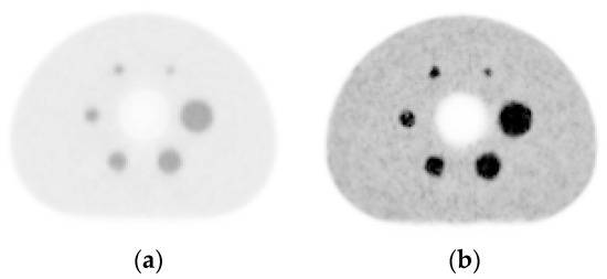
Figure 1.
(a) The image with a Gaussian filter applied, (b) the image with CaLM applied.
Recently, the development of semiconductor-based PET/CT systems has become widespread. These systems can detect more photon events with the same dose and scan time as conventional systems, leading to improved image quality compared with traditional PET/CT systems [9,10]. Consequently, numerous studies have suggested that small lesions can be detected even with short acquisition times [11,12]. However, these reports focused on the detection of small lesions and did not rely on quantitative evaluations based on guidelines. Furthermore, the reported studies primarily focused on shortening the acquisition time, with no changes made to the image reconstruction parameters [13,14,15]. In fact, in the study by Pedro et al., not only the acquisition time but also the image reconstruction parameters were varied when acquiring phantom images, clearly demonstrating the capabilities of PET/CT [16]. Since PET image quality varies depending on the image reconstruction parameter set, it is necessary to optimize the reconstruction parameters for short acquisition times, as well. To provide better images, evaluating the detection capability of small lesions is necessary, as well as optimizing the image reconstruction parameters and performing quantitative evaluations using the physical indicators specified in guidelines. Alqahtani et al. concluded that short acquisition times are necessary to reduce patient examination burden, but they also increase the amount of noise in the image and thus require the optimization of image reconstruction parameters [17]. Zhao et al. concluded that the optimization of image reconstruction parameters is essential to achieve high-quality images and quantitative accuracy [18]. Therefore, the effects of image reconstruction parameters not only on conventional PET/CT systems but also on semiconductor-based PET/CT systems must be investigated to achieve short acquisition times.
Cartesion Prime is also equipped with an AI technology known as the Advanced intelligent Clear-IQ Engine (AiCE) [19], which has been widely reported to enhance image quality and improve visualization capabilities [10,20,21]. This technology is a noise reduction process reported by Tsuchiya et al. [22]., which applies the residual network (ResNet). The AiCE network consists of an 8-layer deep convolutional neural network (DCNN) and performs residual learning using long-acquisition-time images as training data [19]. Rather than estimating high-quality images, this technology estimates the noise and outputs the image. Due to this feature, it is possible that noise generated during short acquisition times can be effectively removed by estimating the noise. However, the reports to date have primarily focused on investigating depiction capabilities, with no mention of performance evaluation. Therefore, AiCE should be applied to clinical images with a thorough understanding of its characteristics.
For these reasons, the use of CALM and AiCE reconstructions could provide high-quality images capable of depicting small lesions, even over short acquisition times.
This study aimed to evaluate the characteristics of short acquisition times using CaLM and AiCE reconstructions implemented in a semiconductor-based PET/CT system.
2. Materials and Methods
2.1. Data Acquisition
The PET/CT system used in this study was the Cartesion Prime. The specifications of this system are listed in Table 1. The CT imaging conditions were as follows: tube voltage, 120 kV; tube current, volume exposure control; collimation, 0.5 mm × 80; scan speed, 0.5 s; and slice thickness, 2 mm. The experiments were performed according to the “Japanese Guideline for Oncology FDG PET/CT Data Acquisition Protocol: synopsis of Version 2.0” [1]. We used a body phantom from the National Electrical Manufacturers Association (NEMA) and International Electrotechnical Commission. The hot spheres and background of the NEMA body phantom were filled with an 18F-FDG solution at a radioactivity ratio of 4:1. PET data were acquired for 30 min in list mode and resampled into time frames from 15 to 120 s in 15 s increments to simulate different acquisition times.

Table 1.
Specifications of the PET/CT system.
2.2. Image Reconstruction
The acquired PET data were reconstructed using three-dimensional ordinary Poisson ordered-subset expectation maximization (OSEM) with time of flight (TOF), with or without point spread function (PSF) modeling, resulting in two different combinations of reconstruction algorithms: OSEM with TOF and OSEM with TOF and PSF. The number of iterations for OSEM reconstruction was sequentially varied from 1 to 20 for images at each acquisition time, with the subset number fixed at 12. In addition, the intensity of CaLM applied to the reconstructed images was adjusted to be Mild, Standard, or Strong. In AiCE reconstruction, parameters such as the number of iterations and subsets cannot be applied. Therefore, it was applied only to eight types of images obtained with acquisition times ranging from 15 to 120 s in 15 s increments.
2.3. Analyses of Phantom Images
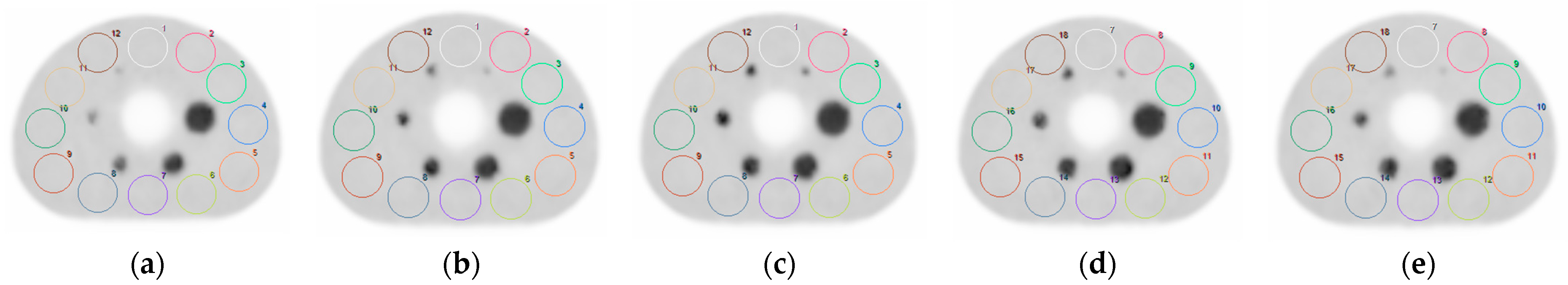
According to the “Japanese guideline for the oncology FDG-PET/CT data acquisition protocol: Synopsis of Version 2.0” [1], twelve circular regions of interest (ROIs) were placed at ±1 cm and ±2 cm from the slice where each sphere (Figure 2), ranging from 10 mm to 37 mm in diameter, was most clearly visualized, in order to calculate the coefficient of variation (CV), recovery coefficient (RC), %background variability (N10mm), and %contrast-to-N10mm (Q10mm/N10mm). Twelve circular 37 mm ROI spheres were set in the BG, where a slice contained clear representations of all sizes of spheres to determine the CV. The counts in each ROI were calculated as CV (Formula (3)):
where CB,37mm and SD37mm are the respective mean count and standard deviation in each 37 mm ROI sphere in the BG. The RC of each sphere was calculated by placing an ROI in the slice with hot spheres as follows (Formula (4)):
where Cj is the maximum total value obtained from each hot sphere j, and C37mm is the average of the maximum pixel values obtained from the 37 mm sphere across all slices. However, because the guidelines only define the resolution for 10 mm spheres, RC10mm was calculated for 10 mm spheres in this study. N10mm was calculated using the average CV of the 10 mm ROIs placed on each slice, as follows (Formula (5)):
where CB,10mm and SD10mm represent the average count and standard deviation in the ROI with a diameter of 10 mm in the BG, respectively. SD10mm was calculated as follows (Formula (6)):
where k is 10 mm, and K is 60 (12 ROIs on five slices, 60 in total). The contrast-to-noise ratio (CNR) was used to demonstrate object detectability based on the Rose criterion (CNR > 5) [23]. The CNR was calculated as follows (Formula (7)):
where CH,average,j represents the average number of counts in each sphere j, CB,average,j represents the average number of counts in the background volume j, and SDB,average,j represents the average standard deviation of background volume j.
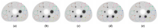
Figure 2.
The slice on which the hot spheres were most clearly visualized was defined as the center slice. ROIs were placed on the center slice, as well as on the slices located at ±1 cm and ±2 cm from it. (a–e) The −2 cm, −1 cm, center, +1 cm, and +2 cm slices.
The ROI data were analyzed using the VirtualPlace ver.3.8 software (AZE, Inc., Tokyo, Japan).
2.4. Analysis of Phantom Images
Based on the work of Yamagiwa et al., the image quality of AiCE reconstruction was evaluated using a 5-point scale based on the following quality criteria: 10 mm sphere visualization, ranging from 1 (not discernible) to 5 (excellent visualization); overall image quality, ranging from 1 (poor overall quality) to 5 (excellent overall quality); and image noise, ranging from 1 (severely interfering noise) to 5 (no perceivable relevant noise) [10].
These visual assessments were performed by three radiological technologists, each with more than 5 years of experience in nuclear medicine.
3. Results
3.1. Image Analysis Using OSEM Reconstruction
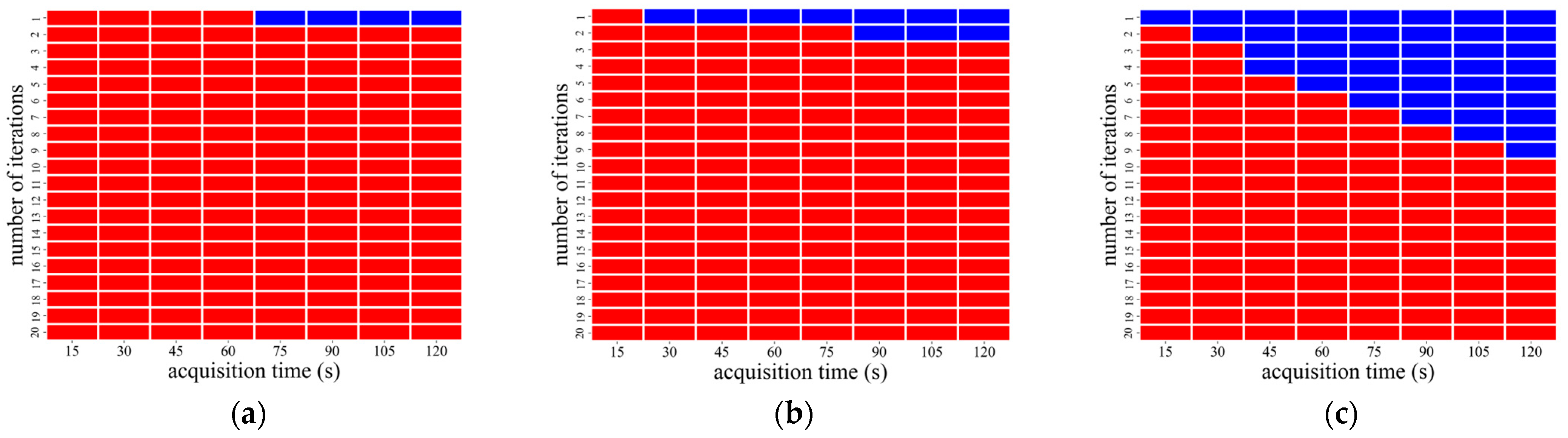
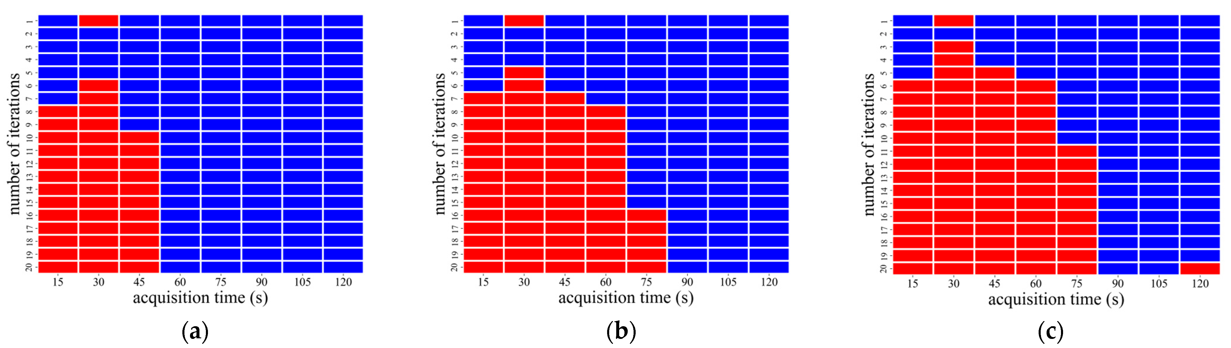
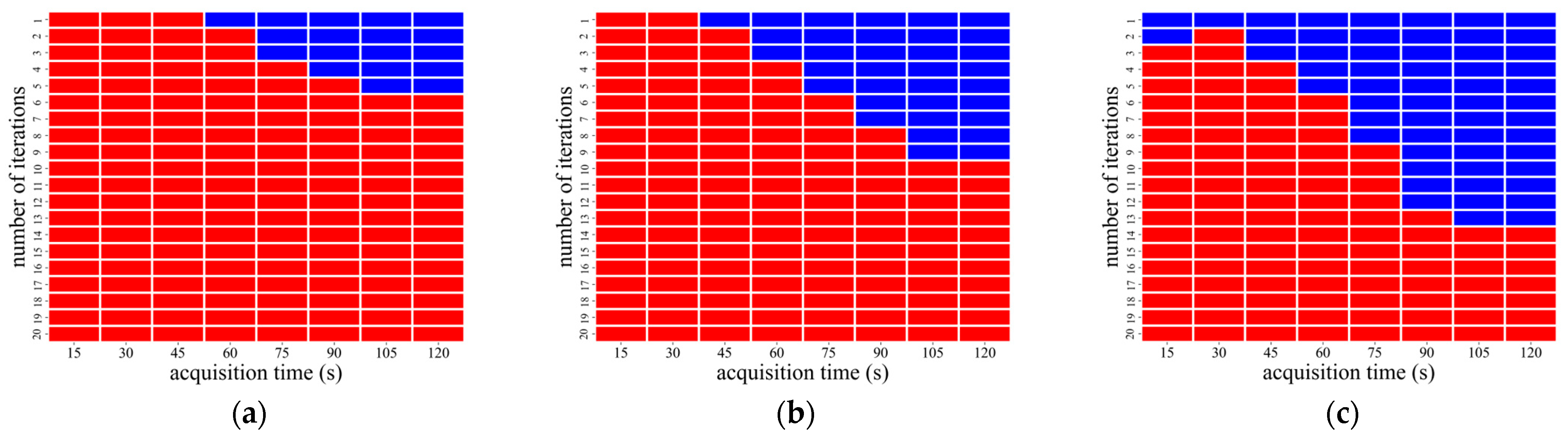
Figure 3 shows the CV results reconstructed using OSEM with TOF, and Figure 4 shows those reconstructed using OSEM with TOF and PSF. For OSEM with TOF reconstruction, the CV exhibited similar trends among the Mild, Standard, and Strong CaLM settings. As the intensity of CaLM increased from Mild to Standard and Strong, more image reconstruction parameters were required to achieve the recommended values. A similar trend was observed for OSEM with TOF and PSF reconstruction. Compared to OSEM with TOF reconstruction, OSEM with TOF and PSF reconstruction achieved the recommended values for more image reconstruction parameters. In both OSEM with TOF and OSEM with TOF and PSF reconstruction, the recommended values were achieved as the acquisition time increased.
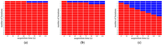
Figure 3.
Coefficient of variation (CV) results for three-dimensional ordinary Poisson ordered-subset expectation maximization with time-of-flight (OSEM with TOF) reconstruction. (a–c) Mild, Standard, and Strong clear adaptive low-noise method (CaLM) settings. In the figure, red indicates image reconstruction conditions that did not meet the guideline’s recommended criteria, while blue indicates those that did (CV < 10%).

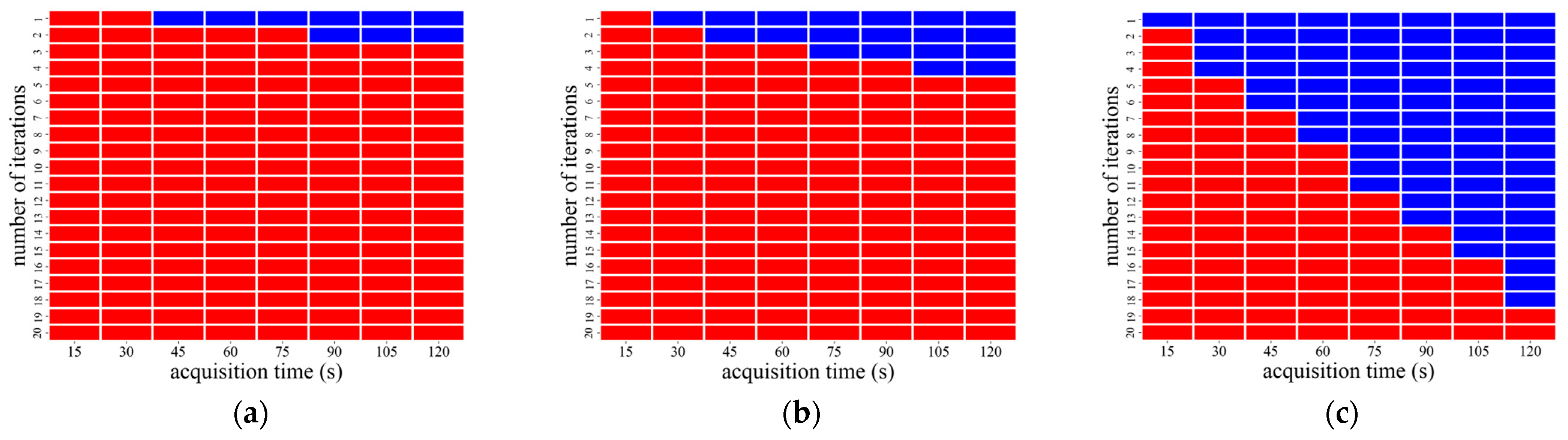
Figure 4.
CV results from the OSEM with TOF and point spread function (PSF) reconstruction. (a–c) Mild, Standard, and Strong CaLM settings. In the figure, red indicates image reconstruction conditions that did not meet the guideline’s recommended criteria, while blue indicates those that did (CV < 10%).
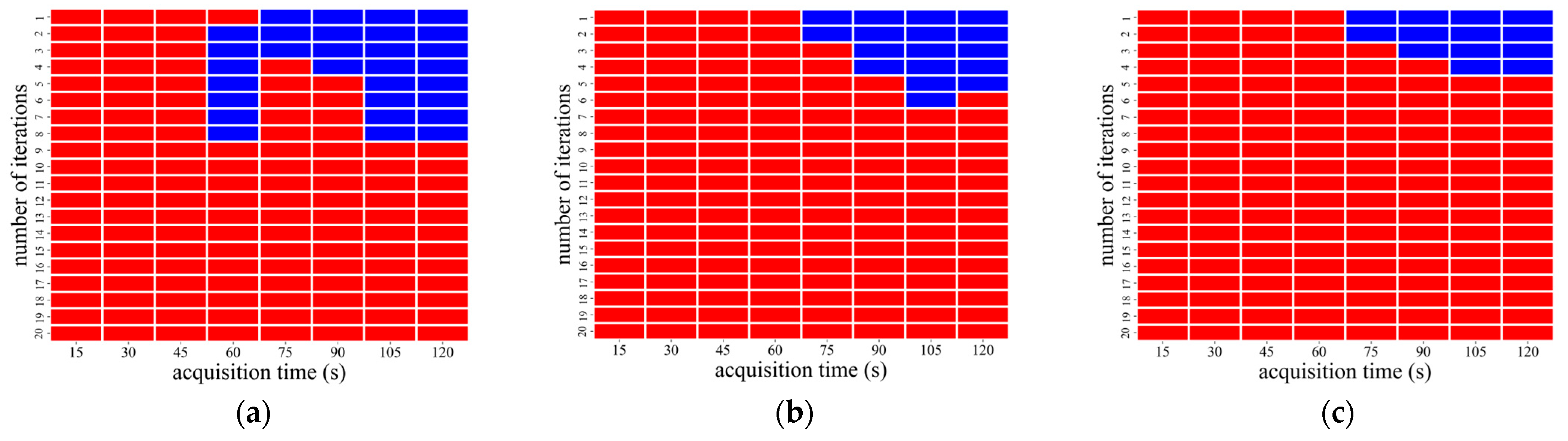
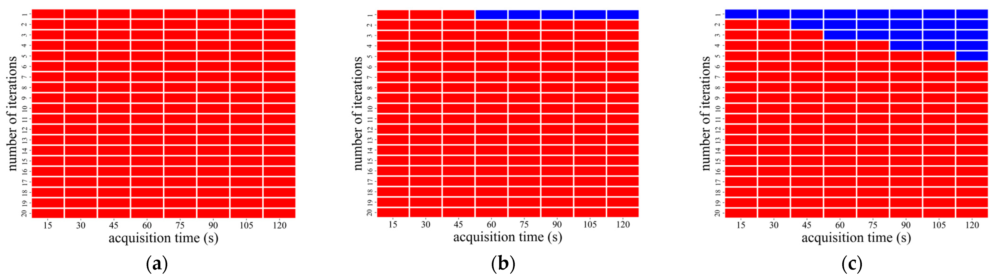
Figure 5 shows the RC results reconstructed using OSEM with TOF, and Figure 6 shows those reconstructed using OSEM with TOF and PSF. For the OSEM with TOF reconstruction, RC exhibited similar trends among the Mild, Standard, and Strong CaLM settings. As the intensity of CaLM increased from Mild to Standard and Strong, RC10mm tended to decrease. At the same acquisition time, RC was more likely to achieve the recommended values when the CaLM intensity was lower. Similar trends were observed for the OSEM with TOF and PSF reconstruction. Compared with OSEM with TOF, OSEM with TOF and PSF reconstruction achieved the recommended values under more image reconstruction conditions. In both OSEM with TOF and OSEM with TOF and PSF reconstruction, the recommended values were achieved as the acquisition time increased.
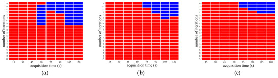
Figure 5.
Recovery coefficient results calculated for 10 mm spheres (RC10mm) from OSEM with TOF reconstruction. (a–c) Mild, Standard, and Strong CaLM settings. In the figure, red indicates image reconstruction conditions that did not meet the guideline’s recommended criteria, while blue indicates those that did (RC ≥ 38%).
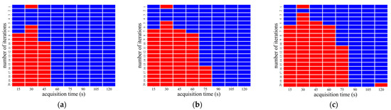
Figure 6.
RC10mm results from OSEM with TOF and PSF reconstruction. (a–c) Mild, Standard, and Strong CaLM settings. In the figure, red indicates image reconstruction conditions that did not meet the guideline’s recommended criteria, while blue indicates those that did (RC ≥ 38%).
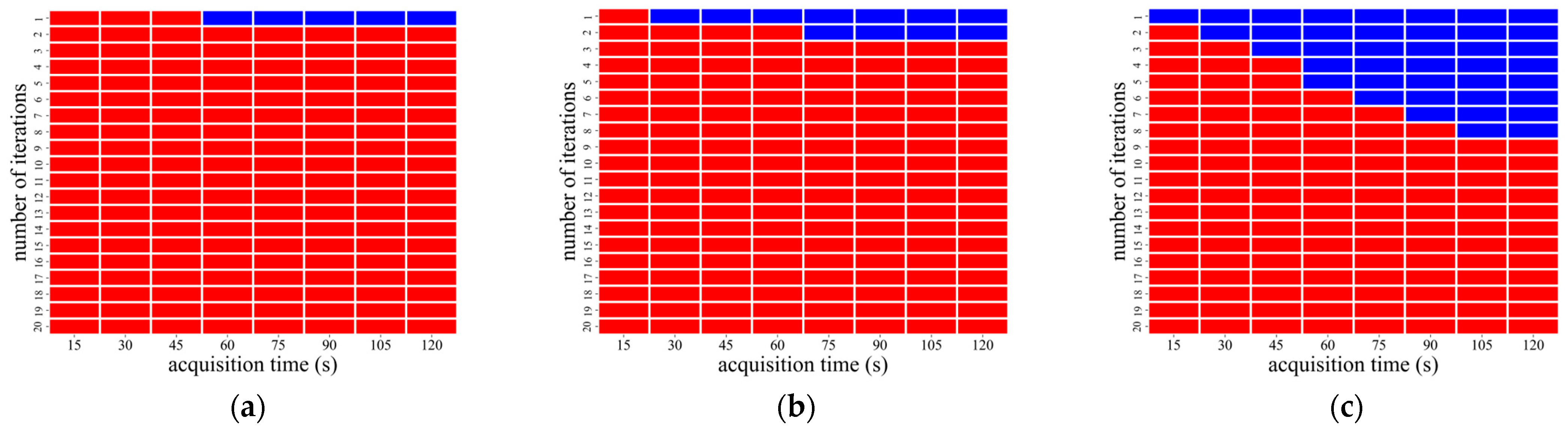
Figure 7 shows the N10mm results reconstructed using OSEM with TOF, and Figure 8 shows those reconstructed using OSEM with TOF and PSF. For OSEM with TOF reconstruction, N10mm exhibited similar trends among the Mild, Standard, and Strong CaLM settings. The recommended values could not be achieved using Mild. As the intensity of CaLM increased from Mild to Standard and Strong, more image reconstruction parameters were required to achieve the recommended values. A similar trend was observed for OSEM with TOF and PSF reconstruction. Compared to OSEM with TOF, OSEM with TOF and PSF reconstruction achieved the recommended values for more image reconstruction parameters. In both OSEM with TOF and OSEM with TOF and PSF reconstruction, the recommended values were achieved as the acquisition time increased.
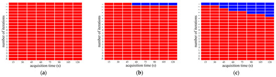
Figure 7.
N10mm results from OSEM with TOF reconstruction. (a–c) Mild, Standard, and Strong CaLM settings. In the figure, red indicates image reconstruction conditions that did not meet the guideline-recommended criteria, while blue indicates those that did (N10mm < 5.6%).
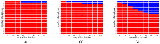
Figure 8.
N10mm results from OSEM with TOF and PSF reconstruction. (a–c) Mild, Standard, and Strong CaLM settings. In the figure, red indicates image reconstruction conditions that did not meet the guideline’s recommended criteria, while blue indicates those that did (N10mm < 5.6%).
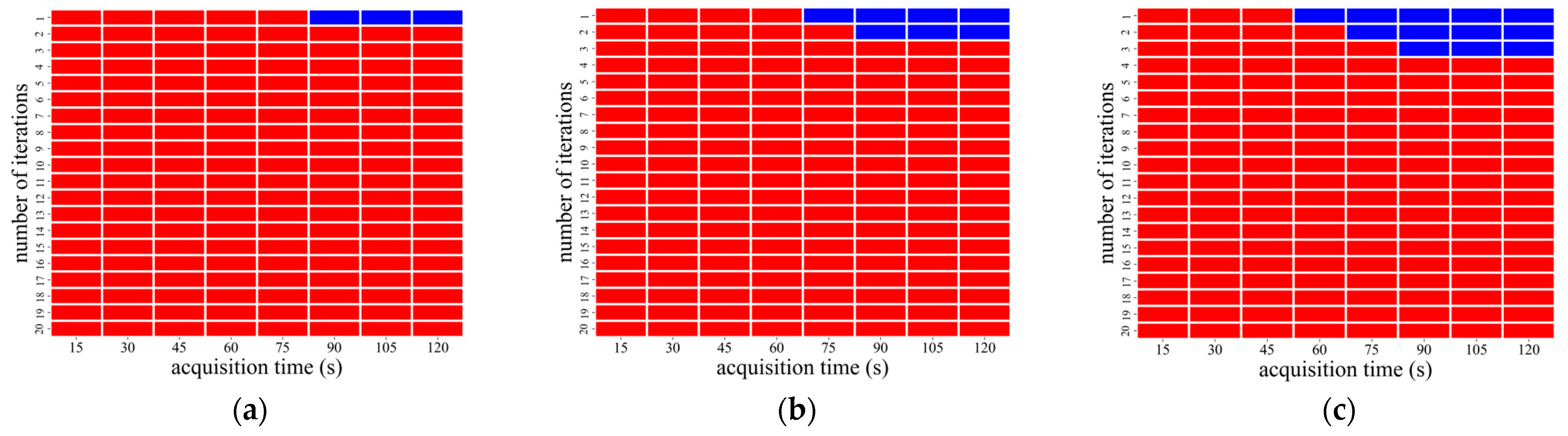
Figure 9 shows the QH10mm/N10mm results reconstructed using OSEM with TOF, and Figure 10 shows those reconstructed using OSEM with TOF and PSF. For OSEM with TOF reconstruction, QH10mm/N10mm exhibited similar trends among the Mild, Standard, and Strong CaLM settings. As the intensity of CaLM increased from Mild to Standard and Strong, QH10mm/N10mm showed a tendency to increase. For the same acquisition time, QH10mm/N10mm was more likely to achieve the recommended values when the CaLM intensity was higher. Similar trends were observed for OSEM with TOF and PSF reconstruction. Compared with OSEM with TOF reconstruction, OSEM with TOF and PSF reconstruction achieved the recommended values under more image reconstruction conditions. In both OSEM with TOF reconstruction and OSEM with TOF and PSF reconstructions, the recommended values were achieved as the acquisition time increased.
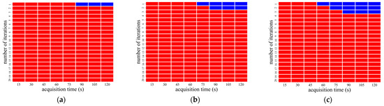
Figure 9.
QH10mm/N10mm results from OSEM with TOF reconstruction. (a–c) Mild, Standard, and Strong CaLM settings. In the figure, red indicates image reconstruction conditions that did not meet the guideline’s recommended criteria, while blue indicates those that did (QH10mm/N10mm > 2.8%).
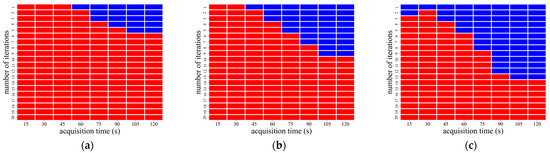
Figure 10.
QH10mm/N10mm results from OSEM with TOF and PSF reconstruction. (a–c) Mild, Standard, and Strong CaLM settings. In the figure, red indicates image reconstruction conditions that did not meet the guideline’s recommended criteria, while blue indicates those that did (QH10mm/N10mm > 2.8%).
Table 2 and Table 3 list the reconstruction parameters that achieved all physical indices when using OSEM with TOF and OSEM with TOF and PSF reconstruction. In OSEM with TOF reconstruction, the use of CaLM Mild did not allow for the simultaneous achievement of all physical indices. Additionally, when using Standard and Strong, a collection time of 75 s or more was necessary to simultaneously achieve all physical indices. Increasing the acquisition time enabled the gradual setting of a higher number of iterations to achieve the recommended values. In OSEM with TOF and PSF reconstruction, the reconstruction parameters that achieved all the recommended values simultaneously were Mild, Standard, and Strong. Using Mild, the recommended values could be achieved even with an acquisition time of 60 s. Furthermore, using Standard or Strong, the recommended values could be achieved with an acquisition time of less than 60 s. PSF correction showed a tendency to achieve the recommended values at higher iteration numbers compared to OSEM with TOF reconstruction.
Table 2.
Acquisition times and image reconstruction parameters that achieved all physical indices (CV, RC, N10mm and QH10mm/N10mm) with OSEM with TOF reconstruction.
Table 3.
Acquisition times and image reconstruction parameters that achieved all physical indices (CV, RC, N10mm, and QH10mm/N10mm) with OSEM with TOF and PSF reconstruction.
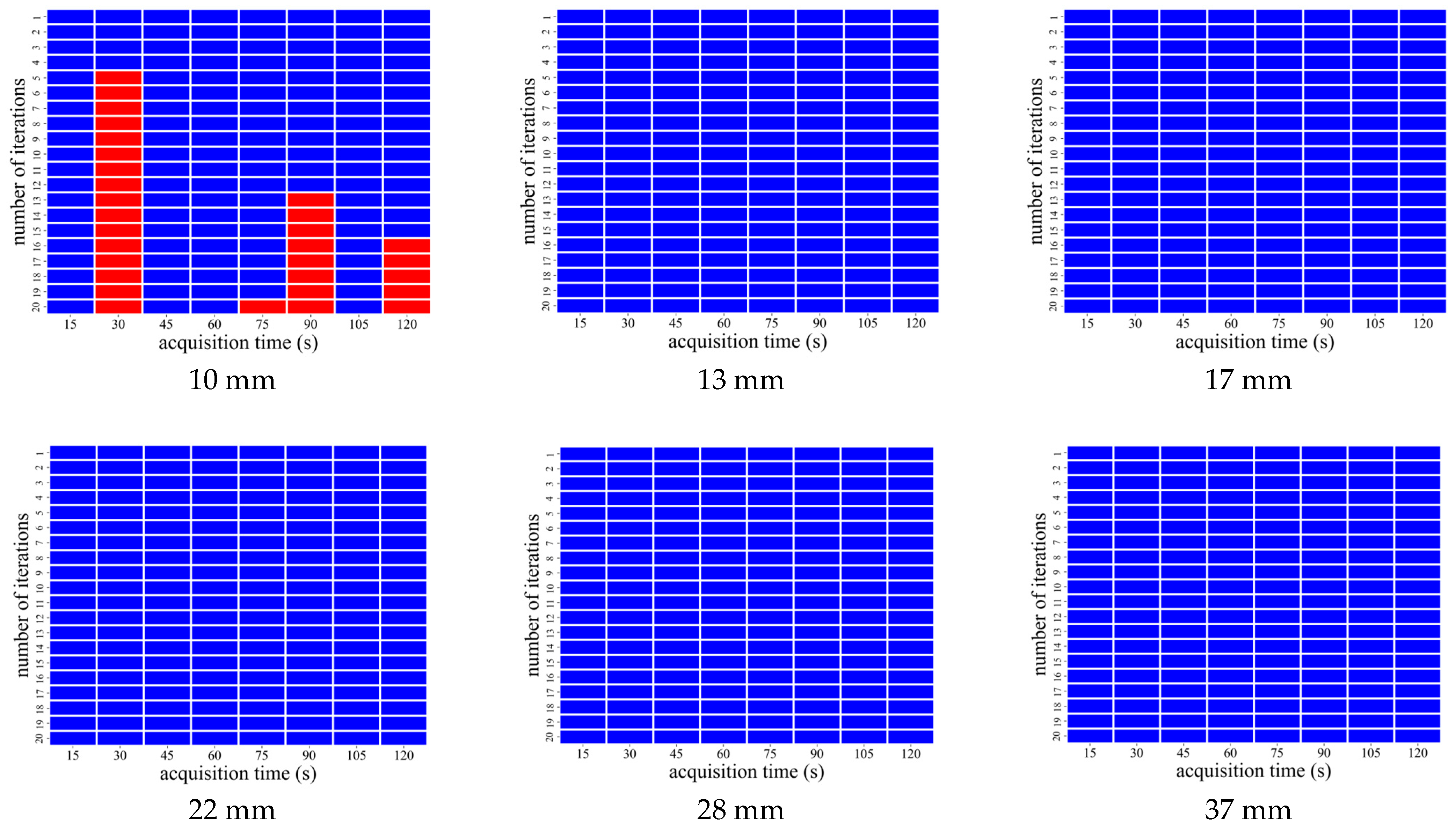
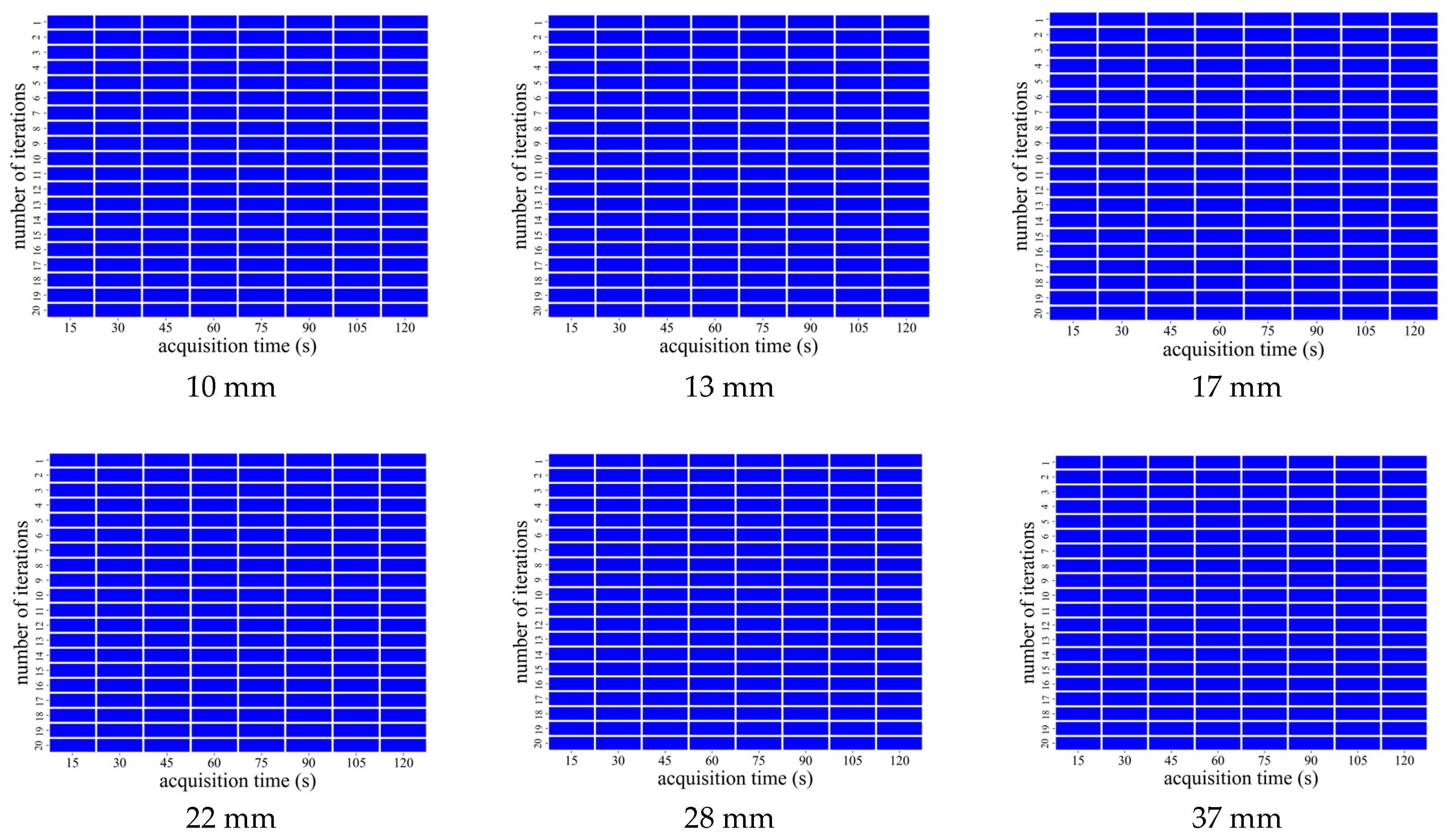
Figure 11, Figure 12 and Figure 13 show the results of CNR in the OSEM with TOF reconstruction. Specifically, Figure 11, Figure 12 and Figure 13 show the results for Mild, Standard, and Strong, respectively. When the hot sphere size was 13 mm or larger, all reconstruction parameters (e.g., iteration and CaLM) tended to satisfy the Rose criterion. However, for the 10 mm sphere, the reference values were not achieved for certain image reconstruction parameters, particularly when the iteration number was 5 or higher, depending on the acquisition time.
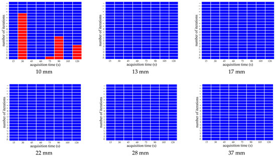
Figure 11.
Results of contrast-to-noise ratio (CNR) using CaLM Mild. In the figure, red indicates image reconstruction conditions that did not meet the Rose criterion, while blue indicates those that did (CNR > 5).
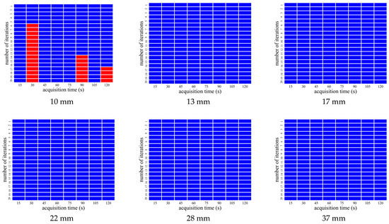
Figure 12.
Results of CNR using CaLM Standard. In the figure, red indicates image reconstruction conditions that did not meet the Rose criterion, while blue indicates those that did (CNR > 5).
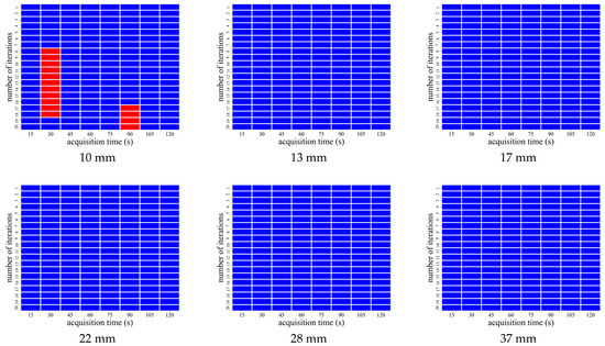
Figure 13.
Results of CNR using CaLM Strong. In the figure, red indicates image reconstruction conditions that did not meet the Rose criterion, while blue indicates those that did (CNR > 5).
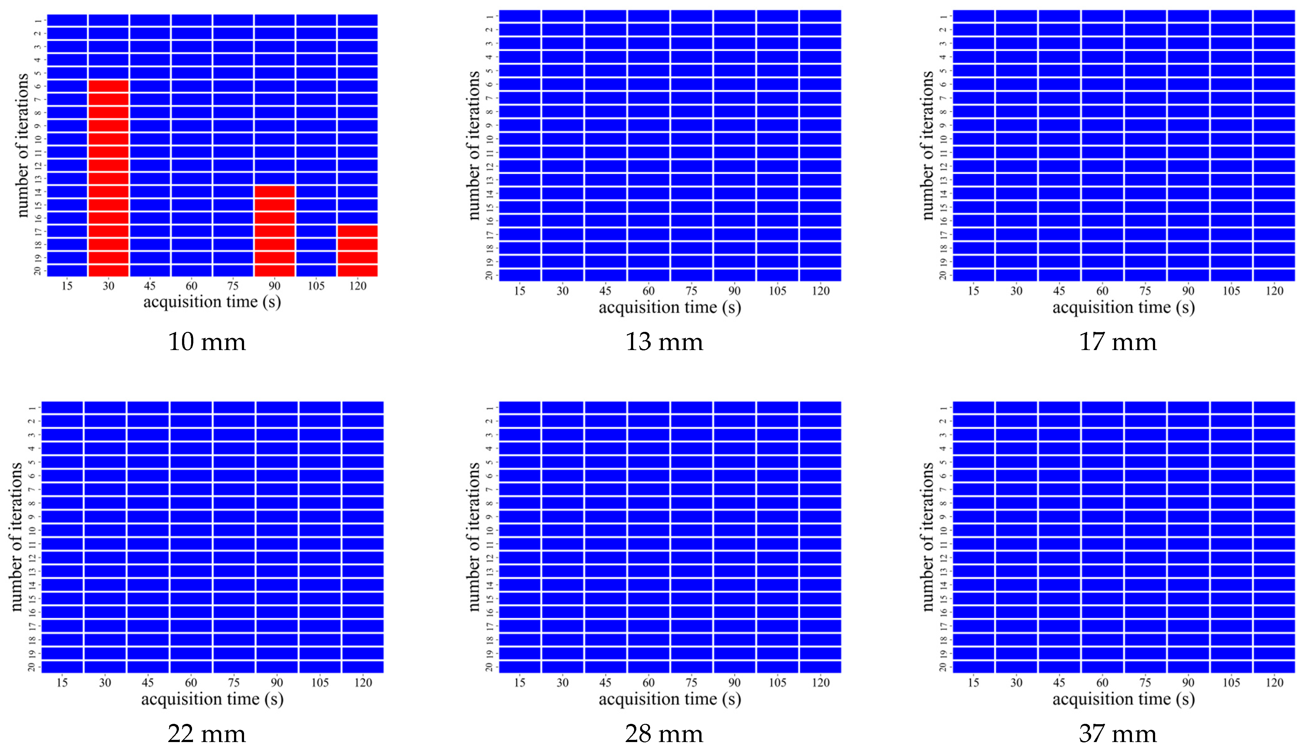
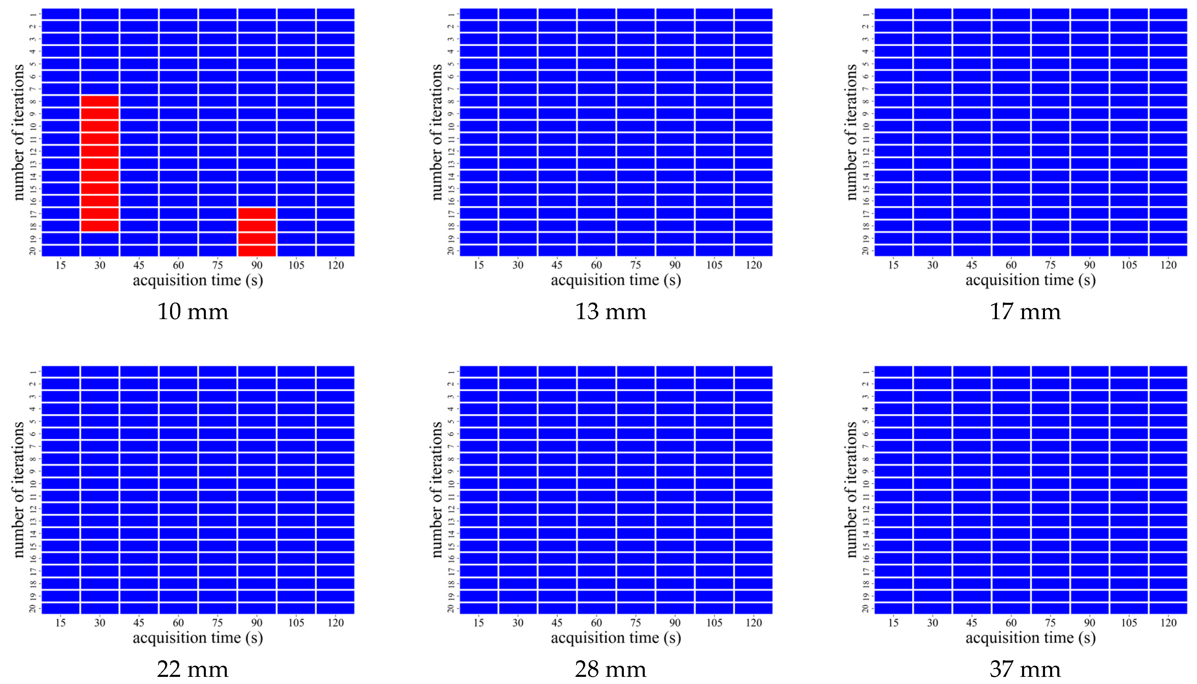
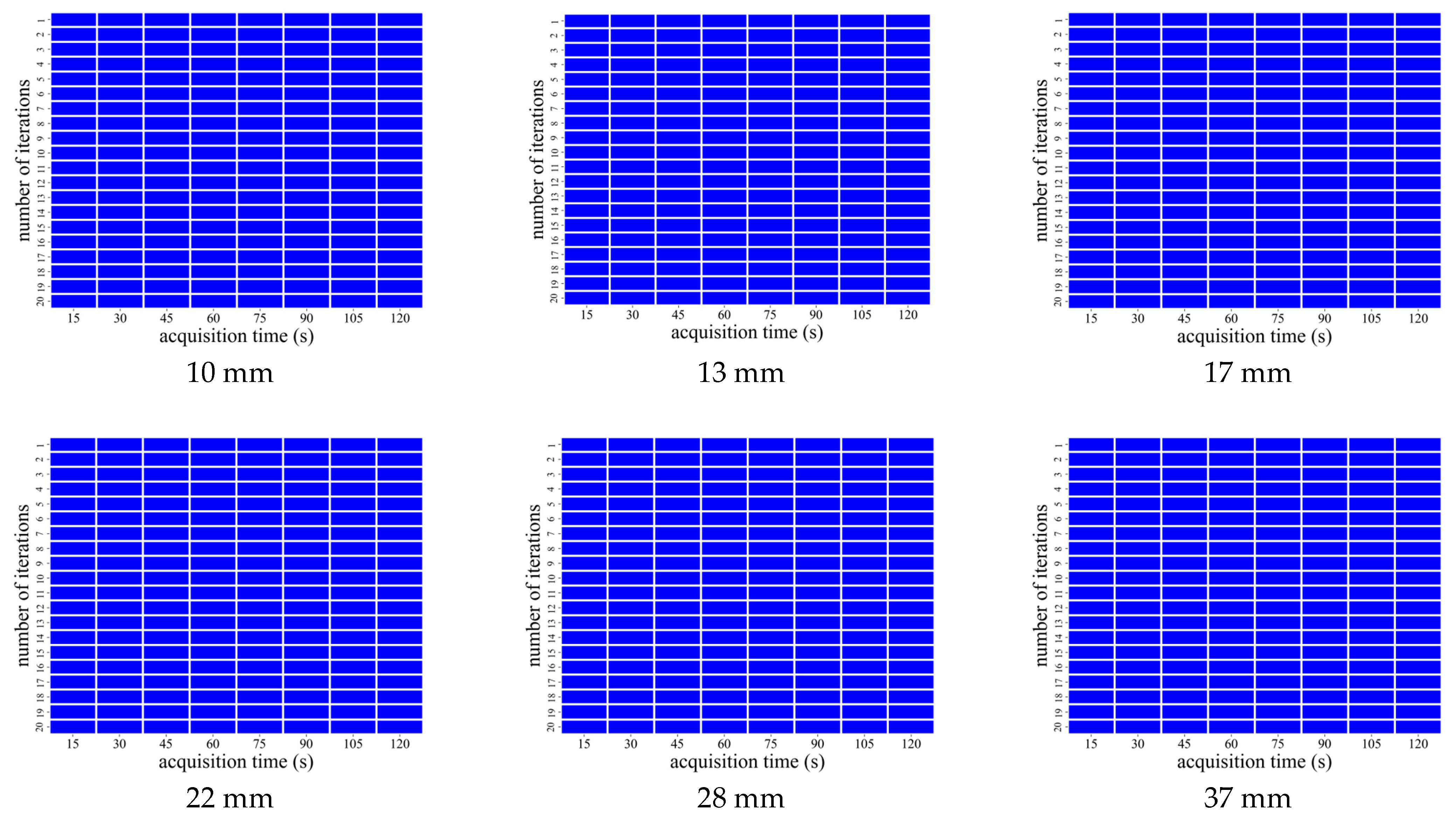
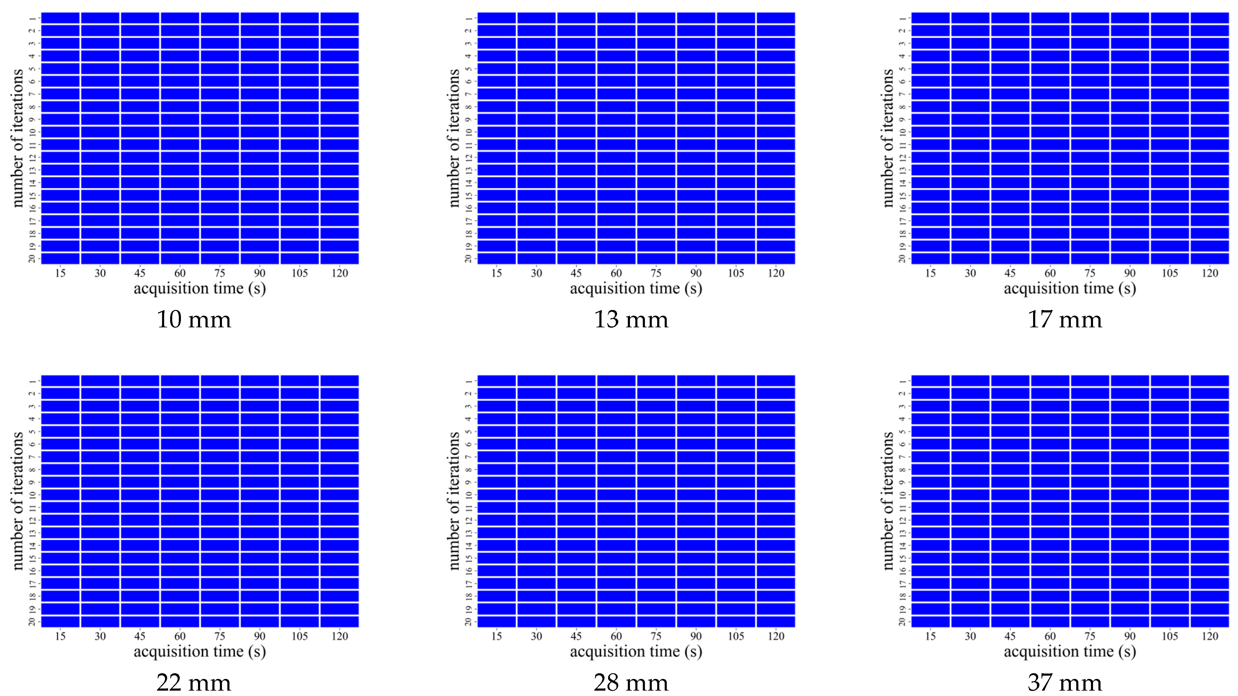
Figure 14, Figure 15 and Figure 16 show the results of CNR in the OSEM with TOF and PSF reconstruction. Specifically, Figure 14, Figure 15 and Figure 16 show the results for Mild, Standard, and Strong, respectively. Unlike in OSEM with TOF reconstruction, the Rose criterion was satisfied for all reconstruction parameters, even when the size of the hot sphere was 10 mm. Additionally, as the intensity of CaLM and acquisition time increased, the CNR values tended to increase.
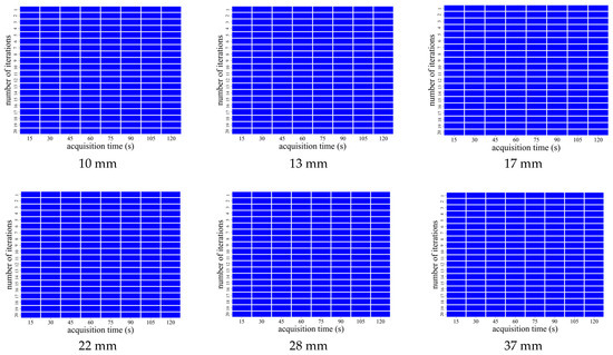
Figure 14.
Results of CNR using CaLM Mild. In the figure, red indicates image reconstruction conditions that did not meet the Rose criterion, while blue indicates those that did (CNR > 5).
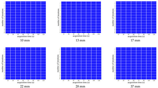
Figure 15.
Results of CNR using CaLM Standard. In the figure, red indicates image reconstruction conditions that did not meet the Rose criterion, while blue indicates those that did (CNR > 5).
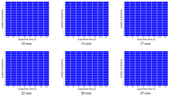
Figure 16.
Results of CNR using CaLM Strong. In the figure, red indicates image reconstruction conditions that did not meet the Rose criterion, while blue indicates those that did (CNR > 5).
3.2. AiCE Reconstruction
Table 4 presents the results for CV, RC, N10mm, QH10mm/N10mm, and CNR with AiCE reconstruction. In AiCE reconstruction, no physical parameters achieved the recommended values at an acquisition time of 15 s. When the acquisition time was 30 s or longer, CV achieved the recommended values. At 45 s or longer, RC and QH10mm/N10mm achieved the recommended values. However, N10mm did not achieve the recommended value at any acquisition time. Therefore, in AiCE reconstruction, achieving all indicators simultaneously was not possible.
Table 4.
Results of physical indices for Advanced intelligent Clear-IQ Engine (AiCE) reconstruction.
3.3. Visual Evaluation with AiCE Reconstruction
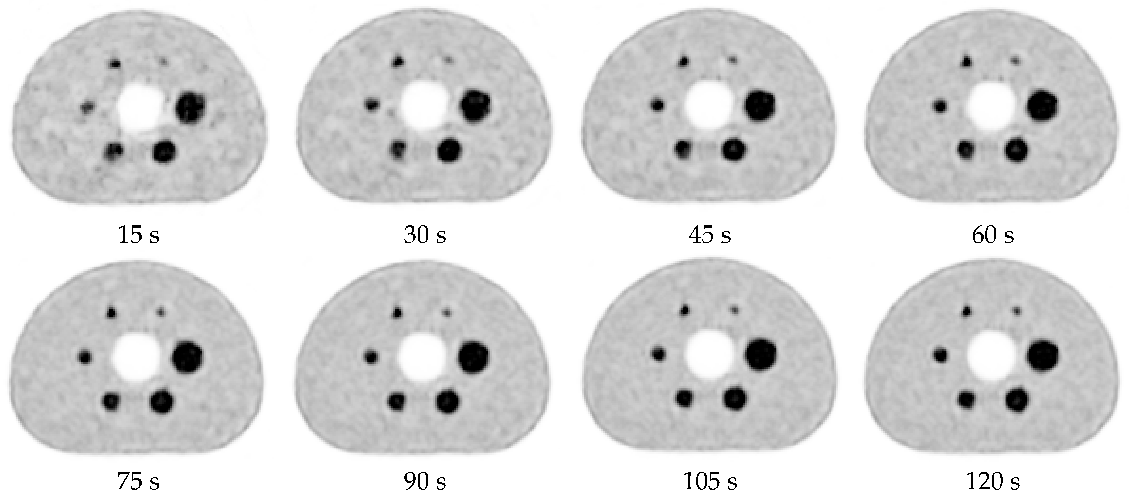
Figure 17 shows the image obtained using AiCE reconstruction, and Table 5 presents the results of the visual evaluation using AiCE reconstruction. The evaluation was performed by two radiological technologists with over five years of experience in nuclear medicine examination. According to Table 5, the scores for 10 mm sphere visualization, overall image quality, and image noise tended to improve as the acquisition time increased. Small signals, such as the 10 mm spheres, appeared difficult to visualize at acquisition times of 15 s and 30 s but became progressively easier to discern at 45 s or longer. Similarly, overall image quality was perceived to improve gradually at acquisition times of 45 s or longer. Image noise tended to decrease at acquisition times of 60 s or longer.
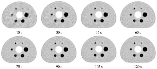
Figure 17.
Images obtained using AiCE reconstruction.
Table 5.
Visual evaluation with AiCE reconstruction.
4. Discussion
In this study, we verified the characteristics of short acquisition times using a SiPM-based semiconductor PET/CT system.
CaLM is considered to be based on the NLM method, which measures the similarity between the target pixel and the template window within the support window [6]. Therefore, it is expected to exhibit a similar trend across the Mild, Standard, and Strong levels. However, the intensity used during filter application (e.g., coefficients) is thought to differ among these levels. Additionally, for the aforementioned reason, images with a high level of noise may exhibit increased similarity, and as a result, the noise reduction effect may depend solely on the filter intensity. For these reasons, as the noise reduction effect of the filter increases with the Mild, Standard, and Strong levels, it is thought that the recommended values for CV, N10mm, and QH10mm/N10mm are more likely to be achieved (Figure 3, Figure 7 and Figure 9). On the other hand, it is thought that the increased noise reduction effect of the filter leads to signal reduction in RC (Figure 5).
Data acquisition over a short period of time leads to noise due to the radioactive decay of 18F and the number of photons incident on the detector. A phenomenon of noise divergence is observed when the iteration parameters are set too high. Increasing the amount of noise within the image in this way can inhibit the noise reduction effect of CaLM. Therefore, during short acquisition times, noise reduction was not effectively performed with Mild, Standard, and Strong, and the recommended values for CV, N10mm, and QH10mm/N10mm were not met (Figure 3, Figure 7 and Figure 9). On the other hand, since Mild has a lower noise reduction effect compared to Standard and Strong, it is thought that the recommended value for RC could still be met even with short acquisition times (Figure 5).
PSF correction is known to significantly improve image quality compared to image reconstruction methods without PSF correction [24], as the PSF algorithm includes additional information about the object to be recovered, which in turn significantly reduces noise levels [25,26]. Figure 4, Figure 6, Figure 8 and Figure 10 show that, when PSF correction is applied, there are more conditions that meet the recommended values compared to when no PSF correction is performed. The images with PSF correction exhibit less noise, and it is thought that applying CaLM further effectively reduces the noise. As such, applying PSF correction increases the number of conditions that meet the recommended values. However, caution is required when applying PSF correction, as Gibbs artifacts can lead to the overestimation of the signal intensity at the edges of the uptake regions [27,28].
Table 4 shows that in AiCE reconstruction, it was not possible to achieve all indicators simultaneously. AiCE reconstruction effectively reduces noise by using noise-free images (acquired with longer acquisition times) as training data [10]. Consequently, as the acquisition time increases, the CV value decreases, and the image noise in visual evaluation tends to receive higher scores. Moreover, AiCE reconstruction performs residual learning between the training data and the acquired images to reconstruct the images. As a result, metrics related to noise reduction, such as CV, N10mm, and QH10mm/N10mm, tended to achieve the recommended values more easily with longer acquisition times. Additionally, regarding the visibility of the 10 mm sphere, it is presumed that as the acquisition time increased, noise around the 10 mm sphere was effectively reduced, leading to a tendency for higher scores. Yamagiwa et al. reported that AiCE images exhibited significantly higher visual quality compared to OSEM images at an acquisition time of 90 s/bed [10]. Although this study did not compare AiCE images with conventional PET images, similar scores were observed at 90 s/bed. Furthermore, in this study, images at 75 s/bed achieved scores comparable to those at 90 s/bed in terms of 10 mm sphere visualization, overall image quality, and image noise. Since neither of them achieved all the recommended values, the decision to use one over the other should be made based on a balance between physical parameters and visual evaluation. Furthermore, AI technology is not limited to Canon but is incorporated into various manufacturers’ systems, resulting in differences in the effects achieved. In fact, Weyts, K et al. reported that it is possible to shorten the acquisition time to 45 s [29], which differs from the results reported by Elin et al. [30]. Since AiCE uses long-duration images as learning data and performs residual processing, a certain amount of acquisition time may be necessary. Therefore, it is not possible to directly apply the data from the various reports as they are. Users need to collect the base data and then adapt the clinical images based on these data.
Previous attempts to achieve short acquisition times have focused solely on reducing the acquisition duration, without considering reconstruction parameters. Pedro et al. reported [16] that it is possible to shorten the acquisition time to as little as 60 s not only by simply reducing the acquisition duration but also by adjusting the image reconstruction parameters. Although this appears to differ from the results of our study, it is presumed that the discrepancy arises from differences in the equipment used. These differences indicate that each PET/CT system has its own characteristics, and therefore, our findings may not be directly applicable to all systems. Accordingly, it is essential to have a thorough understanding of the specific characteristics of each PET/CT device when conducting examinations.
5. Conclusions
The characteristics of a short acquisition time were investigated using CaLM and AiCE reconstruction.
While a significant reduction in acquisition time was not achievable with OSEM with TOF reconstruction alone, the addition of PSF correction suggests the potential for a further reduction in acquisition time.
Although AiCE reconstruction did not achieve all recommended values simultaneously, no substantial discrepancy was observed between the calculated values and recommended thresholds. The use of AiCE reconstruction with a thorough understanding of its characteristics is considered essential.
Given that the characteristics of a short acquisition time are likely to vary depending on the equipment used, further investigation is required.
A limitation of this study is that it was conducted using phantom validation, not clinical data. In the future, it will be necessary to aim for clinical application based on the data obtained in this study.
Author Contributions
Conceptualization, R.O., K.K. and Y.T.; methodology, R.O., A.I. and T.H.; investigation, R.O. and A.I.; writing—original draft preparation, R.O.; writing—review and editing, T.H., S.H., Y.W., K.K., K.T., T.K., K.O. and Y.T.; supervision, R.O. and Y.T.; project administration, R.O. and Y.T. All authors have read and agreed to the published version of the manuscript.
Funding
This research received no external funding.
Institutional Review Board Statement
This study was conducted using a phantom and did not require institutional review board (or Ethics Committee) approval.
Informed Consent Statement
Not applicable.
Data Availability Statement
The data presented in this study are available in this article.
Conflicts of Interest
Tomoya, H. is an employee of PDRadio Pharma Company, Incorporated. The other authors declare no conflicits of interest.
References
- Fukukita, H.; Suzuki, K.; Matsumoto, K.; Terauchi, T.; Daisaki, H.; Ikari, Y.; Shimada, N.; Senda, M. Japanese guideline for the oncology FDG-PET/CT data acquisition protocol: Synopsis of Version 2.0. Ann. Nucl. Med. 2014, 28, 693–705. [Google Scholar] [CrossRef]
- Fletcher, J.W.; Djulbegovic, B.; Soares, H.P.; Siegel, B.A.; Lowe, V.J.; Lyman, G.H.; Coleman, R.E.; Wahl, R.; Paschold, J.C.; Avril, N.; et al. Recommendations on the use of 18F-FDG PET in oncology. J. Nucl. Med. 2008, 49, 480–508. [Google Scholar] [CrossRef] [PubMed]
- Yang, H.; Chen, S.; Qi, M.; Chen, W.; Kong, Q.; Zhang, J.; Song, S. Investigation of PET image quality with acquisition time/bed and enhancement of lesion quantification accuracy through deep progressive learning. EJNMMI Phys. 2024, 11, 7. [Google Scholar] [CrossRef]
- Chan, C.; Fulton, R.; Barnett, R.; Feng, D.D.; Meikle, S. Postreconstruction nonlocal means filtering of whole-body PET with an anatomical prior. IEEE. Trans Med. Imaging 2014, 33, 636–650. [Google Scholar] [CrossRef] [PubMed]
- Shirakawa, Y. Effect of low-dose 18F-FDG on image quality in digital PET/CT. Res. Sq. 2022, 11, 1–19. [Google Scholar] [CrossRef]
- Buades, B.; Coll, J.; Morel, M. A non-local algorithm for image denoising. In Proceedings of the IEEE Computer Society Conference on Computer Vision and Pattern Recognition (CVPR’05), San Diego, CA, USA, 20–25 June 2005; Volume 2, pp. 60–65. [Google Scholar] [CrossRef]
- Chan, C.; Meikle, S.; Fulton, R.; Tian, G.J.; Cai, W.; Feng, D.D. A non-local post-filtering algorithm for PET incorporating anatomical knowledge. In Proceedings of the IEEE Nuclear Science Symposium Conference Record (NSS/MIC), Orlando, FL, USA, 24 October–1 November 2009; pp. 2728–2732. [Google Scholar] [CrossRef]
- Dutta, J.; Leahy, R.M.; Li, Q. Non-local means denoising of dynamic PET images. PLoS ONE 2013, 8, e81390. [Google Scholar] [CrossRef]
- Inomata, T.; Sato, K.; Ibaraki, M.; Kominami, M.; Kinoshita, F.; Shinohara, Y.; Kato, M.; Kinoshita, T. Evaluation of low-dose whole-body FDG PET with SiPM-based PET/CT scanner: Visual and semi-quantitative analyses using random sampling from full-dose scan data. Jpn. J. Radiol. Technol. 2023, 79, 1127–1135. [Google Scholar] [CrossRef] [PubMed]
- Yamagiwa, K.; Tsuchiya, J.; Yokoyama, K.; Watanabe, R.; Kimura, K.; Kishino, M.; Tateishi, U. Enhancement of 18F-fluorodeoxyglucose PET image quality by deep-learning-based image reconstruction using advanced intelligent clear-IQ engine in semiconductor-based PET/CT scanners. Diagnostics 2022, 12, 2500. [Google Scholar] [CrossRef]
- Li, M.; Cui, X.; Yue, H.; Ma, C.; Li, K.; Chai, L.; Ge, M.; Li, H.; Ng, Y.L.; Zhou, Y.; et al. The efficacy of short acquisition time using 18F-FDG total-body PET/CT for the identification of pediatric epileptic foci. EJNMMI Res. 2024, 14, 21. [Google Scholar] [CrossRef]
- Zhang, Y.Q.; Hu, P.C.; Wu, R.Z.; Gu, Y.S.; Chen, S.G.; Yu, H.J.; Wang, X.Q.; Song, J.; Shi, H.C. The image quality, lesion detectability, and acquisition time of 18F-FDG total-body PET/CT in oncological patients. Eur. J. Nucl. Med. Mol Imaging 2020, 47, 2507–2515. [Google Scholar] [CrossRef]
- Alberts, I.; Sachpekidis, C.; Prenosil, G.; Viscione, M.; Bohn, K.P.; Mingels, C.; Shi, K.; Ashar-Oromieh, A.; Rominger, A. Digital PET/CT allows for shorter acquisition protocols or reduced radiopharmaceutical dose in [18F]-FDG PET/CT. Ann. Nucl. Med. 2021, 35, 485–492. [Google Scholar] [CrossRef] [PubMed]
- Sonni, I.; Baratto, L.; Park, S.; Hatami, N.; Srinivas, S.; Davidzon, G.; Gambhir, S.S.; Iagaru, A. Initial experience with a SiPM-based PET/CT scanner: Influence of acquisition time on image quality. EJNMMI Phys. 2018, 5, 9. [Google Scholar] [CrossRef] [PubMed]
- Pilz, J.; Hehenwarter, L.; Zimmermann, G.; Rendl, G.; Schweighofer-Zwink, G.; Beheshti, M.; Pirich, C. Feasibility of equivalent performance of 3D TOF [18F]-FDG PET/CT with reduced acquisition time using clinical and semiquantitative parameters. EJNMMI Res. 2021, 11, 44. [Google Scholar] [CrossRef]
- Fragoso Costa, P.; Jentzen, W.; Brahmer, A.; Mavroeidi, I.A.; Zarrad, F.; Umutlu, L.; Fendler, W.P.; Rischpler, C.; Herrmann, K.; Conti, M.; et al. Phantom-based acquisition time and image reconstruction parameter optimisation for oncologic FDG PET/CT examinations using a digital system. BMC Cancer 2022, 22, 899. [Google Scholar] [CrossRef]
- Alqahtani, M.M.; Willowson, K.P.; Constable, C.; Fulton, R.; Kench, P.L. Optimization of 99mTc whole-body SPECT/CT image quality: A phantom study. J. Appl Clin. Med Phys. 2022, 23, e13528. [Google Scholar] [CrossRef] [PubMed]
- Zhao, J.; Liu, Q.; Li, C.; Song, Y.; Zhang, Y.; Chen, J.C. Optimization of spatial resolution and image reconstruction parameters for the small-animal Metis™ PET/CT system. Electronics 2022, 11, 1542. [Google Scholar] [CrossRef]
- Emura, R. [[PET] 6. Overview of clinical applications of artificial intelligence in PET]. Jpn. J. Radiol. Technol. 2023, 79, 595–606. [Google Scholar] [CrossRef]
- Shehata, M.A.; Saad, A.M.; Kamel, S.; Stanietzky, N.; Roman-Colon, A.M.; Morani, A.C.; Elsayes, K.M.; Jensen, C.T. Deep-learning CT reconstruction in clinical scans of the abdomen: A systematic review and meta-analysis. Abdom. Radiol. 2023, 48, 2724–2756. [Google Scholar] [CrossRef]
- Mori, M.; Fujioka, T.; Hara, M.; Katsuta, L.; Yashima, Y.; Yamaga, E.; Yamagiwa, K.; Tsuchiya, J.; Hayashi, K.; Kumaki, Y.; et al. Deep Learning-Based Image Quality Improvement in Digital Positron Emission Tomography for Breast Cancer. Diagnostics 2023, 13, 794. [Google Scholar] [CrossRef]
- Tsuchiya, J.; Yokoyama, K.; Yamagiwa, K.; Watanabe, R.; Kimura, K.; Kishino, M.; Chan, C.; Asma, E.; Tateishi, U. Deep learning-based image quality improvement of 18F-fluorodeoxyglucose positron emission tomography: A retrospective observational study. EJNMMI Phys. 2021, 8, 31. [Google Scholar] [CrossRef]
- Huizing, D.M.V.; Sinaasappel, M.; Dekker, M.C.; Stokkel, M.P.M.; de Wit-van der Veen, B.J. 177 Lutetium SPECT/CT: Evaluation of collimator, photopeak and scatter correction. J. Appl. Clin. Med. Phys. 2020, 21, 272–277. [Google Scholar] [CrossRef] [PubMed]
- Hausmann, D.; Dinter, D.J.; Sadick, M.; Brade, J.; Schoenberg, O.S.; Büsing, K. The impact of acquisition time on image quality in whole-body 18F-FDG PET/CT for cancer staging. J. Nucl. Med. Technol. 2012, 40, 255–258. [Google Scholar] [CrossRef] [PubMed]
- Taniguchi, T.; Akamatsu, G.; Kasahara, Y.; Mitsumoto, K.; Baba, S.; Tsutsui, Y.; Himuro, K.; Mikasa, S.; Kidera, D.; Sasaki, M. Improvement in PET/CT image quality in overweight patients with PSF and TOF. Ann. Nucl. Med. 2015, 29, 71–77. [Google Scholar] [CrossRef] [PubMed]
- Akamatsu, G.; Ishikawa, K.; Mitsumoto, K.; Taniguchi, T.; Ohya, N.; Baba, S.; Abe, K.; Sasaki, M. Improvement in PET/CT image quality with a combination of point-spread function and time-of-flight in relation to reconstruction parameters. J. Nucl. Med. 2012, 53, 1716–1722. [Google Scholar] [CrossRef]
- Rahmim, A.; Qi, J.; Sossi, V. Resolution modeling in PET imaging: Theory, practice, benefits, and pitfalls. Med. Phys. 2013, 40, 064301. [Google Scholar] [CrossRef]
- Nakamura, A.; Tanizaki, Y.; Takeuchi, M.; Ito, S.; Sano, Y.; Sato, M.; Kanno, T.; Okada, H.; Torizuka, T.; Nishizawa, S. Impact of point spread function correction in standardized uptake value quantitation for positron emission tomography images: A study based on phantom experiments and clinical images. Jpn. J. Radiol. Technol. 2014, 70, 542–548. [Google Scholar] [CrossRef]
- Weyts, K.; Lasnon, C.; Ciappuccini, R.; Lequesne, J.; Corroyer-Dulmont, A.; Quak, E.; Clarisse, B.; Roussel, L.; Bardet, S.; Jaudet, C. Artificial intelligence-based PET denoising could allow a two-fold reduction in [18F]FDG PET acquisition time in digital PET/CT. Eur. J. Nucl. Med. Mol. Imaging 2022, 49, 3750–3760. [Google Scholar] [CrossRef]
- Trägårdh, E.; Minarik, D.; Almquist, H.; Bitzén, U.; Garpered, S.; Hvittfelt, E.; Olsson, B.; Oddstig, J. Impact of acquisition time and penalizing factor in a block-sequential regularized expectation maximization reconstruction algorithm on a Si-photomultiplier-based PET-CT system for 18F-FDG. EJNMMI Res. 2019, 9, 64. [Google Scholar] [CrossRef]

Disclaimer/Publisher’s Note: The statements, opinions and data contained in all publications are solely those of the individual author(s) and contributor(s) and not of MDPI and/or the editor(s). MDPI and/or the editor(s) disclaim responsibility for any injury to people or property resulting from any ideas, methods, instructions or products referred to in the content. |
© 2025 by the authors. Licensee MDPI, Basel, Switzerland. This article is an open access article distributed under the terms and conditions of the Creative Commons Attribution (CC BY) license (https://creativecommons.org/licenses/by/4.0/).