Comparison between Calculation and Measurement of Total Sediment Load: Application to Nestos River ^†

Abstract

Measurements of stream discharge, bed load transport rate and suspended sediment concentration in the Nestos River (northeastern Greece) were conducted by the Section of Hydraulic Engineering, of the Civil Engineering Department, Democritus University of Thrace. In addition to those measurements, the total sediment concentration was calculated by means of the formulas of Yang. The comparison between the calculated and measured total sediment concentration was achieved by means of several statistical criteria and the results were deemed satisfactory.

1. Introduction

Stream sediment transport still stands out as a challenging problem for hydraulic engineers. Despite the leaps that have been made in the last century in the understanding and modeling of river load transport, the problem remains largely unintelligible and insoluble, due to the complexity of the physical processes that describe it.

Sediment transport affects riverine systems, either directly or indirectly, through erosion and deposition. Excessive depositions, as a result of soil erosion, affect the cross sections, increase the risk of flooding and can lead to a deterioration of water quality. This problem can be exacerbated in the case of agricultural basins where sediments may be carriers of infectious particles due to the use of fertilizers and pesticides [1].

Total sediment transport in streams is classified into bed load transport and suspended load transport on the basis of two different motion patterns. The sum of bed load and suspended load is equal to the total load [2].

In the recent decades, the Section of Hydraulic Engineering of the Civil Engineering Department, Democritus University of Thrace (Greece), has conducted bed load transport rate measurements and suspended sediment concentration measurements at the outlet of the Nestos River basin [3], Kosynthos River basin [4,5], and Kimmeria Torrent basin [5].

This study aims to redetermine the coefficients of Yang’s (1973) and Yang’s (1979) sediment transport formulas using multiple regression. In the past, nonlinear regression equations between bed load transport rate and stream flow rate, as well as between suspended load transport rate and stream flow rate, were established for the outlet of the Nestos River basin [3]. In the present study, 111 pairs of measured stream flow rate, measured bed load transport rate or measured suspended load transport rate in the Nestos River were used. The sum of measured bed load transport rate and measured suspended load transport rate provides the measured total load transport rate from which the total sediment concentration can be estimated. Apart from those measurements, total sediment concentrations were calculated by means of Yang’s formulas [6,7]. This made it possible to compare calculated to site-measured total sediment concentrations.

2. Study Area

The Nestos River springs from the Rila Mountains in southwestern Bulgaria and is one of the main watercourses of Eastern Macedonia and Thrace (Greece). Its Greek part covers approximately 130 km and the mountainous part of the Nestos River basin extends to an area of 840 km². The basin is covered by forest (48%), bush (20%), cultivated land (24%), urban area (2%) and areas of no significant vegetation (6%), and has an altitude between 38 m and 1747 m. The basin is divided into 20 sub-basins with coverage areas between 13 km² and 80 km² and the mean land slope is between 23% and 58%. The mean slope of the main streams of the sub-basins ranges between 2.5% and 20%, whereas the mean slope of the Nestos River is 0.35%.

3. Stream Flow Rate and Sediment Transport Rate Measurements

All measurements were conducted at a location between the outlet of the Nestos River basin (Toxotes) and the river’s delta [8,9]. The average width of the cross sections of all measurements is 26.7 m.

The stream flow rate measurements were conducted using the following procedure: the site cross section was divided into sub-sections and the average stream flow velocity was measured at the middle of each sub-section, at 40%, approximately, of the flow depth from the bed, using a Valeport open channel flow meter. The stream flow rate of the entire cross section was taken as the sum of the individual sub-sections stream flow rates.

The bed load transport rate measurements were conducted in the middle of each cross section using a Helley–Smith bed load sampler. In order to determine the bed load transport rate, the trapped bed load sample is dried out and the mass is divided by the trap width and the measurement time duration [8,9].

The suspended sediment concentration was determined by obtaining a sample of water at the middle of the section and subsequently filtrating the sample through retention paper filters to obtain the net weight of the suspended load [8,9].

4. Calculation of Total Sediment Concentration

“Unit stream power”, as defined by Yang [6], is the amount of dynamic energy consumed by gravitational flow per unit of time and per unit weight of water, and is expressed by the product of the flow rate and the energy slope:

$$\frac{\mathrm{d}\mathrm{Y}}{\mathrm{d}\mathrm{t}}=\frac{\mathrm{d}\mathrm{x}}{\mathrm{d}\mathrm{t}}\frac{\mathrm{d}\mathrm{Y}}{\mathrm{d}\mathrm{x}}=\mathrm{u}\mathrm{s}=\mathrm{u}\mathrm{n}\mathrm{i}\mathrm{t}\mathrm{stream}\mathrm{power}$$

(1)

where Y is the elevation above a datum, equal to the potential energy per unit weight of water; x is the horizontal distance; and t is the time.

4.1. Yang (1973)

Yang’s [6] formula for the total sediment transport in a river is given by:

$$\log {\mathrm{c}}_{\mathrm{F}}=5.435-0.286\log \frac{\mathrm{w}{\mathrm{D}}_{50}}{\mathrm{v}}-0.457\log \frac{{\mathrm{u}}_{*}}{\mathrm{w}}+\left(1.799-0.409\log \frac{\mathrm{w}{\mathrm{D}}_{50}}{\mathrm{v}}-0.314\log \frac{{\mathrm{u}}_{*}}{\mathrm{w}}\right)\log \left(\frac{\mathrm{u}\mathrm{s}}{\mathrm{w}}-\frac{{\mathrm{u}}_{\mathrm{cr}}\mathrm{s}}{\mathrm{w}}\right)$$

(2)

where c_F is the total sediment concentration in parts per million (ppm) by weight; w is the terminal fall velocity of sediment particles (m/s); D₅₀ is the median particle diameter (m); ν is the kinematic viscosity of water (m²/s); s is the energy slope; u is the mean flow velocity (m/s); u_cr is the critical mean flow velocity (m/s); and u_* is the shear velocity (m/s).

If the following auxiliary variables ${\mathrm{x}}_1$, ${\mathrm{x}}_2$, ${\mathrm{x}}_3$, ${\mathrm{x}}_4$ and ${\mathrm{x}}_5$ are considered:

$$\begin{array}{l}{\mathrm{x}}_1=\log (\mathrm{w}\mathrm{D}50/\mathsf{\nu })\\ {\mathrm{x}}_2=\log ({\mathrm{u}}_{*}^{}/\mathrm{w})\\ {\mathrm{x}}_3=\log (\mathrm{u}\mathrm{s}/\mathrm{w}-\mathrm{ucr}\mathrm{s}/\mathrm{w})\\ {\mathrm{x}}_4=\log (\mathrm{u}\mathrm{s}/\mathrm{w}-\mathrm{ucr}\mathrm{s}/\mathrm{w})\log (\mathrm{w}\mathrm{D}50/\mathsf{\nu })\\ {\mathrm{x}}_5=\log (\mathrm{u}\mathrm{s}/\mathrm{w}-\mathrm{ucr}\mathrm{s}/\mathrm{w})\log ({\mathrm{u}}_{*}^{}/\mathrm{w})\end{array}$$

(3)

then Yang’s formula can be written as follows:

$$\log {\mathrm{c}}_{\mathrm{F}}=5.435-0.286{\mathrm{x}}_1-0.457{\mathrm{x}}_2+1.799{\mathrm{x}}_3-0.409{\mathrm{x}}_4-0.314{\mathrm{x}}_5$$

(4)

White et al. [10] calculated the terminal fall velocity of the particles using the following equations:

$$\mathrm{w}=\mathrm{F}\sqrt{{\mathsf{\rho }}^{\prime }\mathrm{g}\mathrm{D}}$$

(5)

$$\mathrm{F}=\sqrt{\left(\frac{2}{3}+\frac{36}{\mathrm{D}{*}^3}\right)}+\sqrt{\frac{36}{\mathrm{D}{*}^3}}$$

(6)

$$\mathrm{D}*=\sqrt[3]{\frac{{\mathsf{\rho }}^{\prime }\mathrm{g}}{{\mathsf{\nu }}^2}}{\mathrm{D}}_{\mathrm{ch}}$$

(7)

$${\mathsf{\rho }}^{\prime }=\frac{{\mathsf{\rho }}_{\mathrm{F}}-{\mathsf{\rho }}_{\mathrm{w}}}{{\mathsf{\rho }}_{\mathrm{w}}}$$

(8)

where F is the correction factor for suspended load; D is the grain diameter (m); D* is the Bonnefille number; D_ch is the characteristic grain diameter (m); ρ_F is the density of sediment particles (kg/m³); and ρ_W is the density of water (kg/m³). The kinematic viscosity v (m²/s) of water is given by the equation:

$$\mathsf{\nu }=\frac{1.78\times 10^{-6}}{1+0.0337\mathrm{T}+0.00022{\mathrm{T}}^2}$$

(9)

where T (°C) is the temperature of the water.

4.2. Yang (1979)

In 1979, Yang concluded that the critical unit stream power term in Equation (2) can be neglected without causing much error when the measured sediment concentration is greater than 20 ppm by weight [7]. The simplified unit stream power equation was derived as:

$$\log c_F=5.165-0.153\log \frac{w{D}_{50}}{v}-0.297\log \frac{u_{*}}{w}+\left(1.780-0.360\log \frac{w{D}_{50}}{v}-0.480\log \frac{u_{*}}{w}\right)\log \left(\frac{us}{w}\right)$$

(10)

Similarly, if the following auxiliary variables ${\mathrm{x}\prime }_1$, ${\mathrm{x}\prime }_2$, ${\mathrm{x}\prime }_3$, ${\mathrm{x}\prime }_4$ and ${\mathrm{x}\prime }_5$ are considered:

$$\begin{array}{l}{\mathrm{x}\prime }_1=\log (\mathrm{wD}50/\mathsf{\nu })\\ {\mathrm{x}\prime }_2{=\log (\mathrm{u}}_{*}^{}/\mathrm{w})\\ {\mathrm{x}\prime }_3=\log (\mathrm{us}/\mathrm{w})\\ {\mathrm{x}\prime }_4=\log (\mathrm{us}/\mathrm{w})\log (\mathrm{wD}50/\mathsf{\nu })\\ {\mathrm{x}\prime }_5{=\log (\mathrm{us}/\mathrm{w})\log (\mathrm{u}}_{*}^{}/\mathrm{w})\end{array}$$

(11)

Equation (10) can be written as a linear multiple regression equation:

$${\mathrm{logc}}_{\mathrm{F}}=5.165-0{.153\mathrm{x}\prime }_1-0{.297\mathrm{x}\prime }_2+1{.780\mathrm{x}\prime }_3-0{.360\mathrm{x}\prime }_4-0{.480\mathrm{x}\prime }_5$$

(12)

5. Development of Yang’s Equations on the Basis of Nestos River Data

On the basis of the Nestos River data, the arithmetic coefficients of the original formulas of Yang [6,7], (Equations (2) and (10)), are modified, respectively, as follows:

$${\mathrm{logc}}_{\mathrm{F}}=2.595-0.560\log \frac{{\mathrm{wD}}_{50}}{\mathrm{v}}-6.649\log \frac{{\mathrm{u}}_{*}}{\mathrm{w}}-\left(1.380-0.534\log \frac{{\mathrm{wD}}_{50}}{\mathrm{v}}+2.315\log \frac{{\mathrm{u}}_{*}}{\mathrm{w}}\right)\log \left(\frac{\mathrm{us}}{\mathrm{w}}-\frac{{\mathrm{u}}_{\mathrm{cr}}\mathrm{s}}{\mathrm{w}}\right)$$

(13)

$${\mathrm{logc}}_{\mathrm{F}}=3.301-0.697\log \frac{{\mathrm{wD}}_{50}}{\mathrm{v}}-14.367\log \frac{{\mathrm{u}}_{*}}{\mathrm{w}}-\left(1.214-0.537\log \frac{{\mathrm{wD}}_{50}}{\mathrm{v}}+7.301\log \frac{{\mathrm{u}}_{*}}{\mathrm{w}}\right)\log \left(\frac{\mathrm{us}}{\mathrm{w}}\right)$$

(14)

In concrete terms, the new arithmetic coefficients of Equations (13) and (14) were determined by means of the conventional least square-based regression.

The measured stream flow rate (m³/s), the measured total sediment concentration (ppm), as well as the corresponding calculated total sediment concentration (ppm), by means of Equations (13) and (14), are provided in Table 1.

Table 1. Measured stream flow rate and total sediment concentration—Calculated total sediment concentration in the Nestos River.

No.	Stream Flow Rate (m3/s)	Total Load logcF (meas.)	Total Load logcF (calc.) Yang 1973	Total Load logcF (calc.) Yang 1979	No.	Stream Flow Rate (m3/s)	Total Load logcF (meas.)	Total Load logcF (calc.) Yang 1973	Total Load logcF (calc.) Yang 1979
1	14.17	2.4064	2.3272	2.4124	31	3.16	2.4852	2.1243	2.1413
2	17.44	2.3929	2.2086	2.3058	32	2.56	1.6531	2.1818	2.1209
3	19.50	2.1160	2.1335	2.1819	33	3.95	2.0033	2.0120	2.0609
4	16.65	2.5769	2.2280	2.3020	34	4.22	2.1990	2.0149	2.0704
5	18.49	2.3163	2.1567	2.2284	35	3.66	2.3754	2.0099	2.0559
6	2.44	1.3789	2.0625	2.1273	36	4.80	2.2213	1.9135	1.9778
7	2.73	1.3806	1.9514	2.0150	37	2.06	2.0066	1.7068	1.7695
8	2.69	1.2852	1.9321	1.9866	38	1.46	2.2493	1.8468	1.9173
9	2.84	1.2712	1.8949	1.9532	39	1.88	2.1066	1.7164	1.7854
10	3.09	1.3444	1.9260	2.0052	40	1.49	2.1652	1.8366	1.9067
11	17.89	0.9300	1.3330	1.4140	41	1.75	2.1639	1.7815	1.8486
12	15.45	1.5009	1.4583	1.5803	42	1.66	1.7420	1.8333	1.9043
13	20.62	1.4076	1.2519	1.3096	43	2.29	1.7200	1.6467	1.7179
14	16.15	1.2719	1.4327	1.5588	44	1.55	2.1600	1.8386	1.8937
15	14.14	0.8808	1.5299	1.6691	45	1.24	1.8919	1.9283	1.9875
16	58.98	−0.4977	0.7454	0.4515	46	1.65	2.6312	1.7926	1.8650
17	52.94	0.3224	0.8856	0.7877	47	1.56	1.5917	1.8406	1.9286
18	50.14	1.0832	0.8405	0.5748	48	2.03	1.1085	1.7015	1.7641
19	48.27	0.6214	0.9100	0.7553	49	0.80	1.4741	1.9474	2.0033
20	45.72	0.5341	0.9570	0.8348	50	0.69	1.0102	1.9347	1.9919
21	44.45	0.9808	0.9586	0.7920	51	0.69	1.1868	2.0170	2.0654
22	62.41	1.2658	0.7342	0.4807	52	0.90	1.5753	1.8987	1.9769
23	55.30	0.5716	0.8122	0.5924	53	3.27	2.1887	1.9611	2.0192
24	2.62	2.6540	1.9164	1.9354	54	3.70	2.4867	1.7769	1.8147
25	3.95	2.6132	2.0149	2.0704	55	2.48	2.2356	2.0437	2.0747
26	4.22	2.5023	1.9973	2.0650	56	2.23	2.6100	2.0533	2.0860
27	4.13	2.4793	1.9776	2.0225	57	0.85	2.0211	2.3816	2.2171
28	6.20	2.4870	1.8488	1.9273	58	0.64	2.3324	2.0842	1.9663
29	4.80	2.6715	1.8485	1.8979	59	0.55	2.2624	2.3519	2.2803
30	3.76	2.5385	1.9707	2.0092	60	2.83	2.0921	1.9500	2.0009
61	3.40	2.2798	1.9355	1.9988	87	0.90	1.9402	2.0299	1.9359
62	3.29	2.0411	1.9162	1.9825	88	0.88	1.9007	1.6822	1.6011
63	1.77	2.7604	2.1373	2.1580	89	0.97	1.4280	1.8835	1.8606
64	1.06	2.7836	2.4887	2.3048	90	0.47	1.7540	2.2480	2.1496
65	0.60	2.5666	2.4785	2.1120	91	0.52	1.8291	2.3018	2.2275
66	0.39	2.3439	2.7624	2.3083	92	0.29	2.0208	2.3191	2.1865
67	0.64	2.8455	2.5643	2.2200	93	1.39	0.0803	2.2672	2.2396
68	2.67	1.6012	2.0161	2.0783	94	1.36	0.2972	2.0320	1.9492
69	3.68	2.0237	1.8693	1.9422	95	0.93	2.4222	2.7206	2.7267
70	2.45	1.7286	2.0470	2.0960	96	1.15	2.2505	2.5983	2.6155
71	2.62	2.5135	2.0109	2.0678	97	2.05	2.6852	2.3236	2.3769
72	2.95	2.5891	2.0145	2.0770	98	0.87	1.9359	2.2107	2.0739
73	0.84	1.7919	2.0595	2.0582	99	0.85	2.4092	2.7146	2.6828
74	1.76	1.4119	1.7486	1.8104	100	1.06	2.0224	2.1208	2.0151
75	1.81	2.0826	1.7312	1.7866	101	1.26	2.4699	2.2245	2.1058
76	1.09	2.2863	1.9924	2.0559	102	0.49	2.5759	2.1305	2.1176
77	0.59	2.3232	2.3234	2.2569	103	0.34	2.7771	2.3937	2.3719
78	1.06	2.2265	1.7887	1.8405	104	1.34	1.7905	1.9632	2.0090
79	0.75	2.3269	1.8485	1.8623	105	0.68	2.4427	2.1192	2.1378
80	1.43	2.2886	1.6653	1.7245	106	0.10	2.9859	1.9198	2.1113
81	1.47	1.8679	1.7191	1.7927	107	17.28	1.8167	1.5857	1.6423
82	0.64	2.1852	1.9814	1.9869	108	8.24	2.2106	2.0268	2.1808
83	0.55	1.4934	2.1193	1.9905	109	0.94	2.0663	1.8149	1.9314
84	0.83	1.9176	2.1437	2.0544	110	9.83	1.9549	1.7134	1.8098
85	0.85	1.7439	1.9873	1.9228	111	0.76	2.0425	1.8485	1.9434
86	0.51	1.5108	1.9665	1.9298

6.1. Root Mean Square Error (RMSE)

$$\mathrm{RMSE}=\sqrt{\frac{{\displaystyle \sum _{\mathrm{i}=1}^{\mathrm{n}}{{(\mathrm{y}}_{\mathrm{i}}{-\hat{\mathrm{y}}}_{\mathrm{i}})}^2}}{\mathrm{n}}}$$

(15)

where ${\mathrm{y}}_{\mathrm{i}}$ is the measured total sediment concentration; ${\hat{\mathrm{y}}}_{\mathrm{i}}$ is the calculated total sediment concentration and n the number of data. The RMSE ranges between 0 and +∞. The lower the RMSE, the better the correlation between measured and calculated values.

6.2. Mean Relative Error (MRE) (%)

$$\mathrm{MRE}=\frac{{\displaystyle \sum _{\mathrm{i}=1}^{\mathrm{n}}{(\mathrm{y}}_{\mathrm{i}}{-\hat{\mathrm{y}}}_{\mathrm{i}})}}{\mathrm{n}}100$$

(16)

Mean Relative Error (MRE) provides the relative size of the error. It is an index of how good an approximation between the predicted and measured value is, in relation to the magnitude of the physical quantity’s value.

6.3. Nash –Sutcliffe Efficiency (NSE) [12]

$$\mathrm{NSE}=1-\frac{{\displaystyle \sum _{\mathrm{i}=1}^{\mathrm{n}}{{(\mathrm{y}}_{\mathrm{i}}{-\hat{\mathrm{y}}}_{\mathrm{i}})}^2}}{{\displaystyle \sum _{\mathrm{i}=1}^{\mathrm{n}}{{(\mathrm{y}}_{\mathrm{i}}-\overline{\mathrm{y}})}^2}}$$

(17)

where $\overline{\mathrm{y}}$ is the average value of ${\mathrm{y}}_{\mathrm{i}}$. NSE indicates how well the plot of observed versus simulated data fits the line of agreement (1:1 line). Nash –Sutcliffe efficiency ranges from −∞ to 1, with 1 being the optimal value.

6.4. Linear Correlation Coefficient r

$$\mathrm{r}=\frac{{\displaystyle \sum _{\mathrm{i}=1}^{\mathrm{n}}{(\mathrm{y}}_{\mathrm{i}}{-\overline{\mathrm{y}}\left)\right(\hat{\mathrm{y}}}_{\mathrm{i}}-\overline{\hat{\mathrm{y}}})}}{\sqrt{{\displaystyle \sum _{\mathrm{i}=1}^{\mathrm{n}}{{(\mathrm{y}}_{\mathrm{i}}-\overline{\mathrm{y}})}^2}}\sqrt{{\displaystyle \sum _{\mathrm{i}=1}^{\mathrm{n}}{{(\hat{\mathrm{y}}}_{\mathrm{i}}-\overline{\hat{\mathrm{y}}})}^2}}}$$

(18)

where $\overline{\hat{\mathrm{y}}}$ is the average value of ${\hat{\mathrm{y}}}_{\mathrm{i}}$. The coefficient r expresses the degree of mutual linear dependence between the variables ${\mathrm{y}}_{\mathrm{i}}$ and ${\hat{\mathrm{y}}}_{\mathrm{i}}$, and ranges between −1 and +1. The values r = ±1 represent the ideal occasion, when the marks representing the pairs of values ${\mathrm{y}}_{\mathrm{i}}$ and ${\hat{\mathrm{y}}}_{\mathrm{i}}$ depicted on an orthogonal coordinate system, lie on the regression line, with positive or negative slope, respectively.

6.5. Determination Coefficient R²

The determination coefficient R² yields the percentage of change of the calculated values, which can be explained by the linear relationship between calculated and measured values. It ranges between 0 and 1. A value of 0 states that there is no correlation, whereas the value of 1 states that the variance of the calculated values equals the variance of the measured values [11].

6.6. Discrepancy Ratio

The discrepancy ratio represents the percentage of the calculated total sediment concentration values lying between pre-determined margins of the corresponding measured total sediment concentration values. As far as the present study is concerned, the discrepancy ratio represents the percentage of the calculated total sediment concentration values that lies between the double and the half of the corresponding measured total sediment concentration values.

The values of the above-mentioned statistical criteria are displayed in Table 2 and Table 3.

Table 2. Statistical criteria of Yang’s formulas—original and calibrated (1973).

	RMSE	MRE (%)	NSE	r	R2	Discrepancy Ratio
Original	1.324	−98.339	−3.240	−0.338	0.114	0.757
Calibrated	0.506	−31.734	0.381	0.617	0.381	0.964

Table 3. Statistical criteria of Yang’s formulas—original and calibrated (1979).

	RMSE	MRE (%)	NSE	r	R2	Discrepancy Ratio
Original	1.390	−115.039	−3.673	−0.449	0.201	0.739
Calibrated	0.492	−31.185	0.415	0.644	0.415	0.955

The values of the RMSE and NSE, on the basis of the calibrated formulas, can be considered fairly satisfactory. Additionally, the degree of linear dependence between calculated and measured total sediment concentration is acceptable. As expected, the values of NSE and R², on the basis of the calibrated formulas, are identical and obviously non-negative.

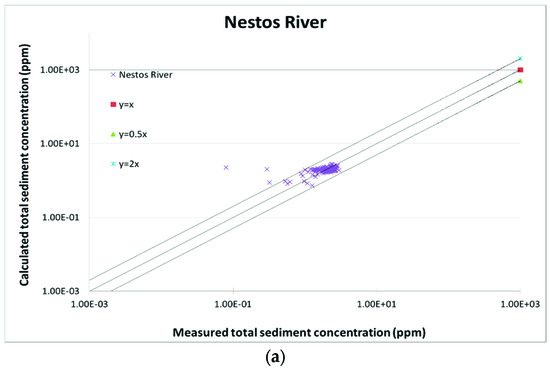
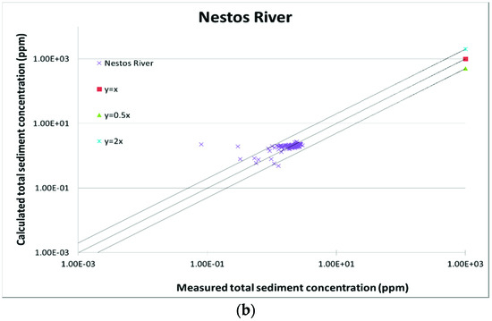
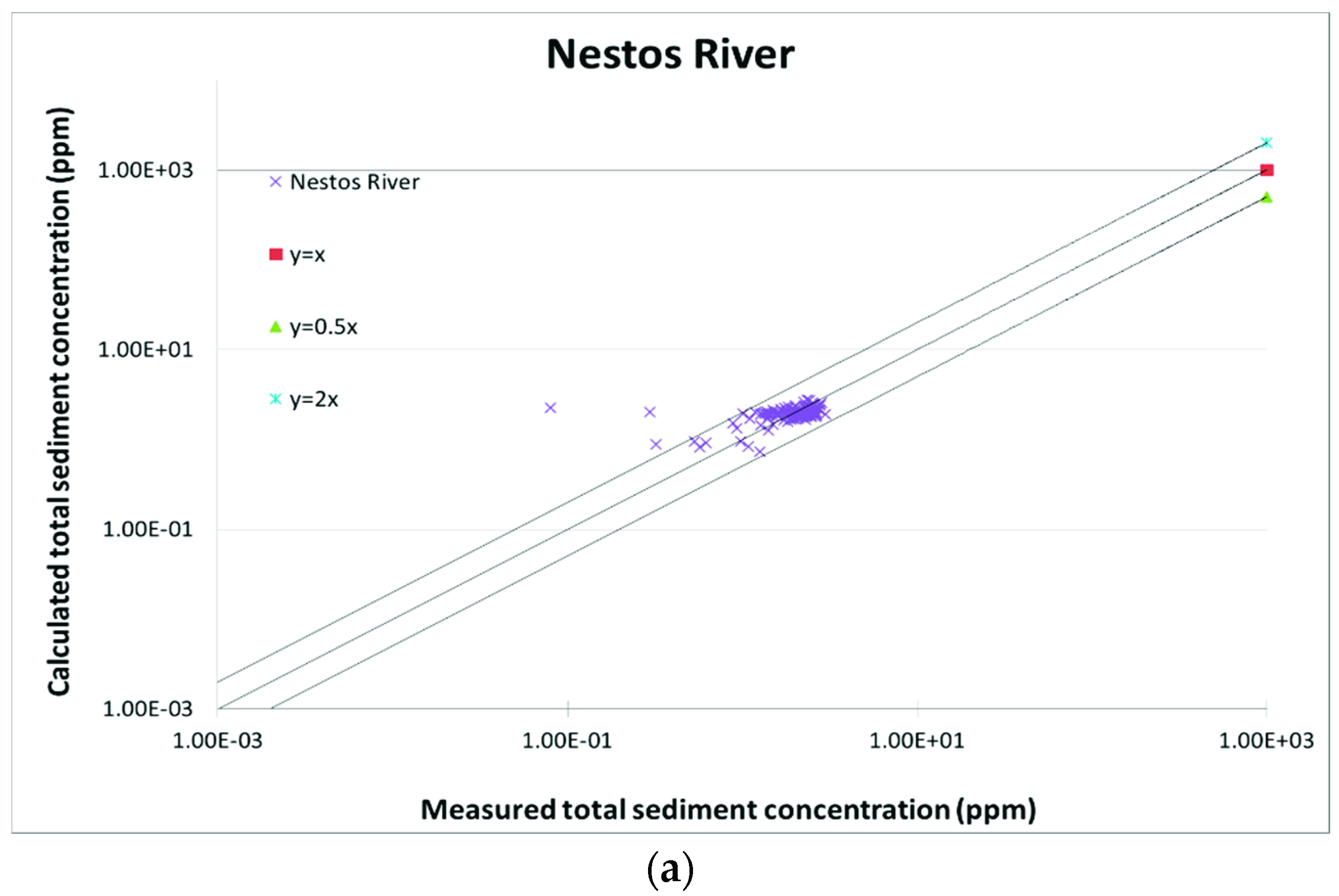
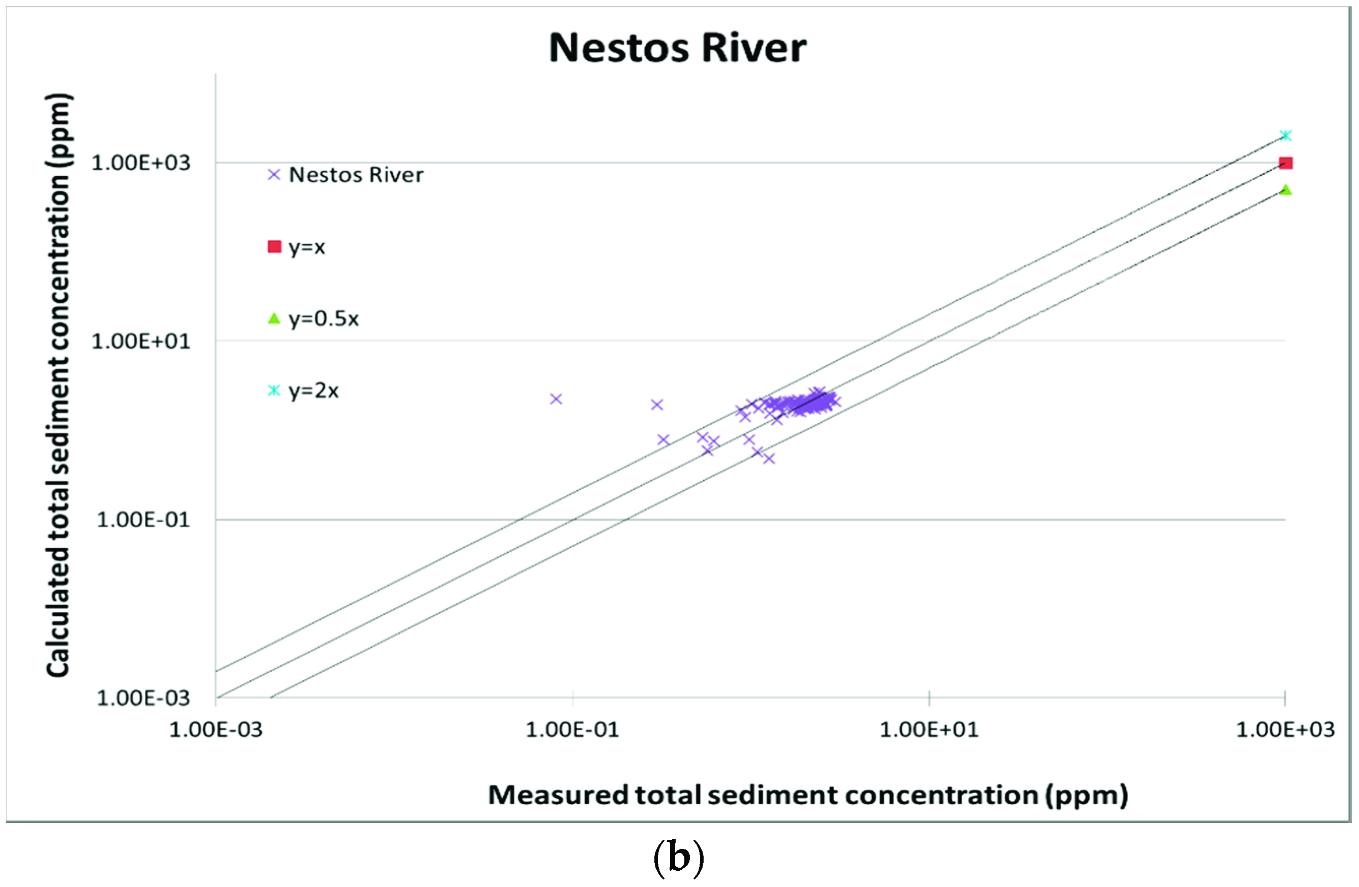
The plot of Figure 1 represents the discrepancy ratio between measured and calculated values of total sediment concentration. At this point, it should be noted that both coordinate axes are in logarithmic scale; therefore, the equations y = x, y = 0.5x and y = 2x are graphically represented by parallel straight lines. Especially the values of the discrepancy ratio, on the basis of the calibrated formulas, are very satisfactory.

Figure 1. Discrepancy ratio plot between measured and calculated values of total sediment concentration by means of: (a) calibrated Yang’s formula (1973) and (b) calibrated Yang’s formula (1979).

7. Discussion—Conclusions

In this paper, an attempt was made to redefine the coefficients of Yang’s formulas based on field measurements data in the Nestos River, between 2005 and 2015. A deviation between the calculated and measured total sediment concentration was observed for this specific case. For the correct application of Yang’s formulas [6,7] to the Nestos River, the calibration of the independent variables’ coefficients was deemed necessary.

As presented above, all statistical criteria of both calibrated Yang’s formulas were improved in comparison to the ones of Yang’s original formulas. More specifically, the RMSE approached zero for the calibrated equations, whilst the MRE displayed a notable decrease. Regarding the NSE, the linear correlation coefficient, r, and the determination coefficient, R², came closer to the optimal value. Particularly, the discrepancy ratio was very near to the optimal value (100%). Overall, the results can be considered satisfactory.

It is noted that the application of Equations (13) and (14) should be bound to the Nestos River.

References

- Kaffas, K.; Hrissanthou, V.; Sevastas, S. Modeling Hydromorphological Processes in a Mountainous Basin Using a Composite Mathematical Model and ArcSWAT. Catena 2018, 162, 108–129. [Google Scholar] [CrossRef] [Scilit]
- Hrissanthou, V.; Tsakiris, G. Sediment Transport in Water Resources: I. Engineering Hydrology; Tsakiris, G., Ed.; Symmetria: Athens, Greece, 1995; pp. 537–577. (In Greek) [Google Scholar]
- Angelis, I.; Metallinos, A.; Hrissanthou, V. Regression analysis between sediment transport rates and stream discharge for the Nestos River, Greece. Glob. NEST J. 2012, 14, 362–370. [Google Scholar]
- Kaffas, K.; Hrissanthou, V. Estimate of continuous sediment graphs in a basin, using a composite mathematical model. Environ. Process. 2015, 2, 361–378. [Google Scholar] [CrossRef] [Scilit]
- Metallinos, A.; Hrissanthou, V. Regression relationships between sediment yield and hydraulic and rainfall characteristics for two basins in northeastern Greece. In Proceedings of the 6th International Symposium on Environmental Hydraulics, Athens, Greece, 1–5 July 2010; Christodoulou, G., Stamou, A., Eds.; Volume 2, pp. 899–904. [Google Scholar]
- Yang, C.T. Incipient motion and sediment transport. J. Hydraul. Div. ASCE 1973, 99, 1679–1704. [Google Scholar] [CrossRef] [Scilit]
- Yang, C.T. Unit stream power equations for total load. J. Hydrol. 1979, 40, 123–138. [Google Scholar] [CrossRef] [Scilit]
- Konstantinopoulou-Pesiou, C.; Sfiris, D. Measurements of Stream Discharge and Sediment Discharge of Nestos River. Diploma Thesis, Department of Civil Engineering, Democritus University of Thrace, Xanthi, Greece, 2013. [Google Scholar]
- Mpenekos, K.; Kassotakis, E. Measurements of Stream Discharge and Sediment Discharge in Nestos River during May and June 2014. Diploma Thesis, Department of Civil Engineering, Democritus University of Thrace, Xanthi, Greece, 2015. [Google Scholar]
- White, W.R.; Milli, H.; Crabbe, A.D. Sediment Transport: An Appraisal of Available Methods. Volume 2: Performance of Theoretical Methods When Applied to Flume and Field Data; INT 119; Hydraulics Research Stations: Wallingford, UK, 1973. [Google Scholar]
- Krause, P.; Boyle, D.P.; Bäse, F. Comparison of different efficiency criteria for hydrological model assessment. Adv. Geosci. 2005, 5, 89–97. [Google Scholar] [CrossRef] [Scilit]
- Nash, J.E.; Sutcliffe, J.V. River flow forecasting through conceptual models, Part I—A discussion of principles. J. Hydrol. 1970, 10, 282–290. [Google Scholar] [CrossRef] [Scilit]
Publisher’s Note: MDPI stays neutral with regard to jurisdictional claims in published maps and institutional affiliations. |
© 2020 by the authors. Licensee MDPI, Basel, Switzerland. This article is an open access article distributed under the terms and conditions of the Creative Commons Attribution (CC BY) license (https://creativecommons.org/licenses/by/4.0/).