Case Study on Improvement Measures for Increasing Accuracy of AI-Based River Water-Level Prediction Model

Abstract

Global warming is recognized as a climate crisis that extends beyond a mere increase in the Earth’s temperature, triggering rapid and widespread climatic changes worldwide. In particular, the frequency and intensity of extreme rainfall events have increased in Korea and the Association of Southeast Asian Nations (ASEAN) region, leading to a significant increase in flood damage. The growing number of large-scale hydrological disasters underscores the urgent need for accurate and rapid flood-forecasting systems that can support disaster preparedness and mitigation. Compared with conventional physics-based forecasting systems, artificial intelligence (AI) models can provide faster predictions using limited observational data. In this study, a river water-level prediction model was constructed using real-time observation data and a long short-term memory (LSTM) algorithm, which is a recurrent neural network-based deep learning approach suitable for hydrological time-series forecasting. A repeated k-fold cross-validation technique was applied to enhance model generalization and prevent overfitting. In addition, water-level differencing was employed to convert nonstationary water-level data into stationary time-series inputs, thereby improving the prediction stability. Water-level observation stations in the Philippines, Indonesia, and the Republic of Korea were selected as study sites, and the model performance was evaluated at each location. The differenced LSTM model achieved a root mean square error of 0.13 m, coefficient of determination (R²) of 0.866, Nash–Sutcliffe efficiency (NSE) of 0.844, and Kling–Gupta efficiency of 0.893, thus outperforming the non-differenced baseline by approximately 17%. The repeated k-fold validation approach was particularly effective when the training data period was short or the number of input variables was limited. These results confirm that ensuring temporal stationarity and applying repeated cross-validation can significantly enhance the predictive accuracy of real-time flood forecasting. The proposed framework exhibits strong potential for implementation in regional early warning systems across data-limited flood-prone areas in the ASEAN region. Ongoing studies that apply and verify this approach in diverse hydrological contexts are expected to further improve and expand AI-based flood prediction models.

1. Introduction

Abnormal weather conditions worldwide are a direct consequence of accelerating global warming. These phenomena are no longer regarded as mere abnormal weather patterns but are now recognized as indicators of a global climate crisis. The “heat dome” phenomenon, which is characterized by high pressure trapping hot air, can cause prolonged heat waves with temperatures approaching 40 °C. Moreover, global warming intensifies atmospheric moisture retention, leading to more frequent and severe rainfall events. In particular, flood damage caused by extreme rainfall is one of the most destructive natural disasters, resulting in both high casualties and extensive socioeconomic losses. According to the World Resources Institute, the number of people directly or indirectly affected by floods is expected to double between 2010 and 2030, reaching approximately 132 million [1]. The scale and frequency of flood hazards along coastlines and rivers are therefore projected to increase substantially, a concerning trend that highlights the need for accurate and rapid advanced flood forecasting to mitigate potential damage.

Korea and the Association of Southeast Asian Nations (ASEAN) are among the regions that are most vulnerable to climate-driven hydrological changes. In Korea, localized flash floods occur frequently, rainfall intensity continues to increase, and the number of short-duration high-impact flood events has steadily increased. Numerous ASEAN countries are islands or coastal nations located near the equator, and are constantly exposed to heavy rainfall and typhoons. For instance, Indonesia, which traditionally experiences distinct dry and rainy seasons, has recently suffered severe flooding, even during the dry season, owing to abnormal rainfall. In addition, excessive groundwater extraction has caused serious land subsidence, making numerous areas of Jakarta, already below sea level, the fastest sinking areas in the world. Consequently, the risk of inundation is increasing annually. The Philippines receives rainfall frequently because of its tropical climate, causing floods and landslides throughout the nation, particularly during the rainy season. Moreover, it experiences an extremely high typhoon frequency. An average of 20 typhoons occur annually in the Philippines. Typhoons are accompanied by strong winds and heavy rainfall that cause damage to life and property, rendering large populations highly vulnerable to flood damage.

Accurate and rapid flood prediction systems have become critical for mitigating the growing threat of flood disasters. The most widely studied flood forecasting methods can be broadly categorized into three groups: (1) physical models, based on mathematical and physical equations. Although they are the most reliable, they require extensive calibration and high computational costs, thus limiting their use in real-time forecasting [2,3]; (2) statistical models, which analyze previous flood data to predict future events. These models do not simulate physical processes, but instead predict floods based on statistical relationships and probabilities [4,5]. (3) Data-driven models (machine learning (ML) models) have recently garnered significant attention. These models employ artificial intelligence (AI) algorithms to recognize complex patterns and relationships in previous datasets. They leverage correlations within the data instead of physical relationships. Although learning requires significant computational costs, predictions do not, resulting in extremely fast prediction speeds, which makes them promising for real-time forecasting [6,7].

Among the numerous AI algorithms, the long short-term memory (LSTM) algorithm of recurrent neural networks (RNNs) has been widely applied to time-series prediction. Le et al. predicted the discharge in the Da River Basin in Vietnam using an LSTM algorithm [8,9,10]. The discharge for days 1, 2, and 3 was predicted based on daily discharge and rainfall, and the accuracy was evaluated based on the Nash–Sutcliffe efficiency (NSE) [11]. Ding et al. proposed an interpretable spatiotemporal attention (STA) LSTM model that offers better flood-prediction performance and interpretability than the vanilla LSTM, and achieved higher accuracy than the vanilla LSTM, temporal attention, and spatial attention [12]. Fang et al. applied the LSTM algorithm to flood-vulnerability prediction, and the improved local spatial sequential-LSTM technique performed well in processing the spatial relationship of floods. Generated flood vulnerability maps can be used as basic information by decision makers [13]. Kim et al. developed an AI-based river flood-prediction model combined with an observation station, providing independent self-warning as an alternative to a centrally controlled flood-forecast system [14]. The flood-prediction model based on the LSTM algorithm can predict for up to 6 h, and in the case of mountainous rivers as the study area, it was predicted to enable flood forecasting within 1 h. Zhang et al. compared the water-level prediction results of the LSTM algorithm with those of the convolutional LSTM, STA-LSTM, gated recurrent unit (GRU), convolutional neural network (CNN)-GRU, and STA-GRU and indicated that the STA-GRU model achieved the best performance [15]. Oddo et al. proposed a model that predicts flash floods using a deep convolutional LSTM. This model reflects spatiotemporal characteristics by utilizing multimodal input data that combine rainfall radar and ground observation data [16]. Fuente et al. showed that the LSTM architecture is structurally similar to that of the hydrological reservoir model, proposed a new HydroLSTM model that is concise and more interpretable, and analyzed its computational efficiency compared with that of LSTM [17]. Malik et al. proposed a time distribution (TD)-CNN-LSTM, which is a hybrid deep-learning (DL) framework based on a TD layer, CNN, and LSTM network. The results demonstrated that the proposed model performed well in predicting the start time of a flood and the time of maximum flood occurrence [18]. As previously discussed, most LSTM-based research has focused on improving the spatiotemporal structure of the algorithm, with few studies addressing the problems caused by overfitting and nonstationarity in limited hydrological datasets. Therefore, despite these advancements in AI algorithms, overfitting and nonstationarity in hydrological data remain critical challenges that degrade model generalization. Consequently, this study examined the contribution of repeated k-fold cross-validation (to reduce overfitting) and water-level differencing (to ensure time-series stationarity) toward improving flood forecast accuracy by performing flood forecasts at major water-level stations in the Philippines, Indonesia, and South Korea. Accordingly, this study aimed to develop an LSTM-based flood prediction model capable of real-time application across diverse regions in Asia and evaluate the generalization performance of the model under different temporal and hydrological conditions.

2. Basic Theory

In this study, a river water-level prediction model was constructed using a DL approach based on the LSTM algorithm. The model utilized real-time observation data obtained from water-level stations located in the Philippines, Indonesia, and the Republic of Korea. The AI learning/inference algorithms, cross-validation methodology, and normal data transformation techniques used in this study were as follows.

2.1. LSTM

The AI-based river water-level prediction model developed in this study uses real-time observation data as input data and predicts the water level every 10 min for up to 6 h. The minimum forecast was 10 min because the new observation data were updated every 10 min, and the maximum forecast was 6 h to ensure sufficient time to recognize and respond to flood risks. LSTM is a type of RNN designed to capture long-term dependencies in sequential data through a gating mechanism that regulates information flow [19]. Therefore, the LSTM was selected as the primary model in this study because it effectively captures the nonlinear and long-term temporal relationships inherent in hydrological processes, such as rainfall–runoff and river stage variations. The four hidden layers interact with each other to continuously transmit information to the next stage without significant changes [20] (Figure 1).

Figure 1. Schematics of RNN and LSTM [20].

2.2. Repeated k-Fold Cross-Validation

When training an ML algorithm, overfitting can easily occur if the model is trained using fixed training and test data. To prevent overfitting, cross-validation was performed and the training and validation data were organized into several separate sets to train the model. k-fold cross validation is the most widely used cross-validation technique. However, standard k-fold validation can overfit the first-fold learned owing to look-ahead bias, thereby hindering smooth learning in subsequent folds.

Therefore, the repeated k-fold method has been proposed, which moves to the next fold before fold learning is fully completed, and repeats this process to ensure even training across all folds. Wong and Yeh reported that the accuracy estimates obtained from various repetitions of the k-fold generally exhibited high correlations that increased with the number of repetitions [21]. As suggested by Marcot and Hanea, the error decreased as the K value increased; however, convergence was observed at a K value of 10 but a K value of 5 was reported as sufficient for samples exceeding 5000 [22]. Because the data used in this study comprised at least 70,000 samples, the K value was set to 5 and repeated five times. Finally, the model with the lowest loss of validation when training each fold was selected as the best model and used for prediction. The procedure for calculating repeated k-folds is presented in Figure 2.

Figure 2. Diagram showing procedure for calculating repeated k-folds (■: Training data, ■: Test data).

2.3. Converting to Stationary Time-Series Data

Time-series data are classified into stationary and nonstationary. Because of the mean, variance, and autocorrelation of the nonstationary time series with time change, one cannot easily predict and analyze the time series. Additionally, because most time-series models assume stationarity, nonstationary time series must be converted into stationary time series for time-series prediction. Converting nonstationary time series into stationary time series renders data analysis and prediction more accurate and increases model reliability [23]. Hydrological data such as river water levels are typically nonstationary, implying that their statistical properties change over time. Nonstationarity can cause unstable learning and poor generalization in DL models.

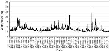
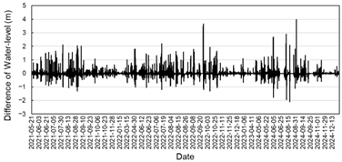
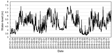
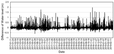
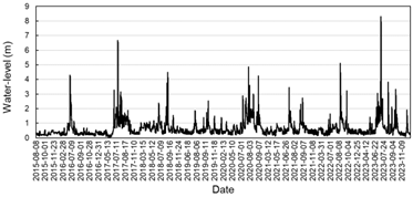
An augmented Dickey–Fuller (ADF) test was applied to statistically verify the nonstationarity of the data. The results confirmed that the maximum flood events in each country were nonstationary (p > 0.05). After determining the difference in water level (ΔH_t = H_t − H_t−1), the data were converted to stationary data (p > 0.05) (Table 1, Figure 3).

Table 1. Results of ADF test for water-level observation data of each country.

Target Station	p-Value
	Original	Water-Level Differencing
San Mateo-1 (Philippines)	0.179 (>0.05, Nonstationary)	0.003 (<0.05, Stationary)
Dayeuh Kolot (Indonesia)	0.222 (>0.05, Nonstationary)	7.783 × 10−7 (<0.05, Stationary)
Goesangun (Mokdogyo) (Republic of Korea)	0.093 (>0.05, Nonstationary)	0.003 (<0.05, Stationary)

Figure 3. Stationary evaluation of water-level differencing convert.

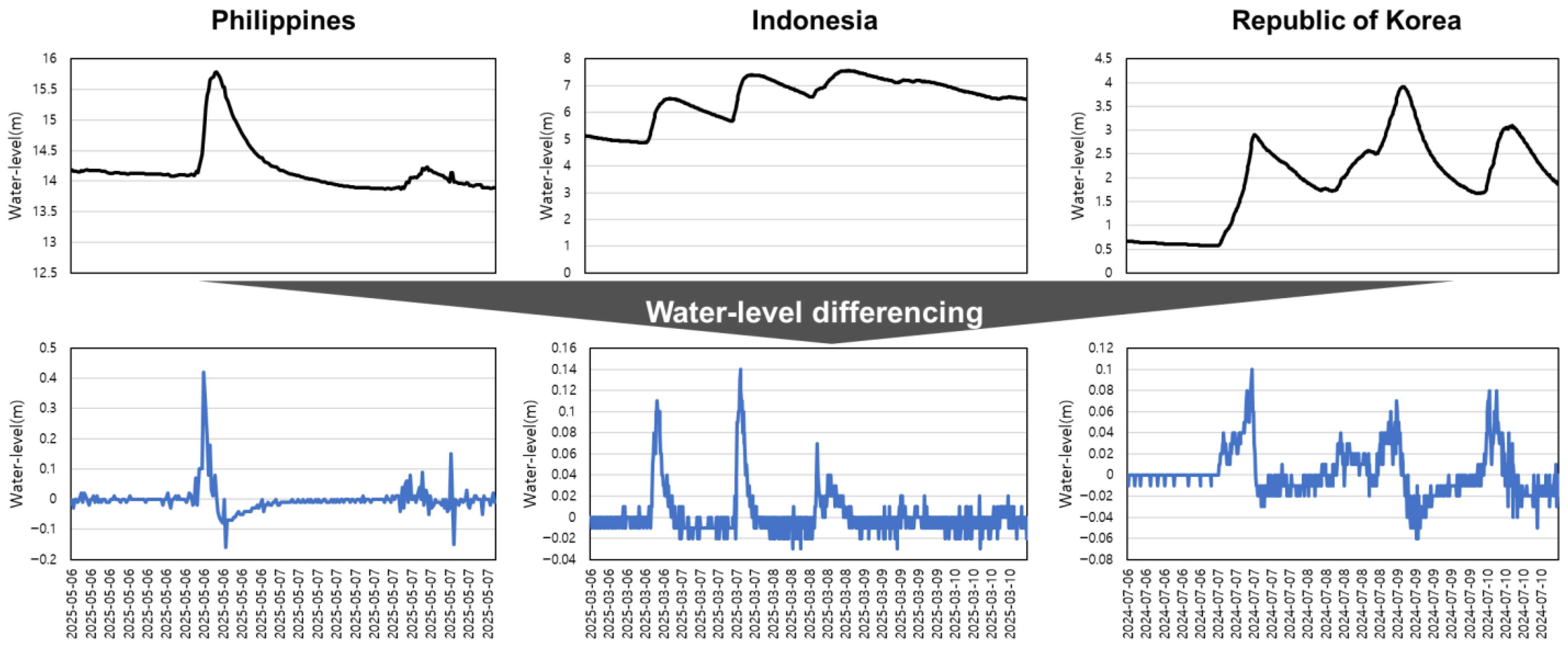
The main methods for converting nonstationary time series into stationary time series include first differences, seasonal differences, and log transformations. In this study, a method was used to differentiate the predicted values from the observed values for each prediction lead-time. The conversion equation is Equation (1) below, and the procedure is illustrated in Figure 4:

$$d_{t+Leadtime}=H_{t+Leadtime}-H_t$$

(1)

where $d_t$ denotes the difference between the predicted and observed values, $H_t$ denotes the water level at time $t$, $t$ denotes the observation time, and $Leadtime$ denotes the prediction lead time.

Figure 4. Calculation of difference between predicted water levels by lead time.

3. Methodology

This study targeted water level stations in the Philippines, Indonesia, and South Korea. The target stations were surrounded by reference stations where observational data could be used. After the decision to conduct the study, three steps were sequentially conducted for each country: (1) data collection and preprocessing, (2) model construction and validation, and (3) performance evaluation.

3.1. Study Area

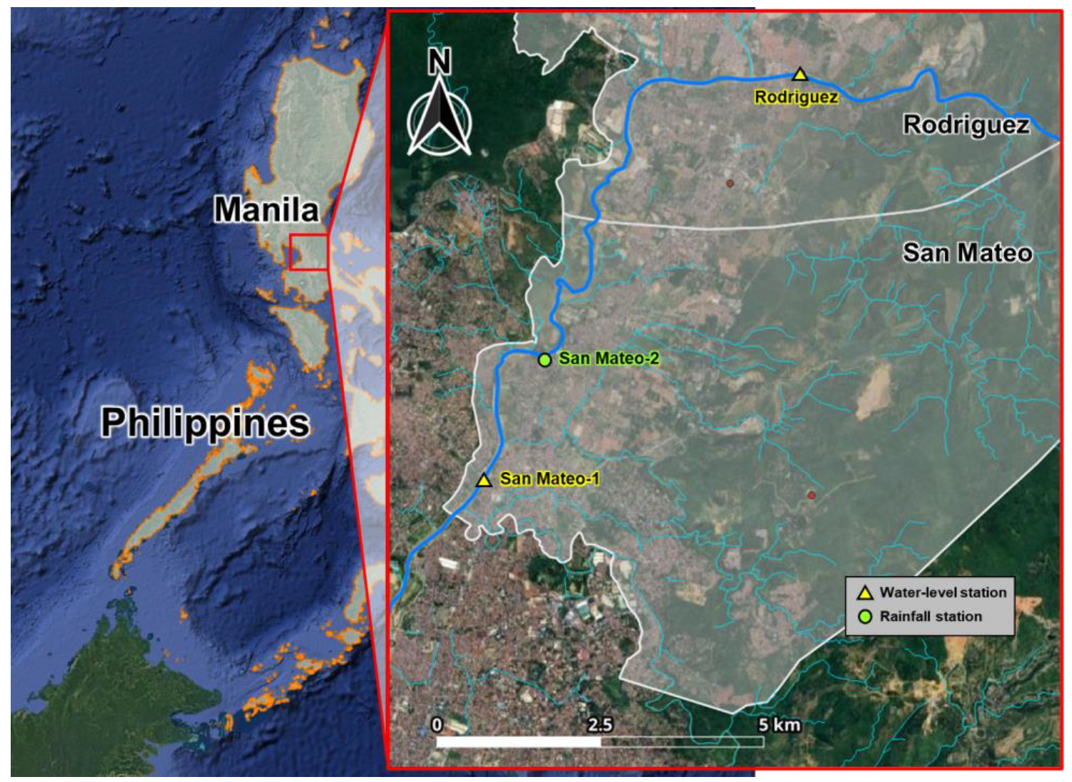
The Marikina River in the Philippines flows east of metropolitan Manila. It originates from the Rizal and Rodriquez areas and joins the Pasig River. The San Mateo-1 water-level observation station is located downstream of the San Mateo area, which frequently experiences flood damage owing to river overflow (Figure 5).

Figure 5. Location map of San Mateo-1 and reference stations in the Philippines.

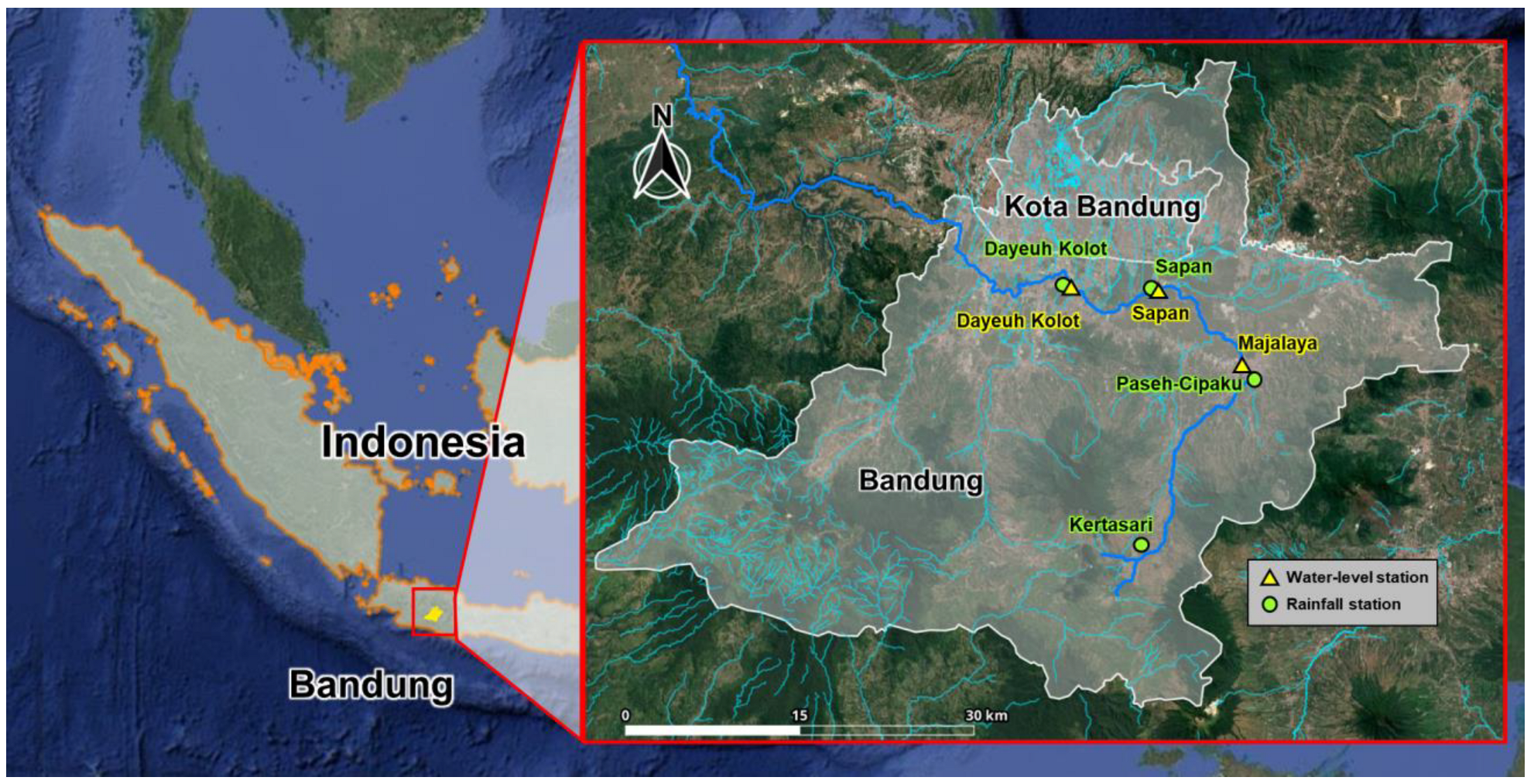
The Citarum River in West Java, Indonesia, supplies 80% of Jakarta’s domestic water and is an important river that provides water resources and hydroelectric power to 25 million metropolitan residents. The upstream part of the Citarum River Basin is mountainous and steep, whereas the downstream part is a lowland area where flood damage occurs frequently during the rainy season. The Dayeuh Kolot water-level station is located south of Kota Bandung, and the surrounding areas are flatlands with minimal elevation changes, implying that it experiences extensive flooding when rivers overflow (Figure 6).

Figure 6. Location map of Dayeuh Kolot and reference stations in Indonesia.

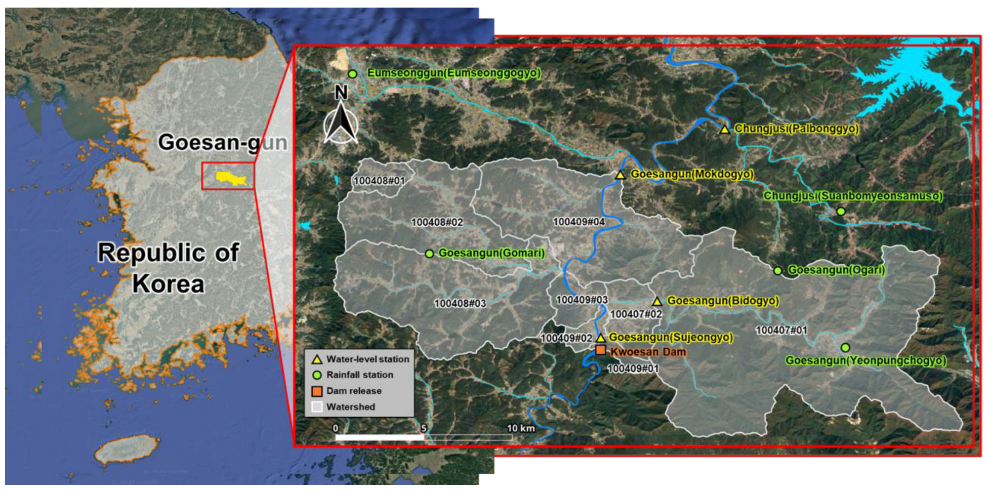
Goesan-gun is located in central Korea, through which the Dalcheon River, a tributary of the Han River, the largest river in the country, flows. Kwoesam Dam is located upstream of the Goesangun (Mokdogyo) water level station. The water level of the Dalcheon River is significantly affected by the amount of dam discharge, and four tributaries flow between the Goesangun (Mokdogyo) station and the dam. The basin is primarily mountainous (Figure 7).

Figure 7. Location map of Goesangun (Mokdogyo) and reference stations in Republic of Korea.

The San Mateo-1 target station comprises the Rodriquez water-level station and San Mateo-2 rainfall station upstream. Only few reference observation stations are present in the surrounding areas. The Dayeuh Kolot target station comprises the Majalaya and Sapan water-level stations upstream, which can be input with various types of data, such as the Kertasari rainfall station located in the mountainous area upstream, the Paseh–Cipaku rainfall station located in the hilly area, and the Sapan and Dayeuh Kolot rainfall stations located in the urban area. The Goesangun (Mokdogyo) target station comprises the Kwoesan Dam located upstream, and three reference water level stations are available upstream and downstream. The upstream basin was classified into nine subbasins, and the average rainfall for each subbasin was calculated using the Thiessen network and used as training data. Five rainfall observation stations in the surrounding area were used as input data (Table 2).

Table 2. Details of reference stations by target stations.

Target Station	Reference Station
	Type (Number)	Name
San Mateo-1 (Philippines)	Water level (1)	Rodriguez
	Rainfall (1)	San Mateo-2
Dayeuh Kolot (Indonesia)	Water level (2)	Majalaya, Sapan
	Rainfall (4)	Kertasari, Paseh-Cipaku, Sapan, Dayeuh Kolot
Goesangun (Mokdogyo) (Republic of Korea)	Water level (3)	Goesangun (Sujeongyo), Goesangun (Bidogyo), Chungjusi (Palbonggyo)
	Rainfall (5)	Goesangun (Yeonpungchogyo), Goesangun (Ogari), Chungjusi (Suanbomyeonsamuso), Goesangun (Gomari), Eumseonggun (Eumseonggogyo)
	Dam release (1)	Kwoesan Dam
	Average rainfall of watershed (9)	100407#01, 100407#02, 100408#01, 100408#02, 100408#03, 100409#01, 100409#02, 100409#03, 100409#04

3.2. Data Preprocessing and Dataset

3.2.1. Observation Data Acquisition and Preprocessing

The hydrological data of the three countries were obtained from different periods depending on their respective situations and observation conditions. In the case of the Philippines, data were obtained from 2018, whereas some reference observation stations provided observational data from 2021; therefore, the training period was limited to 2021–2025. In the case of Indonesia, observational data were obtained from 2017; however, observational data from 2019 to 2024, which was the construction period of the flood prediction system, were not available and were outliers, thus rendering their usage challenging. In the case of Korea, because flood season data have not yet been obtained for 2025, data until October 2024 (i.e., the flood season) were used for the analysis (Table 3).

Table 3. Observation period and number of data points.

Target Station	Period of Observation Data	Number of Data Points	Remarks
San Mateo-1 (Philippines)	21 May 2021 02:00–19 May 2025 11:10	77,550	Missing data 2018–2021
Dayeuh Kolot (Indonesia)	11 January 2017 09:50–30 April 2025 23:50	73,642	Missing data 2019–2024
Goesangun (Mokdogyo) (Republic of Korea)	8 August 2015 03:30–30 October 2024 23:50	156,949

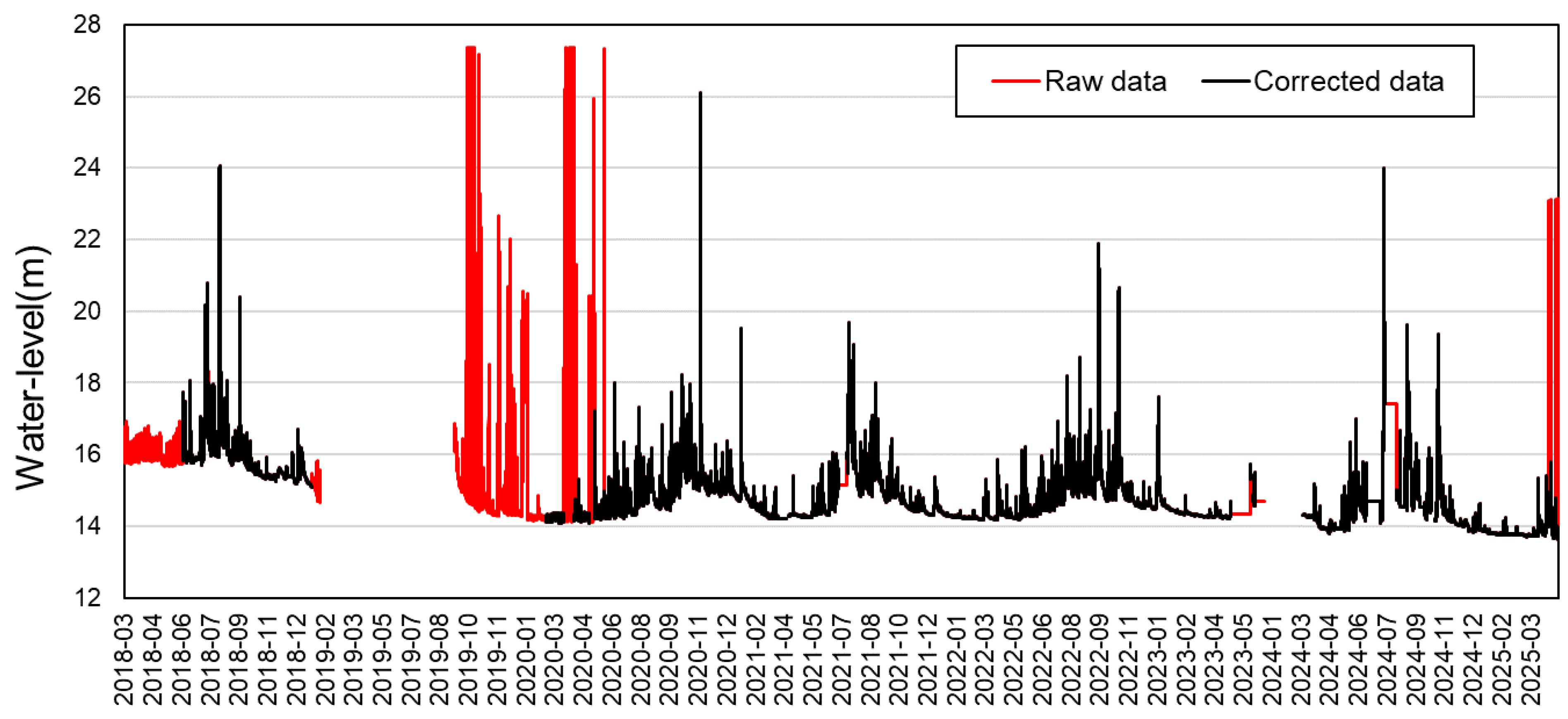
Each observation dataset included missing data and outliers; thus, the missing and outlier data were corrected for AI training. For the water-level data, linear interpolation was performed for missing data within 3 h, and missing data for 3 h or more were excluded from the training. For rainfall data, missing and negative values were corrected to zero. Outlier data were plotted on a graph, and intervals and values for which stable observational data were not obtained were excluded. If no rainfall occurred at all reference rainfall stations for 12 h before and after the corresponding time, then it was excluded as a no-rain period unrelated to flooding to increase the training efficiency (Figure 8). When creating a dataset with a size equal to the sequence length, the data were processed to skip the sequence length after the no-rain period, thereby preventing the addition of discontinuous periods owing to the deletion of the no-rain period.

Figure 8. Preprocessing of water-level data in San Mateo-1 (Philippines) (example).

3.2.2. Data Composition

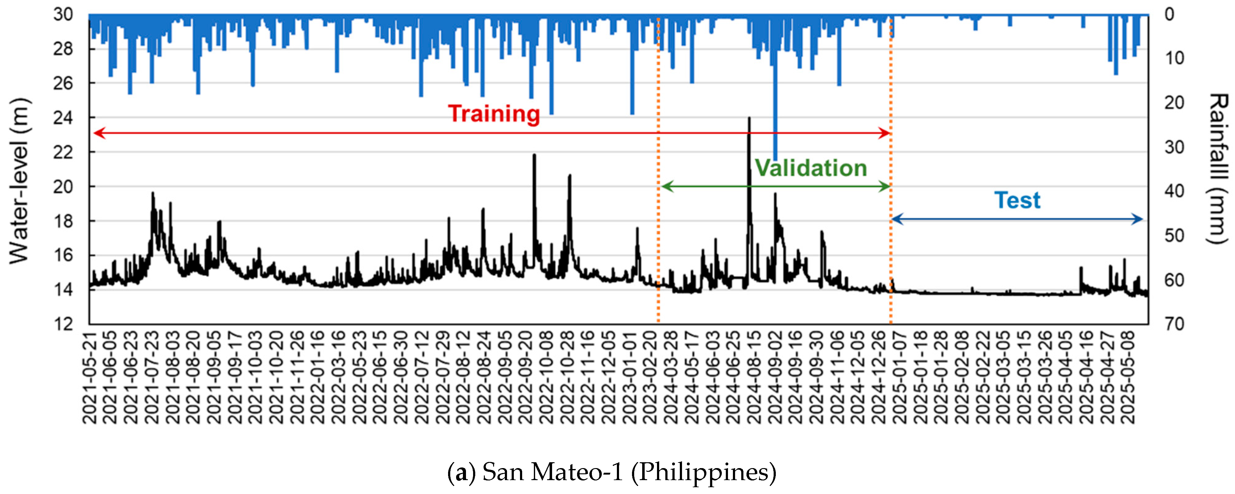
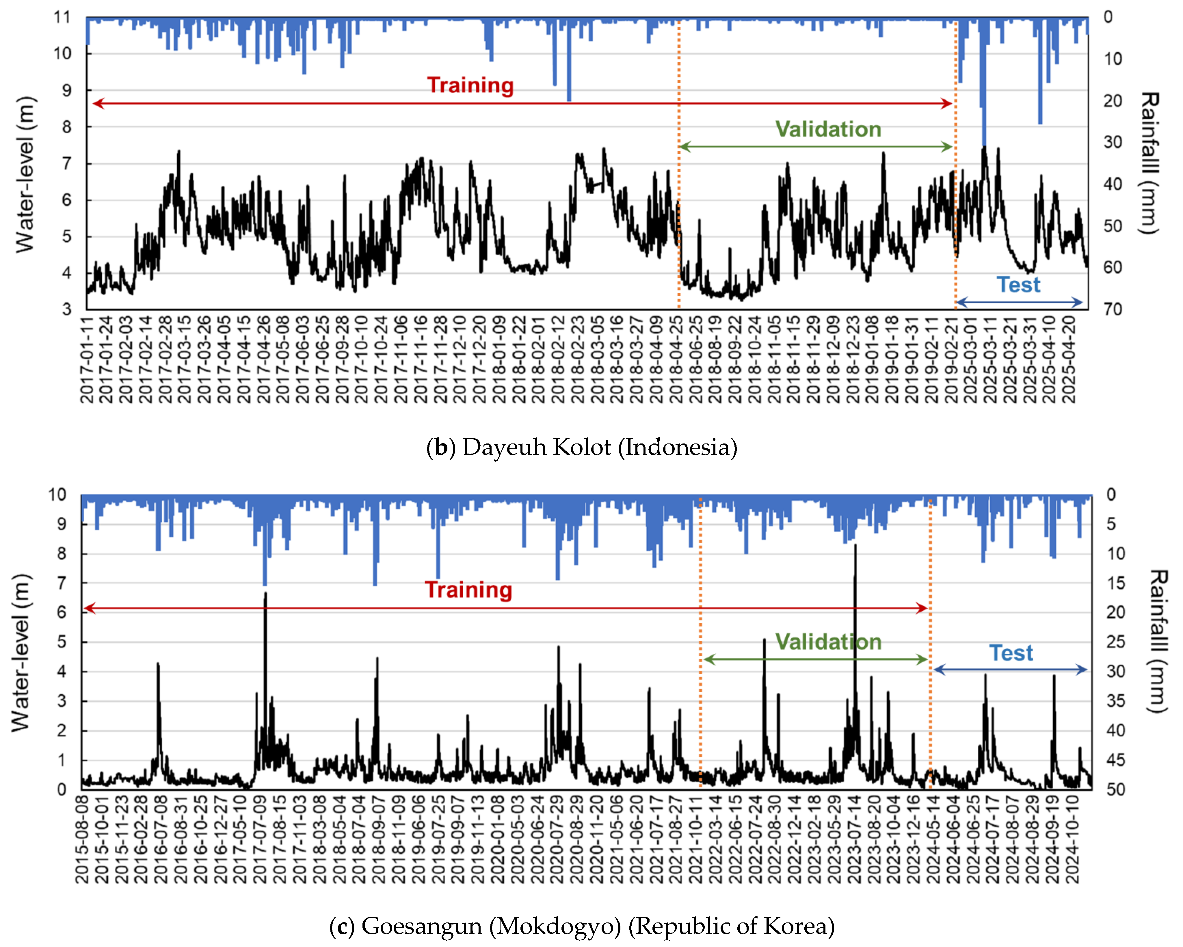
The AI prediction model dataset comprised three components. The training dataset was used for training, validation dataset was used for validation during training, and test dataset was used to evaluate the performance of the trained model. For the Philippines and Indonesia, 2025 data points were used as the test dataset, and for Korea, 2024 data points were used as the test dataset. All data points before the test dataset were used for training, and 30% of each dataset was used as the validation dataset. The dataset composition for each model is shown in Figure 9.

Figure 9. Dataset composition for AI-prediction model learning) (––: water-level, ––: rainfall).

3.2.3. Generating Water-Level Difference

Water-level data are nonstationary time series, and predicting the time series is challenging. Therefore, to ensure prediction accuracy, data for the differences in water level were created and converted into a stationary time series. The conversion was performed for all lead times, and Table 4 summarizes the differences in the water levels for a lead time of 180 min.

Table 4. Converting water level to water-level difference.

Target Station	Water Level	Difference in Water Level (After 180 min)
San Mateo-1 (Philippines)
Dayeuh Kolot (Indonesia)
Goesangun (Mokdogyo) (Republic of Korea)

3.3. Model Creation

3.3.1. Prediction-Model Calculation Procedure

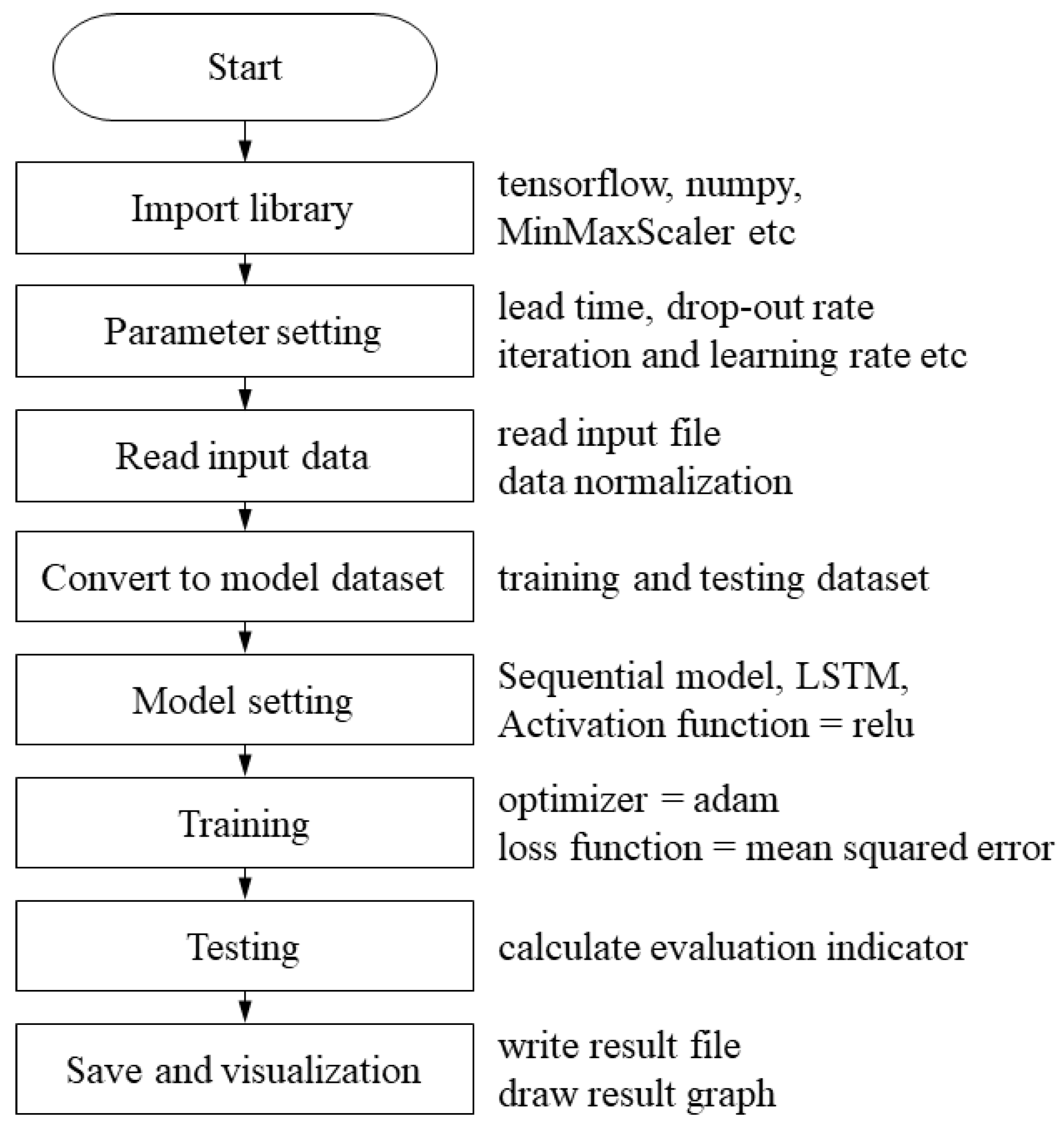
The computational structure of the LSTM constructed using TensorFlow is shown in Figure 10. First, the libraries used in the model were loaded, the input data were read, and the training parameters were set. The data were normalized using MinMaxScaler, and the input data were converted into training, validation, and test datasets. Subsequently, the hyperparameters of the LSTM model were set, model training was performed, and the results were saved. Validation was performed using a trained model. The prediction (test process) was performed using the test dataset, and a prediction-accuracy evaluation index was calculated. Finally, a program was developed to save the validation and prediction results as a file and display them as a graph.

Figure 10. Calculation procedure for AI prediction model.

3.3.2. Model Parameter Setting

When creating a model using AI, the appropriate parameters must be selected for training. The efficiency and accuracy of training are determined by the parameter set, which must be set depending on the training type. A nonlinear rectified linear unit (ReLU) function was used as the activation function for the LSTM applied in this study. Adam was used as the optimizer and the mean squared error was used as the loss function. The hidden layer was designed with three layers to achieve a DL ANN structure. Because the arrival time of a river considered in flood forecasting is generally 3–4 h, the sequence length was set to 24 such that rainfall occurrence was sufficiently reflected in the water-level change. This implies that the input data used were from the observation data obtained 4 h prior. The other training parameters used in the models are listed in Table 5.

Table 5. Training-model parameters.

Parameter	Value	Parameter	Value
Activation Function	ReLU	Optimization algorithm	Adam Optimizer
Loss Function	Mean Squared Error	Hidden layer	Three layers (32, 64, 32)
Sequence_length	24	Learning_rate	0.0001
Epochs	300	Batch_size	48

4. Study Results

4.1. Validation Results of Trained Model

After completion of model training using the training dataset, the validation dataset was used to verify the suitability of each station and lead time. The NSE coefficient, the most widely used index for evaluating the prediction technology of hydrological models, was used as an indicator for suitability validation [24]. Equation (2) was used to calculate the NSE. The suitability grade of the NSE values for the time-series prediction was classified based on the lead time using the grade criteria suggested by Moriasi et al. [25] (Table 6).

Table 6. Ranges of statistics by grade [25].

Grade	Very Good	Good	Satisfactory	Not Satisfactory
NSE	NSE ≥ 0.80	0.80 > NSE ≥ 0.70	0.70 > NSE ≥ 0.50	0.50 > NSE

The training validation results for each target station had a maximum of 1.0, and a minimum of 0.962 for all lead times. Based on the criteria suggested by Moriasi et al. [25], they indicated “very good” levels (Table 7).

$$NSE=1-{\displaystyle \frac{{\sum }_{i=1}^n{(O_i-P_i)}^2}{{\sum }_{i=1}^n{(O_i-\overline{O})}^2}}$$

(2)

Here, $O$ denotes the observed data, $P$ denotes the predicted data, and $\overline{O}$ denotes the average of the observed data.

Table 7. Validation results for trained model.

Target Station	Very Good	Lead Time (min)
		30	60	120	180	240	300	360
San Mateo-1 (Philippines)	Basic	0.995	0.994	0.99	0.984	0.979	0.975	0.971
	Repeated k-fold	0.997	0.996	0.995	0.992	0.99	0.99	0.987
	Basic_diff	0.997	0.995	0.991	0.984	0.979	0.974	0.969
Dayeuh Kolot (Indonesia)	Basic	0.999	0.998	0.994	0.989	0.983	0.974	0.962
	Repeated k-fold	0.999	0.999	0.998	0.997	0.996	0.995	0.991
	Basic_diff	0.999	0.998	0.995	0.99	0.984	0.975	0.963
Goesangun(Mokdogyo) (Republic of Korea)	Basic	0.999	0.998	0.997	0.995	0.992	0.987	0.974
	Repeated k-fold	0.999	0.999	0.999	0.998	0.998	0.997	0.996
	Basic_diff	1.000	0.999	0.998	0.995	0.991	0.985	0.977

Note—██: Very good, ██: Good, ██: Satisfactory, ██: Not satisfactory.

4.2. Prediction Results of Trained Model

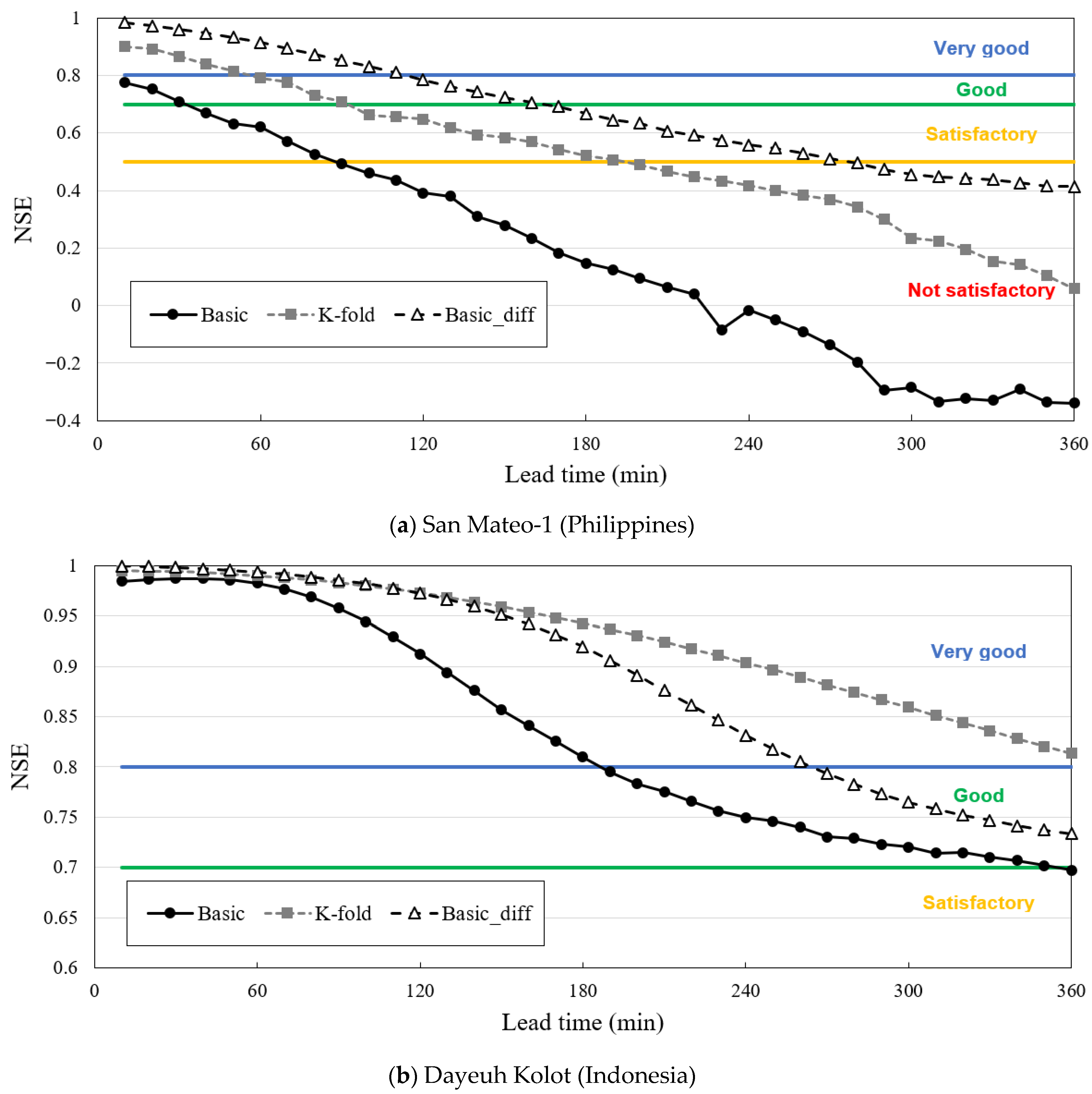
The water level was predicted by inputting a test dataset using a trained model. The test dataset was separated from the training dataset under the same conditions as the actual prediction model. The NSE values for each target station and predicted lead times are listed in Table 8.

Table 8. Prediction results for trained model.

Target Station	Very Good	Lead Time (min)
		30	60	120	180	240	300	360
San Mateo-1 (Philippines)	Basic	0.709	0.621	0.391	0.148	−0.016	−0.285	−0.339
	Repeated k-fold	0.867	0.791	0.648	0.522	0.417	0.233	0.059
	Basic_diff	0.960	0.914	0.784	0.667	0.558	0.455	0.414
Dayeuh Kolot (Indonesia)	Basic	0.987	0.982	0.912	0.810	0.750	0.720	0.697
	Repeated k-fold	0.994	0.990	0.973	0.942	0.904	0.859	0.813
	Basic_diff	0.998	0.994	0.973	0.919	0.832	0.765	0.734
Goesangun(Mokdogyo) (Republic of Korea)	Basic	0.998	0.997	0.991	0.980	0.963	0.941	0.913
	Repeated k-fold	0.997	0.995	0.989	0.976	0.956	0.931	0.902
	Basic_diff	0.999	0.997	0.991	0.980	0.963	0.940	0.913

Note—██: Very good, ██: Good, ██: Satisfactory, ██: Not satisfactory.

For the San Mateo-1 target station in the Philippines, the NSE value for the basic model was 0.148 (good) for water-level prediction after 180 min. Meanwhile, the repeated k-fold model was 0.522 (satisfactory), and the Basic_diff model was 0.667 (satisfactory). Although the repeated k-fold model and conversion of the stationary time series improved the overall model suitability, securing an accuracy level that could be used for real-time prediction was challenging. This is because only one upstream water level was available and only one rainfall station could be used as a reference station, which was insufficient for training the correlation between the input variables and the predicted values (Figure 11a).

Figure 11. Results of test process for trained model.

For the Dayeuh Kolot target station in Indonesia, the NSE value for the basic model was 0.810 (very good) for water level prediction after 180 min. Meanwhile, the repeated k-fold model indicated 0.942 (very good) and the Basic_diff model indicated 0.919 (very good). The Dayeuh Kolot target station had the smallest amount of training data; therefore, the effect of repeated k-fold cross-validation was assumed to be prominent. Repeated k-fold cross-validation is useful when the number of data points is insufficient. Owing to the sufficient water levels and rainfall stations upstream of the target point for reference, it may be assumed that the trained model can be sufficiently utilized for real-time prediction (Figure 11b).

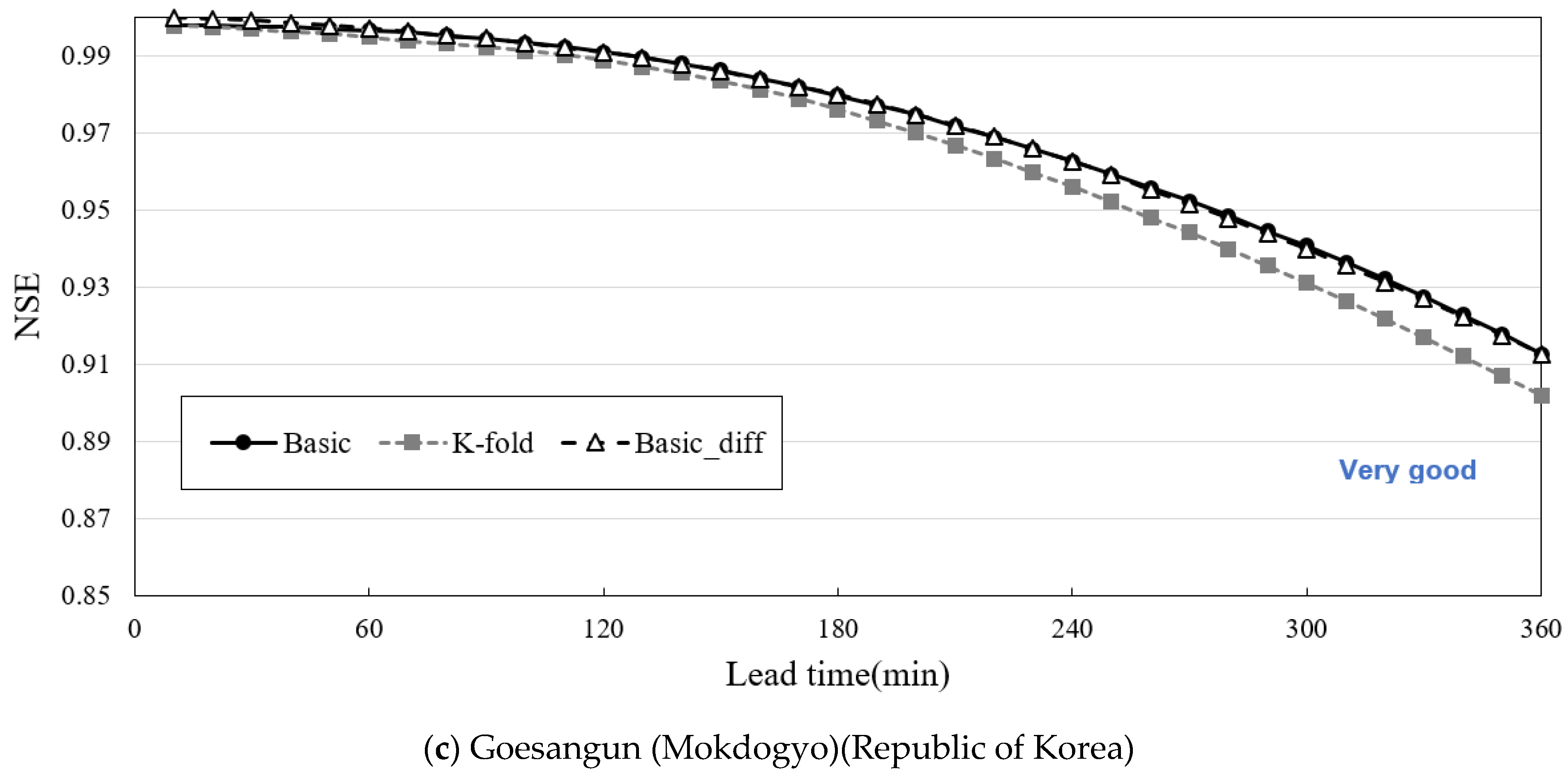
For the Goesangun (Mokdogyo) target station in the Republic of Korea, the NSE value for the basic model was 0.980 (very good) for water level prediction after 180 min. Meanwhile, the repeated k-fold model was 0.976 (very good), and the Basic_diff model was 0.980 (very good). The Goesangun (Mokdogyo) target station secured more than 10 y of data, and numerous reference stations were distributed in the upstream and downstream areas. Therefore, it was considered sufficient for training the correlation between each station. In particular, the release amount of the dam located upstream can be used as training data; therefore, the effect of dam release on the water-level change can be considered. However, the effect of repeated k-fold cross-validation was marginal when a sufficient amount of training data was secured. Even when the predicted values were converted into a stationary time series, the overall suitability did not significantly differ from that of the basic model (Figure 11c).

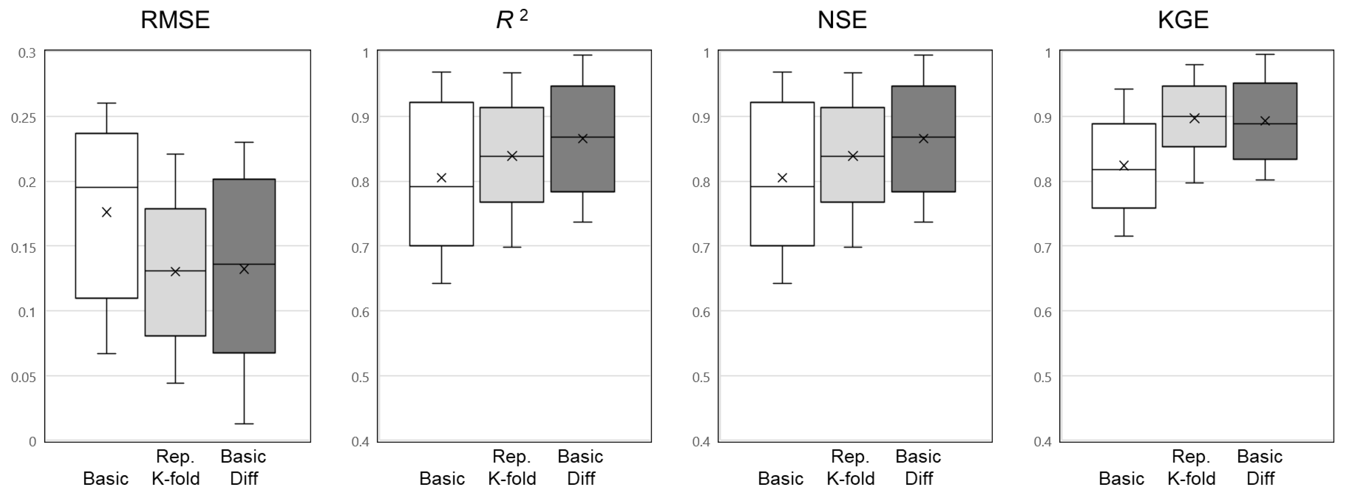
Additionally, four quantitative metrics were used to compare the model performance across various metrics: root mean square error (RMSE, a measure of the average magnitude of prediction errors; lower values indicate better performance), coefficient of determination (R², a measure of how well predictions explain observed variance; 1 indicates perfect prediction), NSE (a measure of predictive accuracy; 1 indicates perfect prediction), and Kling–Gupta efficiency (KGE, a combined measure of correlation, bias, and variability agreement; 1 indicates perfect prediction). The calculation formulas for each metric are given in Equations (3)–(5).

$$RMSE=\sqrt{{\displaystyle \frac{1}{n}} \sum _{i=1}^n{\left(O_i-P_i\right)}^2}$$

(3)

$$R^2={\left[{\displaystyle \frac{{\sum }_{i=1}^n(O_i-\overline{O})(P_i-\overline{P})}{\sqrt{{\sum }_{i=1}^n{(O_i-\overline{O})}^2}\sqrt{{\sum }_{i=1}^n{(P_i-\overline{P})}^2}}}\right]}^2$$

(4)

$$KGE=1-\sqrt{{\left(r-1\right)}^2+{\left(\alpha -1\right)}^2+{\left(\beta -1\right)}^2}$$

(5)

Here, $O$ denotes the observed data, $P$ denotes the predicted data, and $\overline{O}$ denotes the average of the observed data and $n$ the number of data, $r$ denotes the Pearson correlation coefficient, $\alpha$ denotes the term representing the variability of prediction errors, and $\beta$ denotes the bias term (ratio to mean of observed and predicted data).

The repeated k-fold model achieved an RMSE of 0.13 m, coefficient of determination (R²) of 0.839, NSE of 0.801, and KGE of 0.897, outperforming the non-differenced baseline by approximately 15%. The repeated k-fold validation approach was particularly effective when the training data period was short or the number of input variables was limited. The differenced LSTM model achieved an RMSE of 0.13 m, coefficient of determination (R²) of 0.866, NSE of 0.844, and KGE of 0.893, outperforming the non-differenced baseline by approximately 17% (Table 9 and Figure 12).

Table 9. Prediction results for trained model.

Model	Fit Index	Average	Improvement Rate (vs. Basic)	Lead Time (min)
				30	60	120	180	240	300	360
Basic	RMSE	0.1761	-	0.0682	0.0792	0.1386	0.1920	0.2224	0.2450	0.2604
	$R^2$	0.8053	-	0.9676	0.9537	0.8829	0.7977	0.7330	0.6830	0.6426
	NSE	0.6544	-	0.8978	0.8665	0.7647	0.6457	0.5653	0.4586	0.4236
	KGE	0.8239	-	0.9390	0.9182	0.8641	0.8216	0.7808	0.7447	0.7153
Repeated k-fold	RMSE	0.1303	26%	0.0500	0.0638	0.0942	0.1279	0.1598	0.1920	0.2207
	$R^2$	0.8389	4%	0.9593	0.9392	0.8920	0.8421	0.7987	0.7461	0.6984
	NSE	0.8009	22%	0.9526	0.9253	0.8699	0.8133	0.7589	0.6746	0.5916
	KGE	0.8971	9%	0.9711	0.9601	0.9339	0.9024	0.8725	0.8361	0.7977
	Average		15%
Basic_diff	RMSE	0.1323	25%	0.0269	0.0465	0.0857	0.1316	0.1792	0.2118	0.2299
	$R^2$	0.8660	8%	0.9858	0.9692	0.9257	0.8733	0.8146	0.7676	0.7365
	NSE	0.8440	29%	0.9858	0.9682	0.9158	0.8554	0.7842	0.7200	0.6869
	KGE	0.8933	8%	0.9887	0.9719	0.9326	0.8924	0.8545	0.8238	0.8024
	Average		17%

Figure 12. Comparison of model performance.

5. Discussion

The NSE value was used to determine the suitability of the overall results, and a high value did not necessarily imply a high real-time prediction accuracy. Therefore, to examine whether one can secure a utilizable prediction performance, the speed at which the maximum flood event occurring at each target station could be predicted was examined to secure the lead time.

The RMSE, $R^2$, NSE, and KGE values were used to assess the overall fit of the results and could be used for relative quantitative comparisons between models. However, a high fit index does not necessarily guarantee a high real-time accuracy. This is because a fit index can exhibit high values even when the accuracy is high at low water levels and low at high water levels. Therefore, to examine whether a usable predictive performance could be achieved, the lead time was confirmed by predicting the speed at which maximum flood events occurred at each target location.

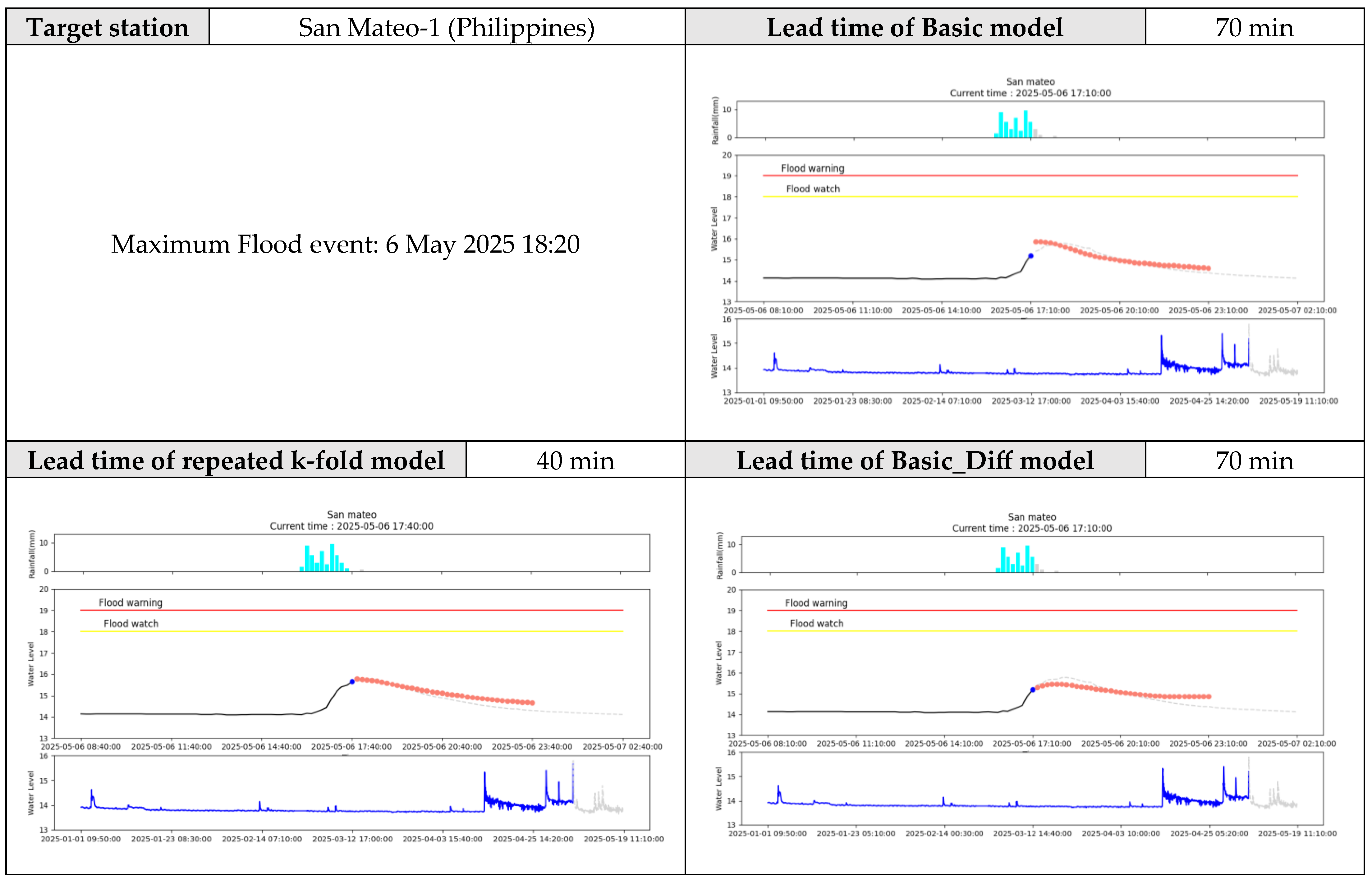
For the San Mateo-1 target station in the Philippines, the basic model predicted a maximum flood at 6 May 2025 17:10, 70 min before the maximum event occurrence time of 6 May 2025 18:20. The repeated k-fold model predicted the flood 40 min earlier, and the Basic_diff model predicted the flood 70 min earlier (Figure 13).

Figure 13. Results of water-level prediction for San Mateo-1 (Philippines) (: Predicted, : Observed).

For the Dayeuh Kolot target station in Indonesia, the basic model failed to predict floods before the maximum event time of 8 March 2025 22:50. The repeated k-fold model predicted flooding 130 min earlier, and the Basic_diff model predicted flooding 330 min earlier (Figure 14). The overall suitability was the highest for the repeater k-fold model, whereas the predicted lead time for the maximum flood event was the highest for the Basic_diff model.

Figure 14. Results of water-level prediction for Dayeuh Kolot (Indonesia) (: Predicted, : Observed).

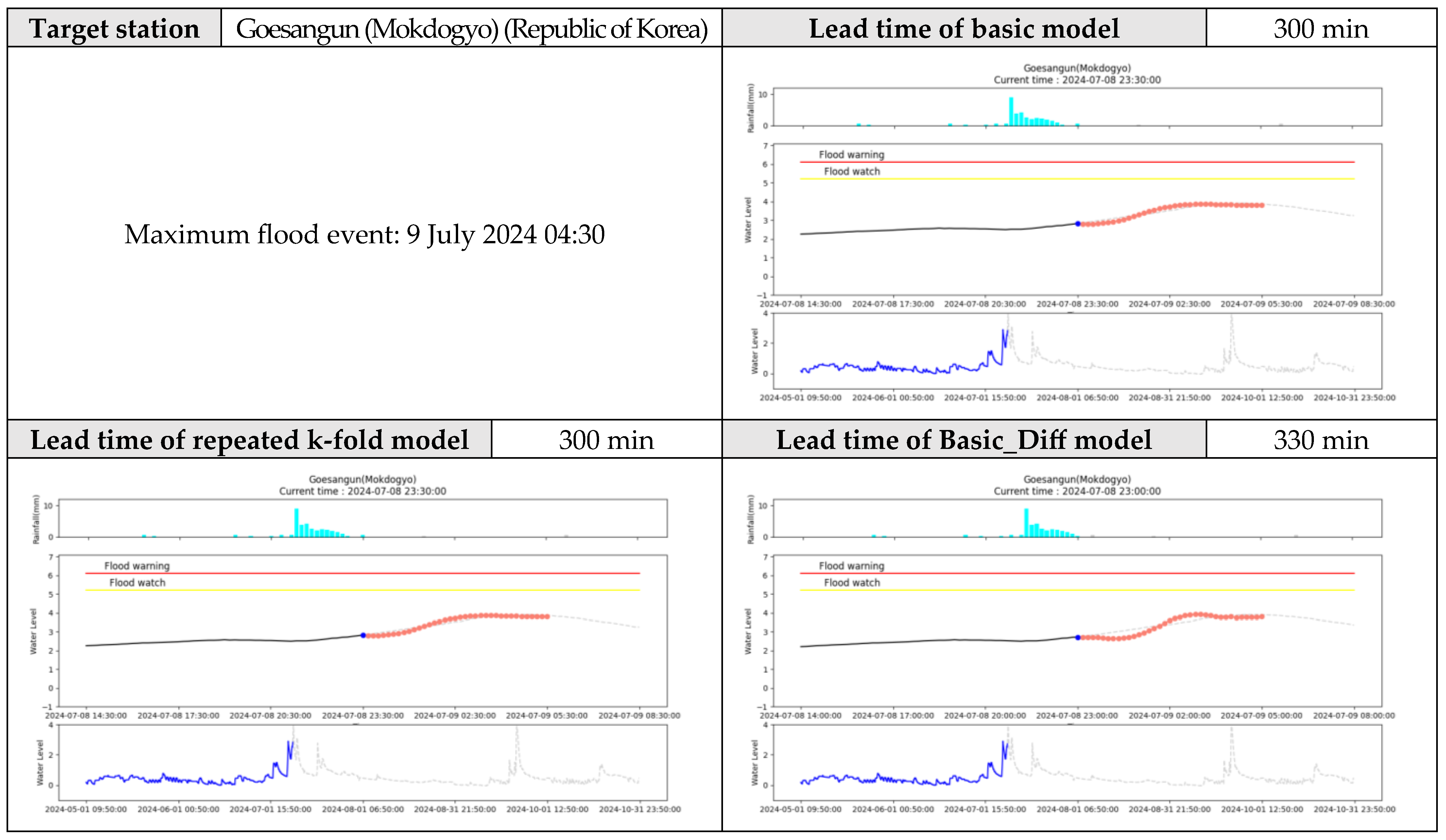
For the Goesangun (Mokdogyo) target station in the Republic of Korea, the basic model predicted the maximum flood at 8 July 2024 23:30, which is 300 min before the maximum event occurrence time of 9 July 2024 04:30. The repeated k-fold model predicted flooding 300 min earlier, and the Basic_diff model predicted flooding 330 min earlier (Figure 15). Similar to the analysis of the NSE values, repeated k-fold cross–validation exerted a minimal effect, and converting the stationary time series improved the flood prediction lead time.

Figure 15. Results of water-level prediction for Goesangun (Mokdogyo) (Republic of Korea) (: Predicted, : Observed).

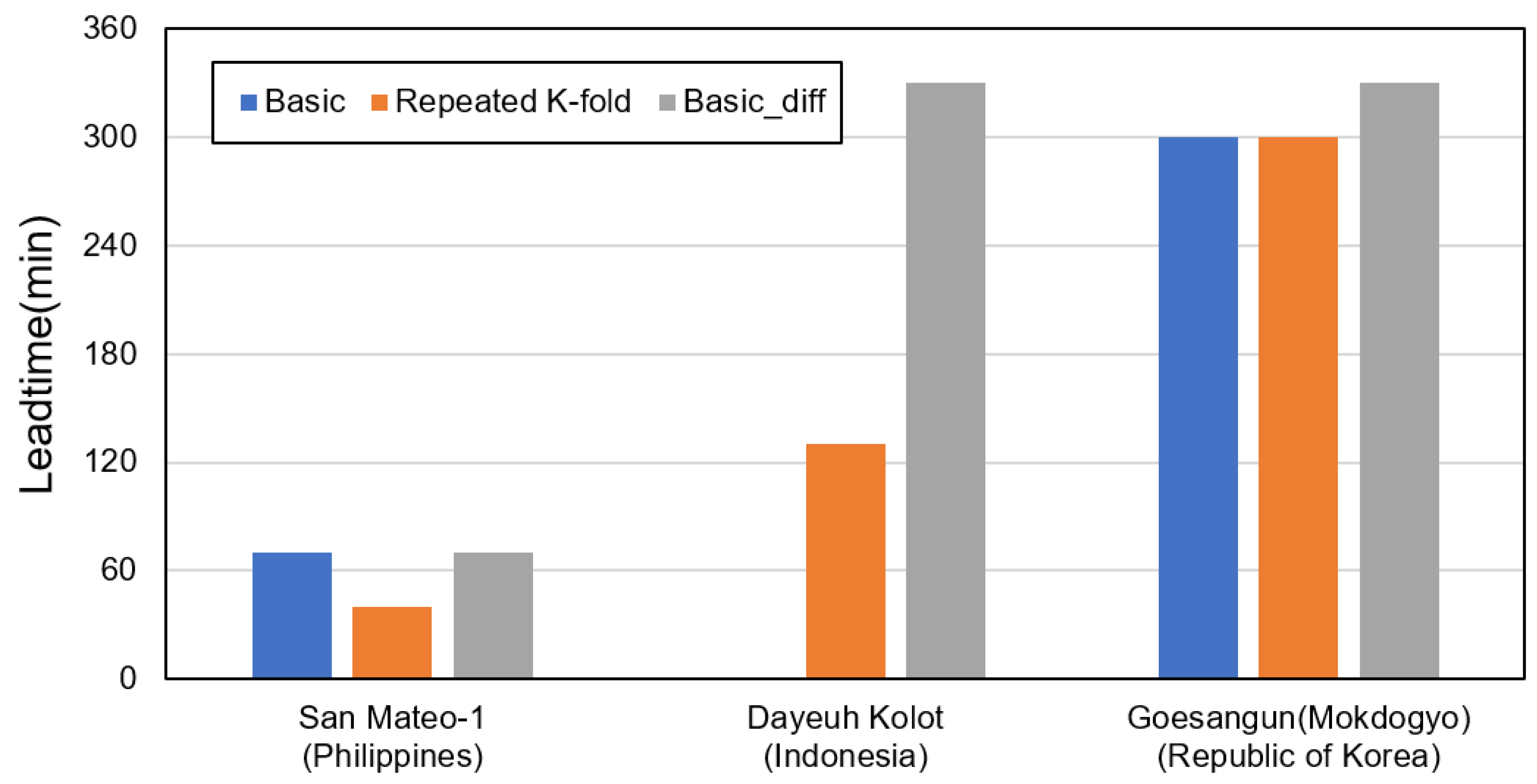
The flood prediction lead-time by model type for each target station is shown in Figure 16. The San Mateo-1 target station exhibited a predicted lead time of approximately 1 h. The lead time increased to 330 min when the data were converted into a stationary time series for the Dayeuh Kolot target station. The overall prediction accuracy was high for the Goesangun (Mokdogyo) target station. When converted to a stationary time series, both the NSE value and flood prediction lead-time exhibited maximum performance. If the observation data period is sufficiently secured and numerous reference stations can be utilized, the accuracy of river water-level predictions can be improved. The findings confirmed that more stable and accurate results can be derived through conversion to a stationary time series. Water-level differencing enhances stationarity, enabling stable training, even when hydrological inputs are highly nonlinear or seasonal.

Figure 16. Comparison of flood-prediction lead time by model type at each target station.

In addition, if the observation data period is not sufficiently secured, the accuracy can be improved using an appropriate cross-validation method. Although simple single-fold training can result in a biased performance in data-poor regions, the repeated k-fold structure enables balanced training across the folds.

6. Conclusions

In this study, various reviews were performed to construct an AI-based river water-level prediction model. First, pilot subjects were selected based on various conditions in the three countries. The proposed LSTM-based models were applied to predict the river water levels at observation stations in Korea, Indonesia, and the Philippines. Three model configurations were compared: the basic, repeated k-fold, and differenced (Basic_diff).

The effects of cross-validation and conversion of the stationary time series of the prediction data on the prediction accuracy were examined for target stations with different characteristics. The results obtained were as follows: in the case of the San Mateo-1 target station in the Philippines, which featured a few reference stations and a short observation period, the NSE value increased slightly when repeated k-fold cross-validation was performed and prediction data were converted into stationary time series; however, the flood prediction lead time for the maximum flood event improved significantly. In the case of the Dayeuh Kolot target station in Indonesia, the observation period was the shortest among the three target stations; however, numerous water-level stations and rainfall stations could be referenced upstream. Nonetheless, flood prediction was impossible using basic models. Meanwhile, repeated k-fold cross-validation and conversion of the stationary time series of the prediction data significantly improved the flood prediction lead time. In the case of Goesangun (Mokdogyo) in the Republic of Korea, an accurate prediction model was created owing to the numerous reference stations and long observation periods. The effect of repeated k-fold cross-validation was minimal, and the accuracy of flood prediction could be improved by converting the stationary time series of the prediction data.

The differenced LSTM model achieved an RMSE of 0.13 m, coefficient of determination (R²) of 0.866, NSE of 0.844, and a KGE of 0.893, outperforming the non-differenced baseline by approximately 17%. The repeated k-fold validation approach was particularly effective when the training data period was short or the number of input variables was limited. These results confirm that ensuring temporal stationarity and applying repeated cross-validation can significantly enhance the predictive accuracy of real-time flood forecasting.

Sufficient observation periods and reference stations were secured for all the AI-based models. In addition, the quality of the observed data significantly affected the accuracy of the flood prediction model. Therefore, high-quality observational data must first be obtained. Flood prediction accuracy can be improved through appropriate prediction algorithms, cross-validation, and data-type conversion. As confirmed in this study, cross-validation can improve the prediction accuracy when the observation data period is short. This is similar to the results obtained by Yaseen et al. [26], who improved the prediction accuracy through cross-validation in a short-term observational data environment. In all cases, converting the stationary time series of the predicted data yielded significant improvements in the accuracy. This analysis is consistent with that of Mosavi et al., who analyzed previous studies and found that data normalization and time series normalization contributed to an improved AI model performance [7].

AI-based river water-level prediction models can rapidly predict water levels in real time. However, prediction accuracy may decrease significantly when the observed data are affected by human actions. Therefore, when determining whether the application of an AI flood prediction model is possible and appropriate, the stability of securing observational data and data quality must be comprehensively assessed. As shown by the results of this study, region-specific model training further confirmed that the proposed framework can maintain predictive reliability across varying data lengths and hydrological conditions in the Philippines, Indonesia, and Republic of Korea. These findings validate the adaptability of the flood prediction model using AI to diverse climatic and geographical conditions. If various prediction techniques are applied to improve the accuracy of AI flood prediction models, and the optimal application conditions for each location are reviewed, more stable and accurate AI flood prediction models can be established.

References

- Kuzma, S.; Luo, T. The Number of People Affected by Floods Will Double Between 2010 and 2030; World Resources Institute: Washington, DC, USA, 2020. [Google Scholar]
- Beven, K.J. Rainfall-Runoff Modelling: The Primer; John Wiley & Sons: Hoboken, NJ, USA, 2012. [Google Scholar]
- Singh, V.P. Computer Models of Watershed Hydrology; Water Resources Publications: Littleton, CO, USA, 1995. [Google Scholar]
- Krzysztofowicz, R. Bayesian theory of probabilistic forecasting via deterministic hydrologic model. Water Resour. Res. 1999, 35, 2739–2750. [Google Scholar] [CrossRef]
- Shrestha, D.L.; Solomatine, D.P. Machine learning approaches for estimation of prediction interval for the model output. Neural Netw. 2006, 19, 225–235. [Google Scholar] [CrossRef] [PubMed]
- Abrahart, R.J.; See, L.M.; Solomatine, D.P. Practical Hydroinformatics: Computational Intelligence and Technological Developments in Water Applications; Springer Science & Business Media: Berlin, Germany, 2008; Volume 68. [Google Scholar]
- Mosavi, A.; Ozturk, P.; Chau, K.W. Flood prediction using machine learning models: Literature review. Water 2018, 10, 1536. [Google Scholar] [CrossRef]
- Kratzert, F.; Klotz, D.; Brenner, C.; Schulz, K.; Herrnegger, M. Rainfall-runoff modelling using long short-term memory (LSTM) networks. Hydrol. Earth Syst. Sci. 2018, 22, 6005–6022. [Google Scholar] [CrossRef]
- Xiang, Z.; Yan, J.; Demir, I. A rainfall-runoff model with LSTM-based sequence-to-sequence learning. Water Resour. Res. 2020, 56, e2019WR025326. [Google Scholar] [CrossRef]
- Hu, C.; Wu, Q.; Li, H.; Jian, S.; Li, N.; Lou, Z. Deep learning with a long short-term memory networks approach for rainfall-runoff simulation. Water 2018, 10, 1543. [Google Scholar] [CrossRef]
- Le, X.H.; Ho, H.V.; Lee, G.; Jung, S. Application of long short-term memory (LSTM) neural network for flood forecasting. Water 2019, 11, 1387. [Google Scholar] [CrossRef]
- Ding, Y.; Zhu, Y.; Feng, J.; Zhang, P.; Cheng, Z. Interpretable spatio-temporal attention LSTM model for flood forecasting. Neurocomputing 2020, 403, 348–359. [Google Scholar] [CrossRef]
- Fang, Z.; Wang, Y.; Peng, L.; Hong, H. Predicting flood susceptibility using LSTM neural networks. J. Hydrol. 2021, 594, 125734. [Google Scholar] [CrossRef]
- Kim, S.; Kim, H.J.; Yoon, K.S. Development of artificial intelligence-based river flood level prediction model capable of independent self-warning. J. Korea Water Resour. Assoc. 2021, 54, 1285–1294. [Google Scholar]
- Zhang, Y.; Zhou, Z.; Van Griensven Thé, J.; Yang, S.X.; Gharabaghi, B. Flood forecasting using hybrid LSTM and GRU models with lag time preprocessing. Water 2023, 15, 3982. [Google Scholar] [CrossRef]
- Oddo, P.C.; Bolten, J.D.; Kumar, S.V.; Cleary, B. Deep Convolutional LSTM for improved flash flood prediction. Front. Water 2024, 6, 1346104. [Google Scholar] [CrossRef]
- De la Fuente, L.A.; Ehsani, M.R.; Gupta, H.V.; Condon, L.E. Towards interpretable LSTM-based modelling of hydrological systems. Hydrol. Earth Syst. Sci. 2024, 28, 945–971. [Google Scholar] [CrossRef]
- Malik, H.; Feng, J.; Shao, P.; Abduljabbar, Z.A. Improving flood forecasting using time-distributed CNN-LSTM model: A time-distributed spatiotemporal method. Earth Sci. Inform. 2024, 17, 3455–3474. [Google Scholar] [CrossRef]
- Graves, A. Long short-term memory. In Supervised Sequence Labelling with Recurrent Neural Networks; Springer: Berlin/Heidelberg, Germany, 2012; Volume 385, pp. 37–45. [Google Scholar]
- Olah, C. Understanding Lstm Networks. Available online: https://colah.github.io/posts/2015-08-Understanding-LSTMs/ (accessed on 23 November 2021).
- Wong, T.T.; Yeh, P.Y. Reliable accuracy estimates from k-fold cross validation. IEEE Trans. Knowl. Data Eng. 2019, 32, 1586–1594. [Google Scholar] [CrossRef]
- Marcot, B.G.; Hanea, A.M. What is an optimal value of k in k-fold cross-validation in discrete Bayesian network analysis? Comput. Stat. 2021, 36, 2009–2031. [Google Scholar] [CrossRef]
- Liu, Y.; Wu, H.; Wang, J.; Long, M. Non-stationary transformers: Exploring the stationarity in time series forecasting. Adv. Neural Inf. Process. Syst. 2022, 35, 9881–9893. [Google Scholar]
- Krause, P.; Boyle, D.P.; Bäse, F. Comparison of different efficiency criteria for hydrological model assessment. Adv. Geosci. 2005, 5, 89–97. [Google Scholar] [CrossRef]
- Moriasi, D.N.; Gitau, M.W.; Pai, N.; Daggupati, P. Hydrologic and water quality models: Performance measures and evaluation criteria. Trans. ASABE 2015, 58, 1763–1785. [Google Scholar] [CrossRef]
- Yaseen, Z.M.; El-Shafie, A.; Jaafar, O.; Afan, H.A.; Sayl, K.N. Artificial intelligence based models for stream-flow forecasting: 2000–2015. J. Hydrol. 2015, 530, 829–844. [Google Scholar] [CrossRef]
Figure 1.
Schematics of RNN and LSTM [
20].
Figure 2.
Diagram showing procedure for calculating repeated k-folds (■: Training data, ■: Test data).
Figure 3.
Stationary evaluation of water-level differencing convert.
Figure 4.
Calculation of difference between predicted water levels by lead time.
Figure 5.
Location map of San Mateo-1 and reference stations in the Philippines.
Figure 6.
Location map of Dayeuh Kolot and reference stations in Indonesia.
Figure 7.
Location map of Goesangun (Mokdogyo) and reference stations in Republic of Korea.
Figure 8.
Preprocessing of water-level data in San Mateo-1 (Philippines) (example).
Figure 9.
Dataset composition for AI-prediction model learning) (––: water-level, ––: rainfall).
Figure 10.
Calculation procedure for AI prediction model.
Figure 11.
Results of test process for trained model.
Figure 12.
Comparison of model performance.
Figure 13.
Results of water-level prediction for San Mateo-1 (Philippines) (
![Earth 06 00146 i007 Earth 06 00146 i007]()
: Predicted,
![Earth 06 00146 i008 Earth 06 00146 i008]()
: Observed).
Figure 14.
Results of water-level prediction for Dayeuh Kolot (Indonesia) (
![Earth 06 00146 i009 Earth 06 00146 i009]()
![Earth 06 00146 i010 Earth 06 00146 i010]()
Figure 15.
Results of water-level prediction for Goesangun (Mokdogyo) (Republic of Korea) (
![Earth 06 00146 i011 Earth 06 00146 i011]()
![Earth 06 00146 i012 Earth 06 00146 i012]()
Figure 16.
Comparison of flood-prediction lead time by model type at each target station.