Machine Learning for Predicting Coliform Concentrations at Montevideo Beaches: Identifying Key Environmental Drivers for Coastal Water Quality Management

Abstract

Monitoring microbial water quality at recreational beaches is essential to safeguard public health, with fecal coliforms serving as key indicators of contamination. This study applies machine learning (ML) techniques to predict fecal coliform concentrations at Montevideo’s urban beaches, aiming to support proactive and data-driven coastal water quality management. Using an extensive monitoring dataset, we developed and calibrated five ML models to predict continuous fecal coliform levels, improving upon traditional threshold-based methods. Among these, Random Forest (RF) and Histogram-based Gradient Boosting (HGB) models showed very good predictive performance, with RF yielding the most consistent estimates of microbial contamination and HGB showing comparable accuracy but higher predictive uncertainty. The models were optimized using cross-validation and Optuna, with mean squared error as the loss function. Feature importance analysis using SHAP values revealed that Enterococcus concentrations were the most influential predictor, followed by water temperature and salinity. Seasonal patterns in coliform levels were also identified, likely linked to fluctuations in water temperature. These findings provide actionable insights into the dynamics of microbial contamination and highlight the potential of ML models for early warning systems, adaptive monitoring, and improved risk communication. This integrative approach not only enhances predictive performance but also advances our understanding of the environmental processes influencing water quality in urban coastal systems.

1. Introduction

Monitoring microbial water quality at recreational beaches is essential to safeguard public health [1]. Among microbial indicators, coliform bacteria, particularly Escherichia coli and fecal coliforms, are widely used to assess fecal contamination and the potential presence of pathogenic microorganisms in surface waters [2]. These indicators are especially relevant in coastal urban areas, where pollution from stormwater runoff, combined sewer overflows, and diffuse sources may lead to fluctuating levels of contamination [3].

Exposure to elevated coliform concentrations during recreational activities has been associated with an increased risk of gastrointestinal, respiratory, and dermatological illnesses [4]. Vulnerable populations, such as children, the elderly, and immunocompromised individuals, are particularly at risk. In response, international guidelines, including those from the World Health Organization [5] and regional frameworks such as MERCOSUR [6], have established thresholds for acceptable microbial contamination levels. In Uruguay, these thresholds are enforced through routine monitoring along the country’s most frequented recreational beaches [7].

Montevideo’s urban coastline, which stretches over 20 km along the Río de la Plata estuary, is home to several popular beaches that are intensively used, especially during the summer months. However, these beaches are subject to multiple contamination pressures, including urban runoff, sewer overflows, and drainage discharges, particularly during and after rainfall events. As a result, microbial contamination can vary significantly in space and time, posing challenges to public health authorities responsible for water quality monitoring and risk communication [8].

Traditional monitoring methods rely on manual sampling and laboratory-based analyses, which, although accurate, often involve significant time lags and limited spatial coverage. These constraints can delay public health advisories and hinder effective, real-time management of beaches. To overcome these limitations, recent research has begun to explore data-driven approaches that leverage environmental, meteorological, and hydrological information to anticipate contamination events [9,10,11,12]. In this context, machine learning (ML) techniques have emerged as powerful tools for predicting microbial water quality, offering the potential for faster, more adaptive, and spatially comprehensive assessments [13,14,15].

Several studies have focused on developing predictive models to support water quality management in Montevideo’s coastal areas, particularly its recreational beaches [16,17,18,19]. Segura et al. [16] applied ML techniques to predict exceedances of fecal coliform concentrations (i.e., FC > 2000) using a decade of high-quality monitoring data. By incorporating in situ, meteorological, and oceanographic variables, they trained various ML models and found that stratified Random Forest outperformed other algorithms, achieving 86% overall accuracy and a 60% improvement in true positive rates compared to a baseline model. Bourel et al. [19] addressed the specific challenge of predicting rare contamination events from highly imbalanced datasets, which are common in recreational water quality data. Their study introduced and evaluated several ML approaches, including Synthetic Minority Oversampling Technique (SMOTE) and stratified Random Forest, showing that data pre-treatment is essential to improve model sensitivity. Their findings highlighted the limitations of traditional accuracy metrics for imbalanced problems and suggested alternative evaluation metrics, such as true positive and false positive rates. Among 52 tested algorithms, Random Forest and SVMs with appropriate resampling techniques yielded the best results. In a broader ecological modeling context, Bourel et al. [17] explored the use of consensus methods that combine multiple binary classifiers (e.g., GLM, RF, SVM, Boosting) to predict the presence or absence of marine phytoplankton species. Some of these species have implications for coastal water quality and public perception due to toxicity or discoloration. Their weighted average consensus model consistently achieved the lowest classification errors across diverse datasets, including marine phytoplankton and benchmark open-access datasets. Bourel and Segura [18] extended the application of ML to multiclass ecological classification problems, introducing seven multiclass classification algorithms and assessing their performance using both simulated and real phytoplankton data. Their results highlighted how the structure of the data influences algorithm selection and predictive performance. Notably, Random Forest, SAMME boosting, and consensus logistic regression models showed high accuracy, while interpretability and generalization error were emphasized as key criteria for model selection in ecological applications.

While the aforementioned studies have demonstrated the potential of ML models for classification tasks, particularly in identifying exceedance events of fecal coliform thresholds, the predictive modeling of actual concentration values remains less explored. While previous studies in Montevideo [16,18] have primarily focused on threshold-based classifications to assess bathing water quality, the present work advances this line of research by modeling continuous fecal coliform concentrations, enabling a more nuanced representation of contamination variability across space and time.

Furthermore, most existing studies prioritize model performance metrics without thoroughly examining the interpretability or explanatory power of the [20]. In particular, the identification and ranking of the most influential predictor variables in determining coliform levels is an underdeveloped area of research. Understanding which environmental, meteorological, or oceanographic variables most strongly drive contamination dynamics can inform targeted monitoring efforts and resource allocation and support the development of mechanistic hypotheses regarding pollution sources and transport pathways.

Our study aims to address these gaps by (i) developing ML models to predict fecal coliform concentrations as continuous variables across selected Montevideo beaches, (ii) evaluating the predictive utility of these models for practical water quality management, and (iii) analyzing the relative importance of input features to uncover key drivers of microbial contamination. This integrated approach aims to enhance predictive performance and generate actionable insights into the environmental processes that underlie water quality variability in urban coastal systems.

Beyond the application of machine learning to Montevideo data, this work constitutes the first continuous (non-threshold) prediction of coliform levels for Uruguayan beaches, advancing the use of explainable machine learning for microbial risk management and offering a transferable framework for other coastal systems.

2. Material and Methods

2.1. Water Quality and Meteorological Data

2.1.1. Water Quality Information

For this study, we utilized water quality data from the Intendencia de Montevideo (IM) monitoring program, which regularly assesses the water quality at the city’s beaches to ensure public health and support effective beach management. The IM’s Servicio de Evaluación de la Calidad y Control Ambiental (SECCA) conducts year-round water quality monitoring along the urban coastline of Montevideo, which spans 530 km², 40% of which is urbanized. The city’s coastline stretches across the Río de la Plata and includes approximately 15 of the 70 km of beach arcs within the department [21].

During the summer, the IM performs regular water quality sampling four times a week, with one sample being randomly selected as mandatory, ensuring data collection regardless of weather conditions, including rainfall. Additionally, water samples are collected from coastal discharges, including stormwater outlets, streams, and creeks that flow into each beach. Other samples are taken only when no discharges have occurred in the previous 24 h [21].

For the purpose of our study, we focused on beaches with more than 900 data points, ensuring sufficient temporal coverage and representation of variability for robust model development (

Table 1. Number of samples collected at each beach monitored by IM.

Beach	Number of Samples
Pocitos	1408
Malvín	1407
Cerro	1401
Ramírez	1399
Pajas Blancas	1010
Carrasco	996
Ingleses	5
Santa Catalina	2
Punta Espinillo	2
Buceo	2

). This threshold was chosen to balance the need for a consistent and sizable dataset while retaining a representative subset of the monitored beaches. Previous studies have shown that machine learning models for environmental prediction typically require several hundred observations to capture seasonal patterns, detect rare events, and ensure generalizability [22,23]. The selected beaches were Pocitos (1408 data points), Malvín (1407 data points), Del Cerro (1401 data points), Ramírez (1399 data points), Pajas Blancas (1010 data points), and Carrasco (996 data points) (Figure 1).

These beaches were selected for their extensive datasets, which enable a more robust statistical analysis of microbial contamination patterns over time. Data include coliform concentrations (CFU/100 mL), salinity (PSU), water temperature (°C), and enterococcus (CFU/100 mL). Additionally, each water quality data point is classified as either Representative or Non-Representative. Samples are labeled Representative when no rainfall-induced discharges occurred in the 24 h preceding sampling. In contrast, they are marked as Non-Representative when precipitation events result in discharges, rendering the samples unrepresentative of normal conditions. Figure 1 shows the locations of the beaches selected for this study along the Montevideo coastline.

2.1.2. Meteorological Information

Meteorological data used in this study were obtained from the Agroclimatic Database of the National Institute of Agricultural Research (INIA) [24]. The data were collected at the INIA Las Brujas meteorological station, located approximately 35 km northwest of Montevideo (Figure 1). This station provides high-quality, daily monitored weather information representative of the study area.

The variables considered for model development included accumulated daily precipitation (mm), mean air temperature (°C), relative humidity (%), solar radiation (cal/cm²), and wind speed (km/day).

2.2. Data Analysis

Before implementing the machine learning models, we performed an Exploratory Data Analysis (EDA). This step was essential for gaining a better understanding of the distribution and behavior of fecal coliform concentrations across the selected beaches, identifying any potential outliers, and supporting the selection of relevant predictor variables for model development. The goal was to ensure that redundant or highly correlated features did not mask key relationships between environmental variables and coliform levels.

EDA was conducted using Python (version 3.10) tools, including the pandas-profiling (version 3.6.6) package, which provided an automated overview of the dataset. Given the non-linear nature of the environmental processes involved, we relied primarily on Spearman’s rank correlation to assess monotonic relationships between variables. To complement this, we also computed the Kendall correlation coefficient, which provided additional insights, particularly in cases where relationships were either non-linear or involved categorical data.

Correlation matrices were visualized through heatmaps, where darker shades indicated stronger associations, whether positive or negative. These visual tools helped screen for multicollinearity among input features, enabling a more informed selection of the final set of predictors to be used in model training.

In addition, to harmonize the scales of the input variables, since they differed in units and magnitude, we applied a min-max normalization, transforming all variables into a common range of [0, 1]. This step was necessary to ensure that no single variable dominated the learning process due to its scale. The normalization was performed using the MinMaxScaler from the sklearn.preprocessing module, as all input features were strictly positive and no significant outliers were detected.

2.3. Machine Learning Models

We evaluated five regression models of varying complexity to predict fecal coliform concentrations, using Linear Regression as the baseline. Linear Regression (LR) is a simple, interpretable model that assumes a linear relationship between input features and the target variable. It serves as a benchmark to assess the relative performance improvements offered by more complex models.

Support Vector Regressor (SVR) maps the input data into a high-dimensional space using kernel functions. It seeks to find a function that approximates the data within a specified error margin. SVR is known for its robustness to outliers and flexibility in capturing non-linear relationships.

The Decision Tree Regressor (DTR) is a non-parametric model that recursively splits the input space into regions based on feature values, resulting in a tree structure. It can capture non-linear patterns and interactions, but is prone to overfitting if not properly constrained.

Random Forest Regressor (RFR) is an ensemble method that constructs multiple decision trees and outputs the average prediction, reducing overfitting and improving generalization. It enhances the stability and accuracy of decision trees by introducing randomness in both feature selection and the selection of sample subsets.

Histogram-Based Gradient Boosting Regressor (HGBR) is a highly efficient and scalable implementation of gradient boosting that bins continuous features into histograms for faster training. It builds additive models in a forward stage-wise fashion, optimizing a loss function through gradient descent, and is particularly suited for large datasets and complex non-linear relationships.

2.4. Model Optimization and Performance Evaluation

To ensure robust model performance and prevent overfitting, we implemented a structured model optimization workflow [25]. The dataset was randomly divided into 80% for training and 20% for testing. This split ensured that the models were trained on a representative subset of the data while retaining an independent portion for unbiased evaluation. Model calibration was conducted using 5-fold cross-validation within the training set, which provided a reliable estimate of generalization performance and helped tune hyperparameters effectively. For this purpose, we employed Optuna [26], an efficient hyperparameter optimization framework that utilizes a Bayesian sampling strategy. The Mean Squared Error (MSE) was adopted as the loss function to guide the search for optimal model configurations.

Table 2. Hyperparameters and their respective bounds for each machine learning model. The description of the parameters can be found in Geron [27].

Model	Hyperparameter	Bounds
SVR	C	$[1\times {10}^{-3},1\times {10}^3]$
	gamma	{scale, auto}
	kernel	{linear, poly, rbf, sigmoid}
	epsilon	$[0.01,0.5]$
	degree	[2, 5] (only used for ’poly’ kernel)
DTR	max_depth	$[2,30]$
	min_samples_split	[2, 20]
	min_samples_leaf	[1, 20]
	criterion	{squared_error, friedman_mse, absolute_error, poisson}
	random_state	42
RFR	n_estimators	$[50,500]$
	max_depth	$[2,30]$
	min_samples_split	[2, 20]
	min_samples_leaf	[1, 20]
	max_features	{sqrt, log2, None}
	random_state	42
HGBR	learning_rate	$[1\times {10}^{-3},0.5]$
	max_iter	$[50,1000]$
	max_leaf_nodes	[20, 100]
	max_depth	$[2,30]$
	l2_regularization	$[1\times {10}^{-10},1.0]$
	random_state	42

presents the hyperparameters used for the ML models, where each model’s hyperparameters are listed along with their corresponding bounds or possible values. The table outlines log-scale ranges for continuous parameters such as learning rates and depths, categorical options for parameters such as kernel types and criteria, and specific integer ranges for parameters such as the number of estimators and minimum sample splits.

Table 3. Performance metrics and their corresponding mathematical expressions: (1) MSE measures the average squared difference between observed ($y_i$) and predicted (${\widehat{y}}_i$) values, with lower values indicating better performance. It ranges from $[0,\infty )$. (2) NSE evaluates how well the model predictions match observed data. It ranges between $(-\infty ,1]$, with 1 being a perfect match. Values $<0$ suggest the mean of observations is a better predictor. (3) PBIAS indicates the average tendency of the predicted values to be larger or smaller than the observed ones. It ranges between $(-\infty ,\infty )$; 0 indicates a perfect model, with positive values indicating underestimation and negative values indicating overestimation.

Metric	Expression
Mean Squared Error (MSE)	${\displaystyle \mathrm{MSE}=\frac{1}{n}\sum _{i=1}^n{(y_i-{\widehat{y}}_i)}^2}$
Nash–Sutcliffe Efficiency (NSE)	${\displaystyle \mathrm{NSE}=1-\frac{{\sum }_{i=1}^n{(y_i-{\widehat{y}}_i)}^2}{{\sum }_{i=1}^n{(y_i-\overline{y})}^2}}$
Percent Bias (PBIAS)	${\displaystyle \mathrm{PBIAS}=100\times \frac{{\sum }_{i=1}^n(y_i-{\widehat{y}}_i)}{{\sum }_{i=1}^n{y}_i}}$

summarizes the mathematical expressions for each metric, providing an overview of their definitions and uses. Model performance was assessed using three standard statistical metrics: Mean Squared Error (MSE), Nash–Sutcliffe Efficiency (NSE), and Percent Bias (PBIAS). These metrics provide complementary insights into the accuracy, explanatory power, and bias of the predictions in comparison to observed values.

As a reference for interpreting the model performance metrics, we follow the guidelines proposed by Moriasi et al. [28] (

Table 4. Performance rating criteria for evaluation metrics (adapted from [22,28]).

Performance Rating	NSE	PBIAS (%)
Very Good	>0.65	<±10
Good	$0.50$–$0.65$	$\pm 10$ to $\pm 15$
Satisfactory	$0.30$–$0.50$	$\pm 15$ to $\pm 30$
Unsatisfactory	≤0.30	>±30

). Although specific guidelines for coliform concentrations are not provided, the evaluation criteria established for nutrient parameters such as phosphorus (P) or nitrogen (N) can serve as a reasonable benchmark for assessing model accuracy in this context, given their similar variability and behavior in environmental modeling applications.

To estimate model uncertainty, different strategies were applied depending on the characteristics of each machine learning model. For the RFR, epistemic uncertainty was quantified by computing the standard deviation of predictions from all individual decision trees within the ensemble. In the case of the HGBR, aleatoric uncertainty was estimated by training two additional models using quantile regression to predict the 5th and 95th percentiles, thereby deriving a 90% prediction interval. This confidence level was selected to balance coverage and interpretability, capturing most of the variability in fecal coliform predictions without being overly conservative for management applications. Since neither the DTR nor the SVR provides uncertainty estimates natively, a bootstrapping approach was employed: 100 models were trained on different resampled versions of the training data. The number of iterations was chosen as a compromise between computational efficiency and the stability of the resulting uncertainty estimates, which showed convergence beyond approximately 100 resamples. For the Linear Regression model used as a baseline, prediction intervals were computed analytically based on the standard error of the residuals under the assumption of normally distributed errors. This combination of ensemble-based, quantile-based, resampling-based, and analytical methods allowed us to consistently estimate predictive uncertainty across all models.

2.5. Feature Importance Analysis

To assess the input variables’ relative importance and enhance the model predictions’ interpretability, we carried out a feature importance analysis using SHapley Additive exPlanations (SHAP). SHAP provides a unified framework based on cooperative game theory to explain individual predictions by computing the contribution of each feature, making it applicable to a wide range of ML algorithms [29].

In this study, SHAP values were computed using the $TreeExplainer$, $KernelExplainer$, and $PermutationExplainer$ methods available in the SHAP Python package, depending on the type of model used. This allowed us to capture both linear and non-linear relationships between the predictors and the target variable, as well as to account for potential interactions among features.

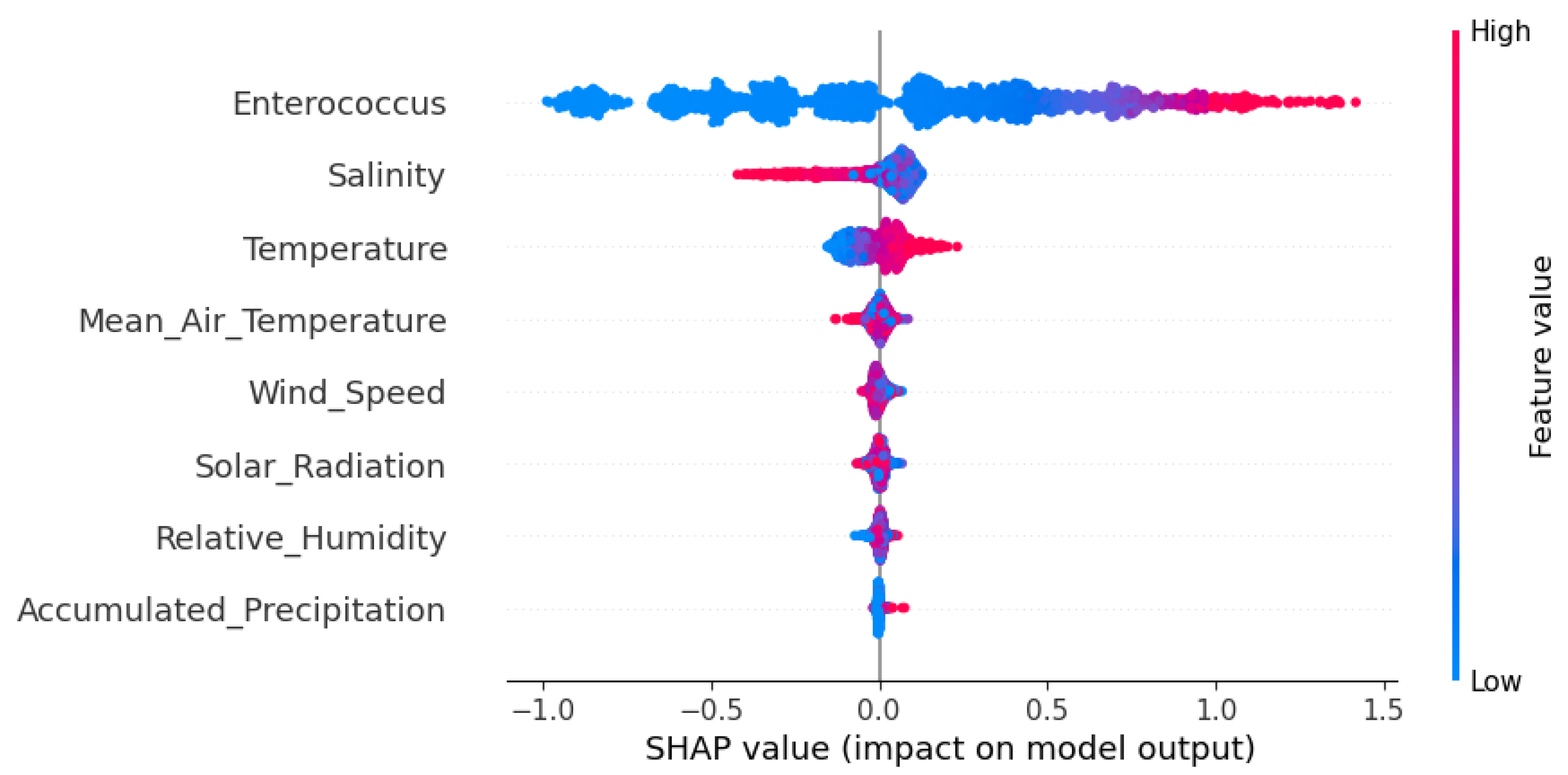
SHAP summary plots provide a compact visualization of feature importance. Each point on the plot represents a SHAP value for a given feature and a single observation. The x-axis shows the magnitude and direction of the feature’s impact on the model output (positive or negative). At the same time, the color indicates the original value of the feature (e.g., red for high values and blue for low values). Features are sorted from top to bottom by their overall importance, allowing quick identification of the most influential variables.

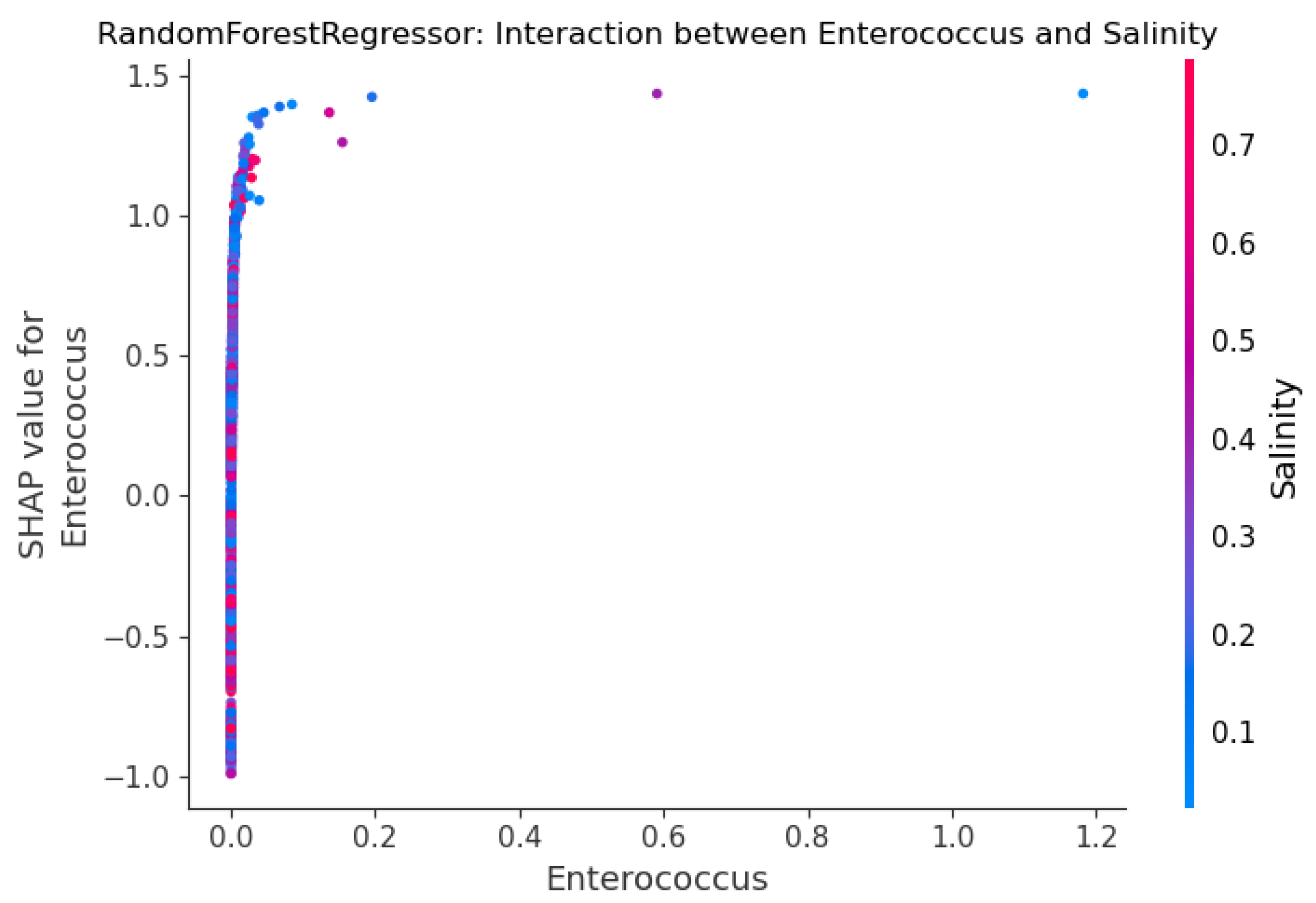
In addition, to better understand how pairs of variables jointly influence model predictions, SHAP interaction plots were generated. These plots illustrate how the SHAP value of one feature changes in response to changes in another, highlighting potential synergistic or compensatory effects between predictors. This visualization helps identify non-linear dependencies and interactions that are not easily captured by traditional importance rankings, providing deeper insight into model behavior and feature relationships.

2.6. Proposed Framework

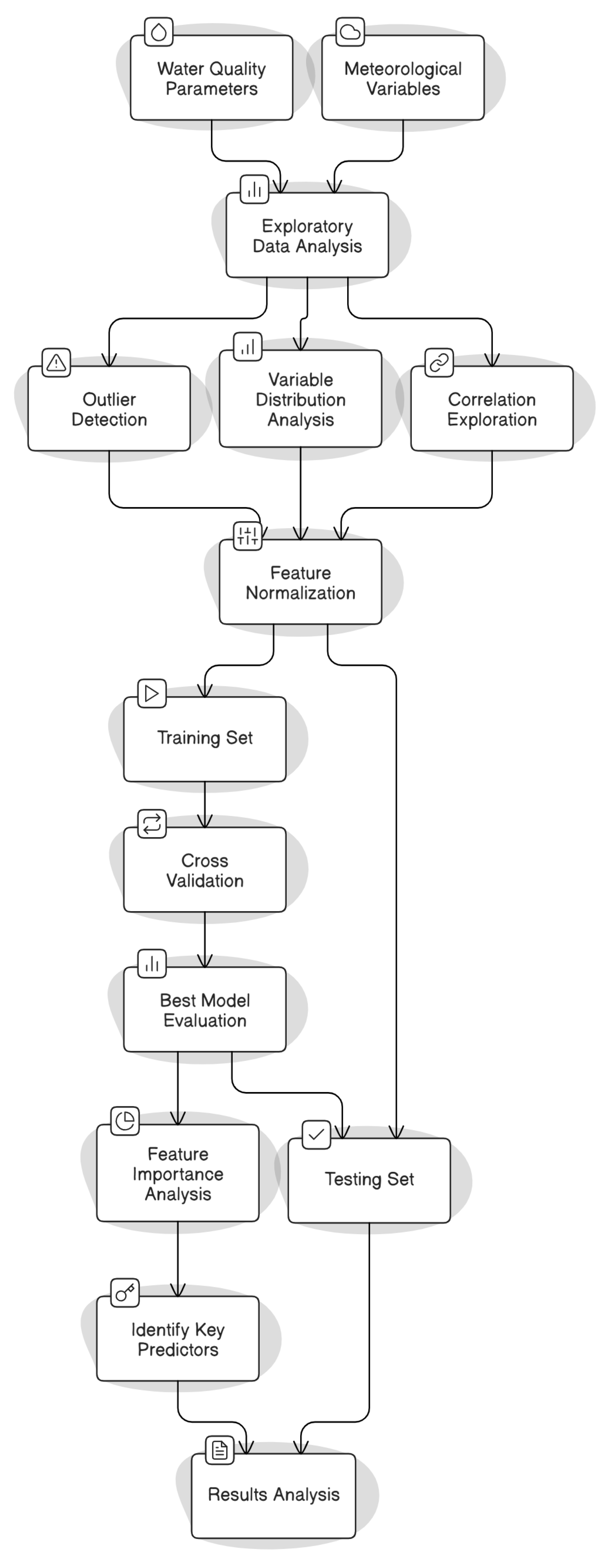
The methodological approach adopted in this study aimed to predict fecal coliform concentrations at selected recreational beaches using meteorological data and water quality indicators, with an emphasis on model interpretability, reproducibility, and practical applicability. We considered water quality parameters, including fecal coliforms, salinity, water temperature, and enterococcus, along with daily meteorological variables, including accumulated precipitation, air temperature, relative humidity, wind speed, and solar radiation. An EDA was conducted on the entire dataset to detect outliers, understand variable distributions, and explore correlations among variables. Subsequently, all features were normalized using a min-max transformation, scaling them to a standard range of [0, 1].

The normalized dataset was then used to train and test five different ML models. For all of them, the output was Log-scaled coliform concentration. To evaluate the models’ predictive performance, the dataset was randomly split into 80% for training and 20% for testing. The training process included hyperparameter tuning using 5-fold cross-validation, which allowed for model optimization and reduced the risk of overfitting. Once the best parameters were identified, the final models were retrained on the whole training set and evaluated on the test set using performance metrics such as the NSE, RMSE, and MAE. These metrics provided a comprehensive understanding of each model’s ability to generalize to new, unseen data.

To assess the influence of each input variable on model predictions, we conducted a feature importance analysis using SHAP, which enabled the interpretation of individual model outputs and the identification of the most relevant predictors.

All steps were designed with reproducibility in mind: code and data workflows were managed via a GitHub repository, ensuring transparency and replicability. Finally, the results were analyzed in the context of water safety and public health, with the aim of deriving policy-relevant insights to support beach management and water quality advisories.

The workflow of the methodology conceptualization adopted in this study is reported in Figure 2.

3. Results

3.1. Exploratory Data Analysis

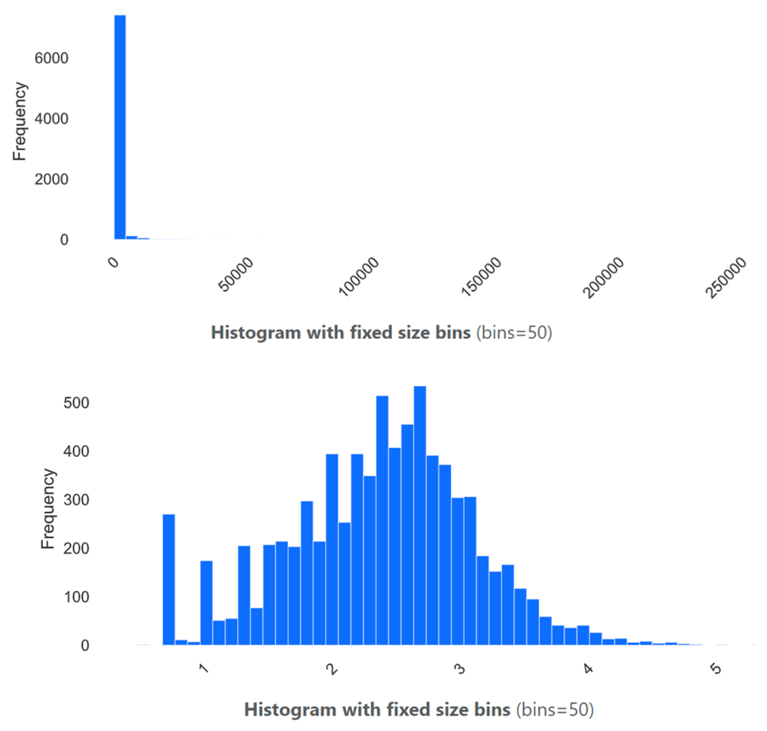
The distribution of fecal coliform concentrations reveals a non-stationary, highly skewed, and seasonal behavior (Figure 3). To address the pronounced skewness and heteroscedasticity observed in the raw fecal coliform concentrations, a base 10-logarithmic transformation was applied (Log). The resulting distribution (Figure 3) exhibits a notable improvement in symmetry and spread, facilitating more straightforward interpretation and more robust statistical modeling. After transformation, the mean and median values are 2.37 and 2.43 (in Log CFU/100 mL), respectively, indicating a much lower skewness (−0.18), in contrast to the original skewness of 31.74. The kurtosis also dropped substantially from 1609.83 to 0.06, indicating the absence of heavy tails and a distribution closer to normality.

The coefficient of variation decreased from 4.45 to 0.31, and the standard deviation dropped from 4092.22 to 0.73, reflecting a significant reduction in variability relative to the mean. Additionally, extreme values no longer dominate the distribution: the interquartile range (IQR) shrinks from 610 to 0.94, and the range reduces from 239,997 to 4.90. These changes suggest that the log-transformed data is not only easier to visualize but also more appropriate for statistical analysis and modeling, especially under assumptions of normality or homoscedasticity.

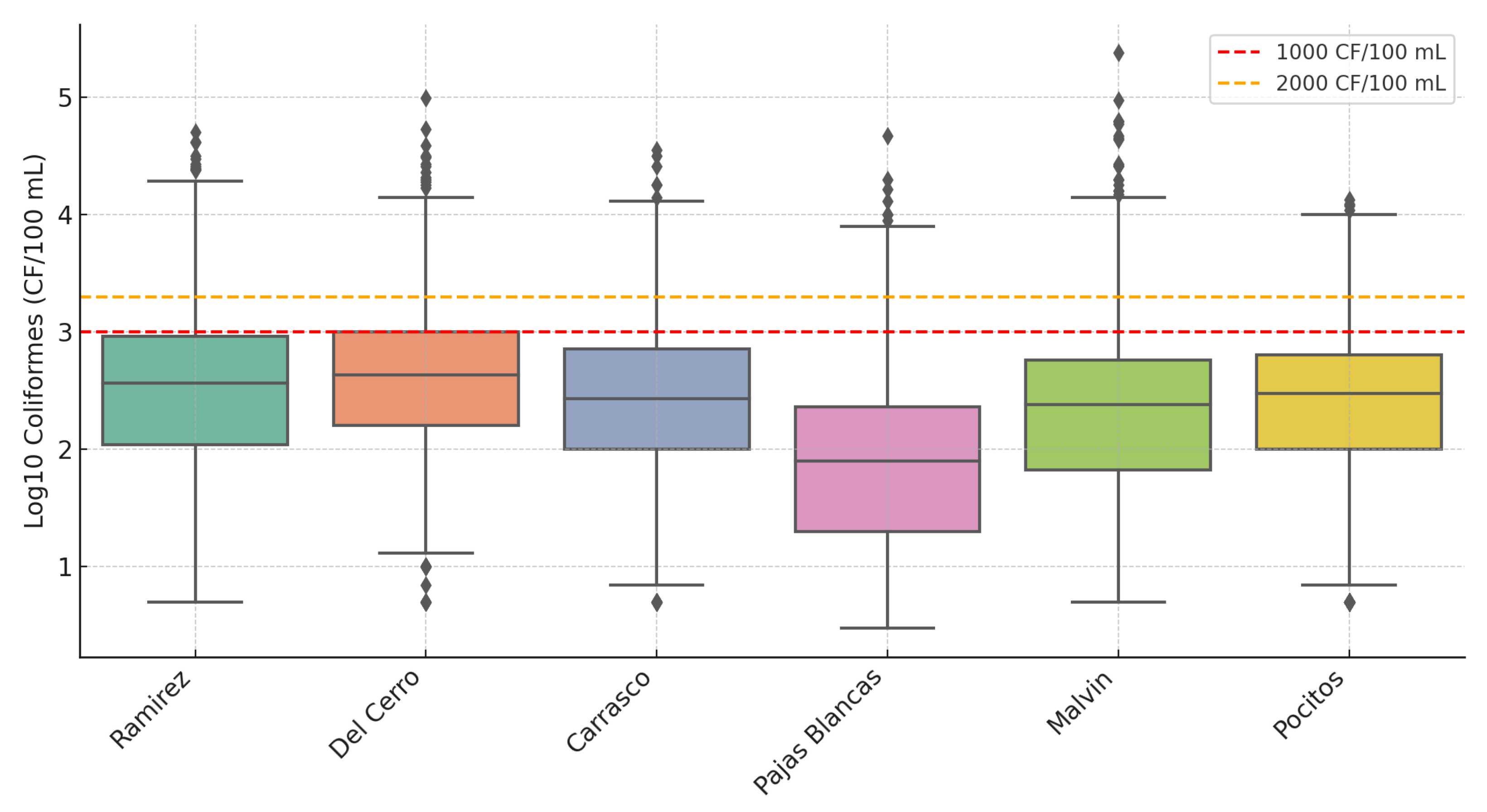
In Log scale, differences in lower and moderate concentrations become visible, making trends easier to detect and interpret. This transformation helps mitigate the impact of extreme values, allowing both central tendencies and variability to be evaluated more accurately. In Figure 4, the boxplot of Log-transformed thermotolerant coliform concentrations is presented for each selected beach. To contextualize these results, we compare the observed values with Uruguay’s bathing water quality standards established by the Ministry of Environment. According to national regulations (Decree No. 253/79 and its amendments, RM s/n of 25 February 2005, and the Gesta Agua proposal) [30], waters classified as Class 3 must meet two key microbiological criteria: (i) individual samples should not exceed 2000 CFU/100 mL, and (ii) the geometric mean of at least five samples must remain below 1000 CFU/100 mL. In Figure 4, these thresholds are indicated by horizontal dashed lines, allowing a visual assessment of compliance. The distribution of Log-coliform levels varies markedly among beaches, highlighting spatial disparities in water quality and potential health risks.

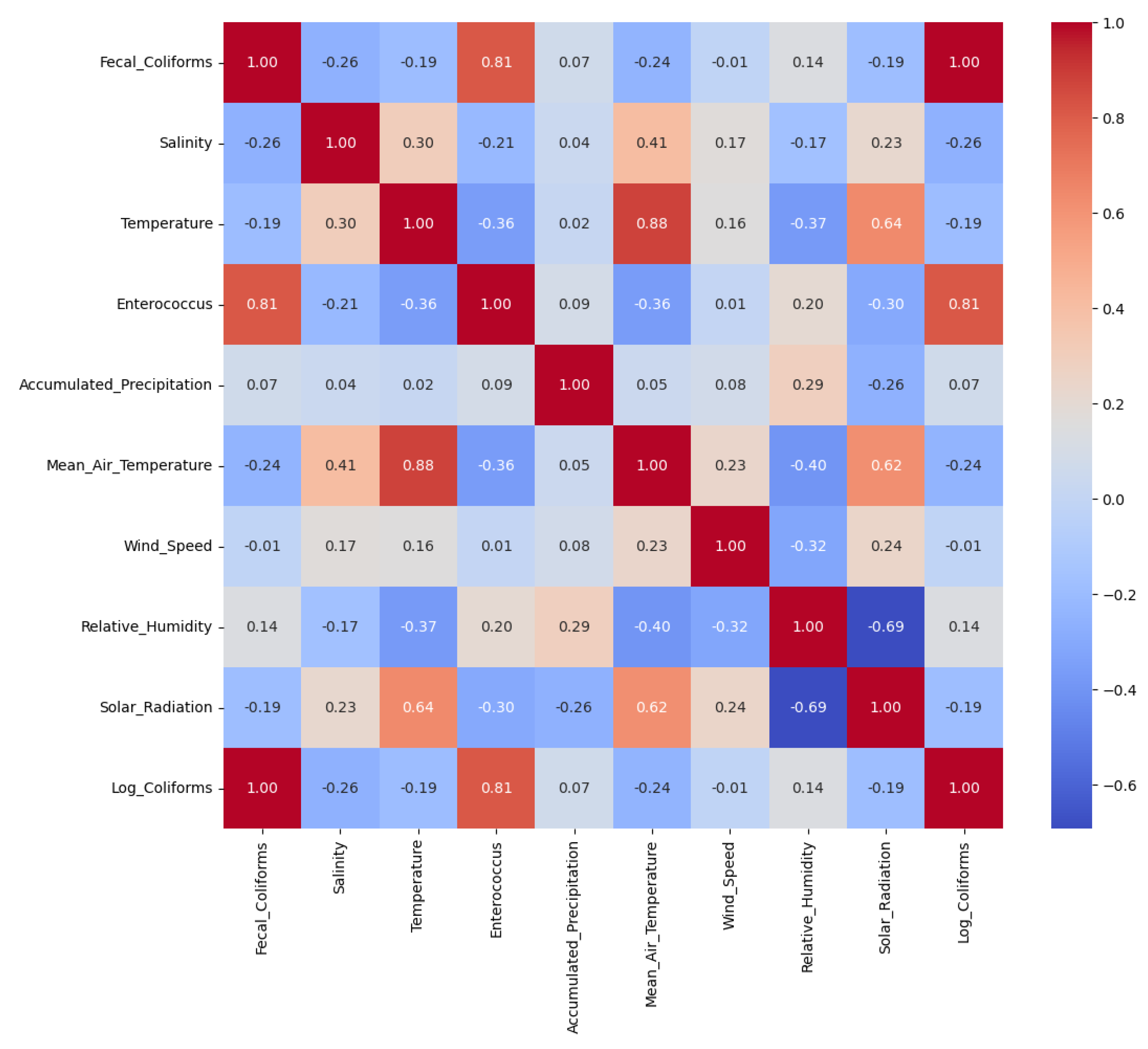
To explore relationships between variables, we computed both Spearman and Kendall rank correlation coefficients. Since the results were highly similar, we present only the Spearman correlation matrix for simplicity (Figure 5). A strong positive correlation was observed between fecal coliforms and enterococcus (Spearman = 0.813; Kendall = 0.631), which is expected as both are fecal indicator bacteria commonly used to assess microbiological water quality. Their simultaneous increase typically reflects contamination from a shared source, such as combined sewer overflows or stormwater discharges carrying human or animal waste. Another noteworthy correlation was found between water and air temperatures (Spearman = 0.881; Kendall = 0.701). This is also consistent with physical expectations, as water temperature responds to atmospheric conditions. Warmer air temperatures tend to result in higher water temperatures, especially in shallow coastal environments, due to heat exchange and solar radiation. In addition, both air temperature and water temperature showed moderate to strong positive correlations with solar radiation (Spearman = 0.617 and 0.639, respectively). This is consistent with the expected energy balance dynamics, where increased solar radiation leads to surface warming of both air and water bodies. Conversely, a strong negative correlation was found between relative humidity and solar radiation (Spearman = −0.692), which can be explained by the typical inverse relationship between sunlight and moisture: sunnier conditions often coincide with drier air, especially during the daytime when solar radiation is at its peak.

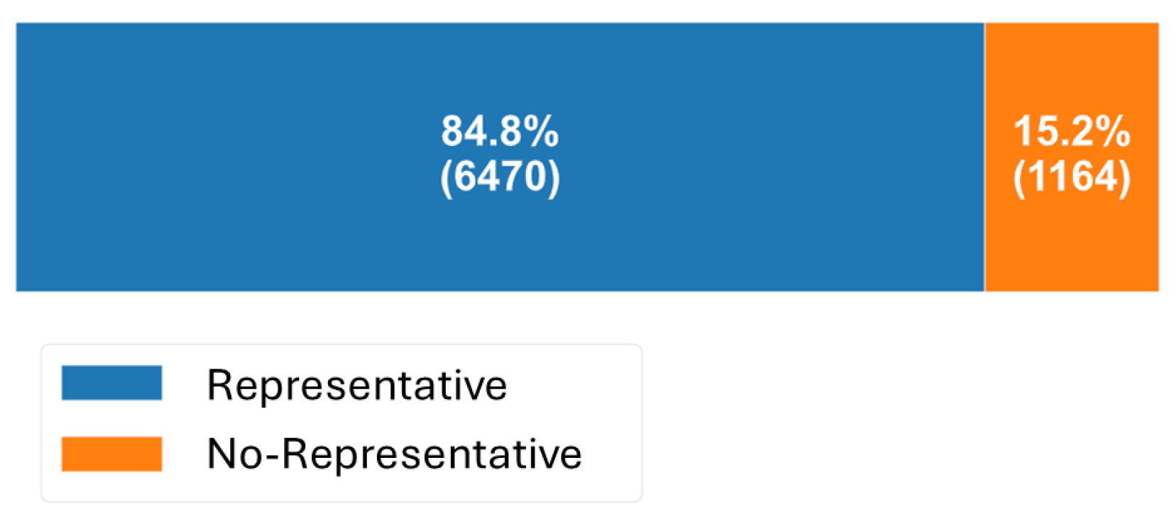
Regarding sample representativeness, 84.8% of the water quality measurements were labeled as Representative, indicating that no rainfall-induced discharges occurred within the 24 h prior to sampling. In contrast, only 15.2% of the samples were classified as No Representative, meaning they were collected following rainfall events, potentially capturing conditions affected by combined sewer overflows or stormwater runoff (Figure 6). This distribution supports the predominance of routine monitoring under dry-weather conditions, while also highlighting the limited but relevant influence of wet-weather events on water quality.

3.2. Hyperparameter Optimization

Table 5. Best hyperparameters for each optimized regression model.

Model	Best Hyperparameters
SVR	C = 13.44, gamma = auto, kernel = rbf, epsilon = 0.485
DTR	max_depth = 6, min_samples_split = 13, min_samples_leaf = 18, criterion = poisson
RFR	n_estimators = 343, max_depth = 23, min_samples_split = 12,
	min_samples_leaf = 1, max_features = log2
HGBR	learning_rate = 0.016, max_iter = 497, max_leaf_nodes = 34,
	max_depth = 4, l2_regularization = 6.65 $\times {10}^{-6}$

summarizes the optimal hyperparameter configurations obtained for each regression model after tuning, highlighting the diversity in complexity and regularization strategies selected for different algorithms.

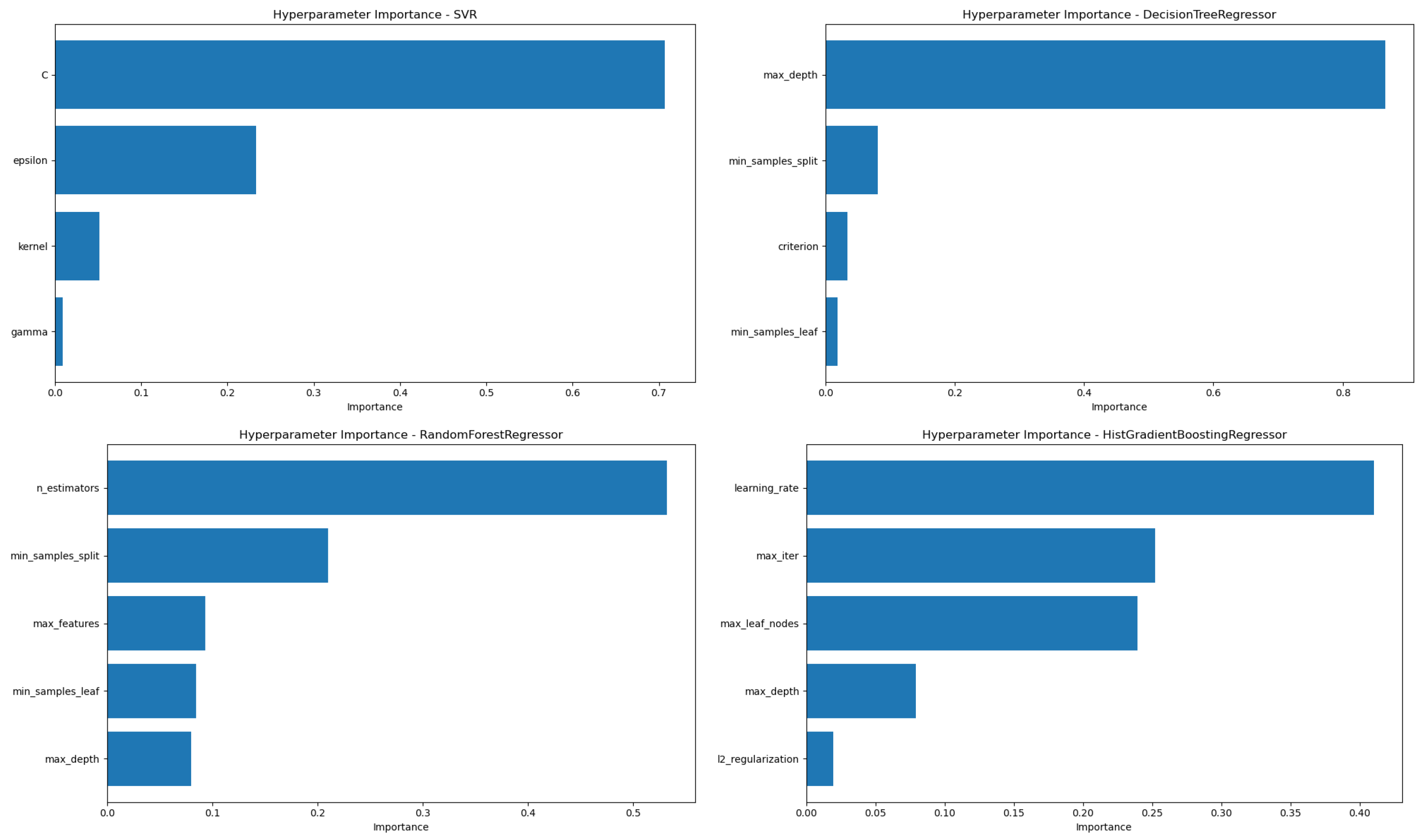
Subsequently, we evaluated the importance of each hyperparameter to better understand which parameters most significantly influenced model performance during the optimization process (Figure 7).

The analysis of hyperparameter importance revealed distinct patterns across models, reflecting the differing mechanisms by which each algorithm controls complexity and generalization. For the Support Vector Regressor (SVR), the regularization parameter C emerged as the most influential hyperparameter, significantly affecting model flexibility and the trade-off between bias and variance. The second most important was $epsilon$, which defines the width of the margin within which no penalty is given for errors, highlighting its role in controlling model tolerance to deviations. In the case of the Decision Tree Regressor (DT), the tree depth ($max\text{\_}depth$) has a significant impact on model performance, which aligns with its direct effect on model complexity and control of overfitting. For the Random Forest (RF) model, the number of estimators ($n\text{\_}estimators$) had the most significant influence, likely because ensemble performance strongly depends on the number of trees used. Interestingly, $min\text{\_}samples\text{\_}split$ was more important than $max\text{\_}depth$, which had the least influence—perhaps due to sufficient depth being achieved early across trees, reducing the marginal gain of increasing depth further. Finally, in the HistGradient Boosting Regressor (HGB), $learning\text{\_}rate$ proved to be the most critical, as it governs the contribution of each boosting step and thus heavily affects convergence. This was followed by $max\text{\_}iter$ and $max\text{\_}leaf\text{\_}nodes$, both of which influence the model’s capacity to learn complex relationships while mitigating overfitting. These results highlight the importance of tuning model-specific parameters that most directly shape the learning dynamics and structural capacity of each algorithm.

3.3. Model Performance Evaluation

To evaluate the predictive capacity of different algorithms, five regression models were trained and tested using Log-transformed fecal coliform concentrations as the target variable.

Table 6. Model performance metrics for training and test datasets and their uncertainty.

Model	Dataset	MSE	NSE	PBIAS (%)	Uncertainty
Linear Regression (baseline)	Train	0.45	0.15	−0.00
	Test	0.49	0.08	−1.49	0.034
Support Vector Regressor	Train	0.43	0.18	0.02
	Test	0.48	0.10	−1.27	0.064
Decision Tree Regressor	Train	0.16	0.70	0.00
	Test	0.17	0.67	−0.63	0.129
Random Forest Regressor	Train	0.07	0.87	−0.04
	Test	0.16	0.70	−0.83	0.068
HistGradient Boosting Regressor	Train	0.14	0.74	0.00
	Test	0.16	0.70	−0.56	0.568

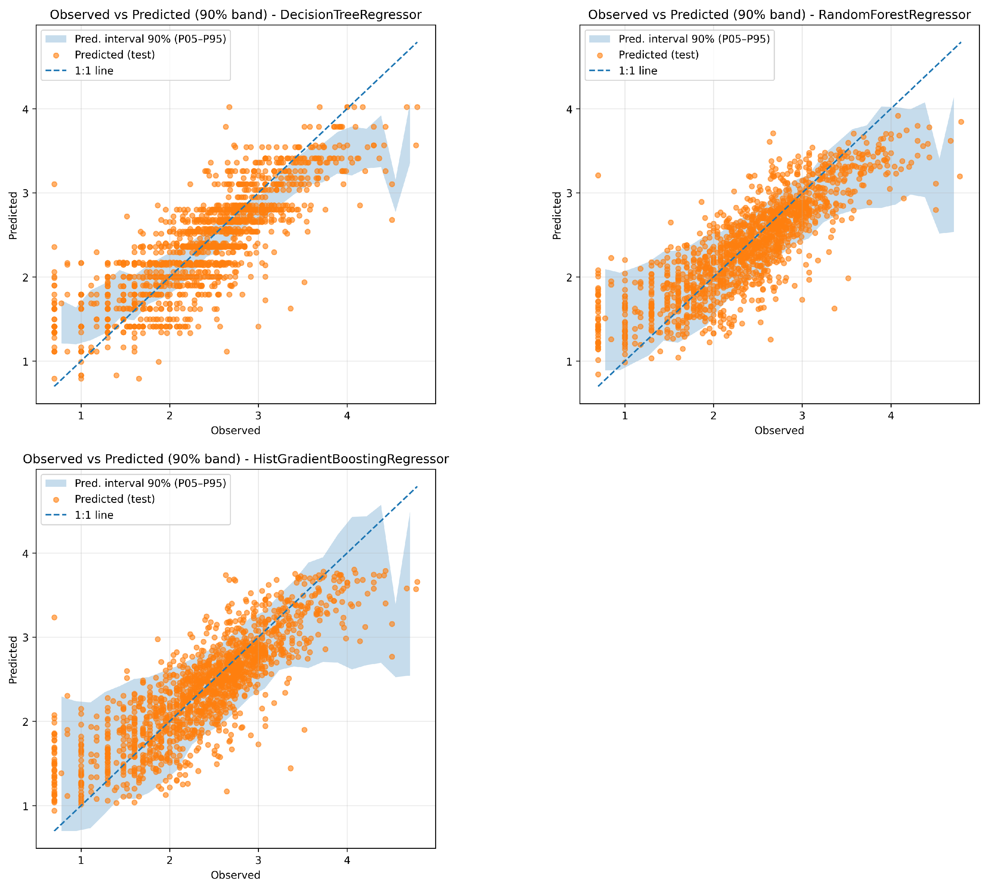
summarizes the performance of each model across the training and test datasets, using MSE, NSE, and PBIAS as evaluation metrics. Figure 8 shows the scatter plots of observations vs. predictions for the three best models (Decision Tree, Random Forest, and HistGradient Boosting), including the corresponding 90% prediction intervals to illustrate model uncertainty.

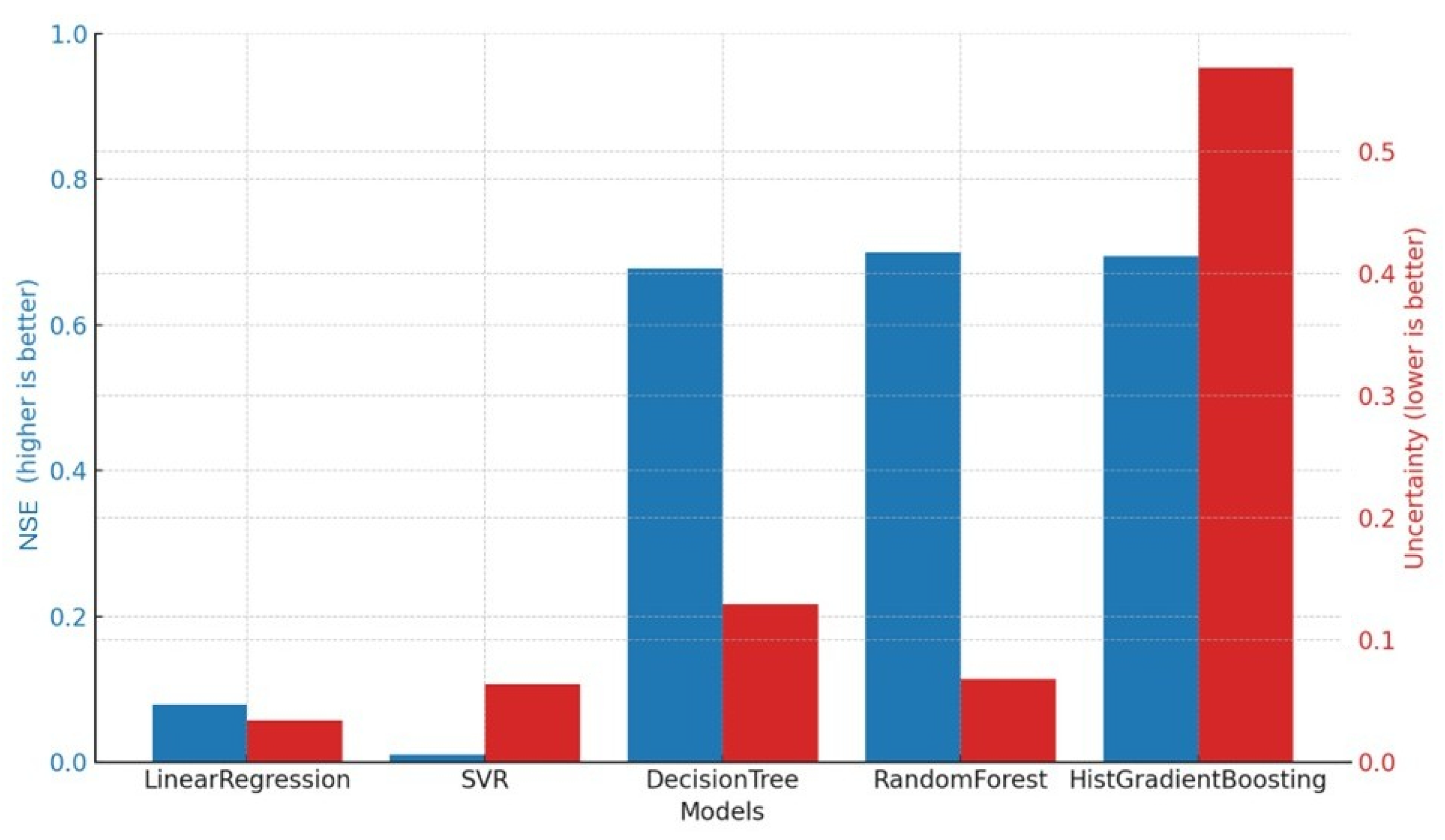
The Linear Regression model, used as a baseline, showed limited predictive capability, with low NSE values on both the training (0.15) and test set (0.08). Although its PBIAS values were close to zero, indicating an overall unbiased prediction, the high MSE reflects its inability to capture the non-linearities and variance in the data. The uncertainty was low, but this was a consequence of the model’s rigidity and underfitting rather than genuine predictive reliability.

The Support Vector Regressor improved upon the baseline slightly, with higher NSE values (0.18 on the training set and 0.10 on the test set) and lower MSE. SVR’s ability to capture some non-linear patterns led to more accurate and stable predictions, although the performance gain was still modest. The uncertainty levels were moderate, but given the poor performance, this did not translate into meaningful reliability.

The Decision Tree Regressor showed a good fit on the training data (NSE = 0.70, MSE = 0.16), with only a slight drop in performance on the test set (NSE = 0.67), indicating that the model generalized reasonably well. While its training performance was higher, the small performance gap suggests only mild overfitting. However, the uncertainty associated with this model was higher than other ensemble methods, reflecting its sensitivity to data fluctuations and the inherent instability of single-tree models.

The Random Forest Regressor achieved an NSE of 0.87 on the training set and 0.70 on the test set, it delivered the highest predictive power and lowest MSE among all models, while maintaining very low bias. Importantly, its uncertainty was also among the lowest, indicating robust and stable predictions. This demonstrates the benefit of ensemble averaging in reducing variance and overfitting, while retaining high accuracy.

The HistGradient Boosting Regressor also showed strong predictive performance, with NSE values of 0.74 and 0.70 for the training and test sets, respectively, and the lowest test MSE of 0.16. Its bias was the lowest of all models, suggesting well-centered predictions. However, its predictive uncertainty was substantially higher than that of the other ensemble method, raising concerns about the stability and reliability of its forecasts, despite the good average metrics. This suggests that while gradient boosting can effectively capture complex interactions and high-order non-linearities, it may be more sensitive to data variability in practice.

Overall, ensemble-based methods outperformed both the linear and kernel-based alternatives. Among them, Random Forest provided the most reliable balance between accuracy and uncertainty, making it the most robust choice for predicting fecal contamination levels. While HistGradient Boosting achieved comparable accuracy, its elevated uncertainty highlights the need for caution in its application. These findings reinforce the adoption of tree-based ensemble models, particularly Random Forest, as effective and dependable tools for handling skewed and heterogeneous environmental datasets.

In Figure 9, a comparison of model performance and uncertainty is reported.

3.4. Most Influential Features for Coliform Prediction

To gain insights into the internal reasoning of the best-performing model, a SHAP analysis was conducted on the Random Forest (Figure 10). This model not only achieved the highest predictive performance but also demonstrated the ability to capture key physical and biogeochemical processes influencing fecal coliform concentrations. It is worth noting that the SHAP analysis results were highly consistent across all three tree-based models (Decision Tree, Random Forest, and HistGradient Boosting), reinforcing the robustness of the identified key drivers.

The SHAP summary plot (Figure 10) shows that enterococcus was the most influential feature by a large margin, dominating the model’s predictions. This is consistent with expectations, as both indicators originate from similar sources of fecal contamination and tend to covary, particularly under high-load conditions. The high SHAP values associated with enterococcus reflect its strong and consistent contribution to predicting fecal coliform levels.

Salinity emerged as the second most important predictor. Its relevance can be attributed to the fact that freshwater inflows tend to dilute both salinity and fecal contaminants. Lower salinity values often correspond to stormwater events or increased runoff, which are also associated with spikes in microbial concentrations. The model successfully captured this inverse relationship.

Water temperature ranked third in importance, likely due to its influence on microbial survival, metabolic activity, and decay rates. Higher temperatures can promote bacterial growth up to a certain point, and their strong correlation with other environmental variables (e.g., solar radiation, seasonality) further supports their predictive relevance.

Interestingly, accumulated precipitation ranked as the least influential variable in the SHAP analysis. This result is somewhat unexpected, given the known role of rainfall in mobilizing fecal contaminants through surface runoff and combined sewer overflows. One possible explanation is that the precipitation monitoring station used in this study is located too far from the coastal sampling sites, and therefore may not accurately capture the localized rainfall events that influence water quality near the shoreline. Additionally, the temporal mismatch between rainfall events and sampling times, especially if peak contamination occurs shortly after rainfall and is not consistently captured during regular sampling, could reduce the apparent influence of precipitation in the model. These limitations underscore the need to enhance the spatial and temporal resolution of rainfall data for future studies.

Figure 11 shows the SHAP interaction plot for enterococcus and salinity, the two most influential predictors identified in the RF model. This plot effectively reveals the relationship between enterococcus concentration and salinity in predicting fecal coliform levels. While high enterococcus concentrations consistently result in the highest positive SHAP values, indicating it’s the dominant predictor of high contamination regardless of salinity, the plot highlights a critical conditional risk factor at lower microbial levels. Specifically, when enterococcus concentrations are low, the model’s prediction is strongly influenced by salinity: the presence of low salinity (blue points) significantly amplifies the positive impact of even moderate enterococcus readings (pushing the SHAP value higher). Conversely, a high salinity (red points) reinforces the model’s prediction of a low coliform risk when enterococcus is low, driving the SHAP value to be more negative. This pattern supports the hypothesis that low salinity acts as a crucial contextual proxy for freshwater runoff and dilution, maximizing the predicted risk associated with microbial indicators following a contamination event.

4. Discussion

The Log-transformed boxplot of thermotolerant coliforms reveals meaningful differences in microbial water quality across Montevideo’s beaches. To quantitatively contextualize these values, we compare the observed concentrations with the bathing water quality standards defined by the Ministry of Environment of Uruguay (Ministerio de Ambiente) [30] (

Table 7. Percentage of samples exceeding thermotolerant coliform thresholds at selected beaches.

Beach	>1000 CFU/100 mL (%)	>2000 CFU/100 mL (%)
Del Cerro	25.0	14.0
Ramirez	22.6	11.8
Pocitos	14.1	5.4
Carrasco	16.5	7.7
Malvin	13.9	6.5
Pajas Blancas	4.1	1.9

).

Beaches such as Del Cerro and Ramirez exhibit notably elevated bacterial concentrations, with around 25% and 22.6% of samples, respectively, exceeding the 1000 CFU/100 mL threshold. More alarmingly, roughly 14% and 11.8% of samples at these locations surpass 2000 CFU/100 mL, suggesting recurring health risks for recreational users.

By contrast, beaches like Malvin, Pocitos, and Carrasco show more moderate levels, though still with 13–16% of samples exceeding the 1000 CFU/100 mL mark. Pajas Blancas consistently demonstrates the best microbial quality among the group, with only 4.1% of samples above 1000 CFU/100 mL and fewer than 2% above 2000.

The EDA revealed a high correlation between enterococci and thermotolerant coliforms, a result that aligns with their common fecal origin and similar environmental behavior. This strong association was further confirmed in the SHAP analysis, where enterococci emerged as the most influential variable in the model predicting coliform concentrations, with an order of magnitude greater importance compared to the following most relevant variable, salinity. This dominance is expected given the shared sources of contamination and the persistence patterns of both bacterial indicators in coastal environments.

Salinity and water temperature ranked similarly in the SHAP analysis, with comparable influence, supporting previous findings in the literature. For instance, Segura et al. [16] identified salinity as one of the most influential predictors of fecal coliform concentrations, while Bourel et al. [19] found that fecal coliform classification depends on salinity and water temperature. These physicochemical parameters are known to capture the local dynamics of beach and watershed interactions, and are particularly relevant in coastal urban settings where tidal movements, freshwater discharges, and ambient conditions interact closely.

The seasonality observed in the distribution of thermotolerant coliforms can be primarily attributed to the influence of water temperature, which is closely linked to air temperature [31]. During the summer months, elevated air temperatures result in higher water temperatures, creating more favorable conditions for bacterial growth and persistence [15]. Conversely, in winter, lower temperatures can inhibit microbial activity and promote faster decay rates. This seasonal pattern was reflected in both the EDA and the correlation analysis, where a moderate positive correlation was found between coliforms and water temperature. This relationship directly influences model predictions, as temperature-related features were consistently among the most influential predictors identified by the SHAP analysis (Figure 10), reinforcing the model’s ability to capture temperature-driven variability in contamination levels. Moreover, this seasonal behavior aligns with the typical hydrometeorological dynamics of the Río de la Plata estuary, where warmer summer conditions and reduced freshwater dilution favor microbial persistence, while winter mixing and lower temperatures lead to decreased concentrations [32,33].

The limited predictive power of accumulated precipitation in our model may be attributed to a combination of spatial, temporal, and representativeness limitations.

• First, the rainfall data used were collected from a monitoring station that is not located in the immediate vicinity of the coastal sampling sites. This spatial mismatch can lead to non-representative precipitation values, particularly in regions where rainfall events are highly localized and concentrated.
• Second, there is often a temporal lag between rainfall and the observed increase in fecal contamination, as runoff takes time to travel through the watershed and transport fecal coliforms and other pollutants into the water bodies [34]. If water samples are not collected at intervals that align with these post-rainfall runoff dynamics, the relationship between precipitation and contamination may be obscured. This was also confirmed by Suh et al. [15].
• Third, only a limited number of the samples in our dataset correspond to periods shortly after rainfall events. As a result, the model may be trained mostly on “dry-weather” data (84.8% of the data), where precipitation is not a relevant driver (Representative samples), thus diminishing its overall importance in the feature ranking.

These factors together help explain why accumulated precipitation appeared as the least influential variable in the SHAP (Figure 10), despite its known relevance in the transport of fecal pollutants.

Building on these variable-specific insights, the overall model performance, our results showed that both Random Forest and Histogram-based Gradient Boosting achieved very good performance according to the evaluation criteria proposed by Moriasi et al. [28]. These models demonstrated strong predictive capabilities, with high coefficients of determination and low error metrics, reflecting their effectiveness in capturing the variability of fecal coliform concentrations. However, when predictive uncertainty was considered, Random Forest provided the most reliable balance between accuracy and stability, whereas Histogram-based Gradient Boosting, despite achieving comparable accuracy, exhibited substantially higher uncertainty. This highlights the advantage of Random Forest as a robust choice for environmental datasets, where stability and reliability are critical in addition to predictive accuracy. These results are consistent with previous local studies, such as those by Crisci et al. [35] and Bourel et al. [18], which also found that Random Forest and Boosting models were the most effective algorithms for predicting microbiological water quality. The convergence of these findings reinforces the robustness of ensemble learning methods for modeling fecal contamination in coastal and urban water systems.

When compared to other recent studies, our models demonstrate competitive performance. For example, Suh et al. [15] applied various machine learning models, including XGBoost and Convolutional Neural Networks, to predict fecal coliform concentrations in four major South Korean rivers. Their best-performing model, XGBoost, achieved a validation NSE of 0.597 in the Han River, which is notably lower than the test NSE of 0.70 achieved by both our Random Forest and Histogram-based Gradient Boosting models. While their study benefited from a rich dataset spanning eight years and multiple water quality variables, their relatively lower predictive performance highlights the challenge of modeling microbial indicators under diverse hydrological conditions. Similarly, Hannan and Anmala [13] applied Random Forest to predict microbial contamination in surface waters in the U.S. and reported validation R² values generally ranging from 0.45 to 0.65 depending on the site and indicators. Though not directly comparable to NSE, these metrics suggest moderate predictive performance, again underscoring the difficulty of generalizing across sites and indicator types.

In contrast, Sbahi et al. [10] investigated fecal coliform removal from wastewater using three ML algorithms (ANN, Cubist, and MLR) in controlled laboratory-scale systems. Their best-performing model (ANN) achieved an R² of 0.953, substantially higher than ours. However, this difference largely reflects the controlled and homogeneous nature of their dataset, which minimizes environmental variability and measurement noise. In real-world, field-based applications such as ours, characterized by fluctuating hydrological, meteorological, and anthropogenic drivers, achieving an NSE of 0.70 represents a strong predictive capability. Our results, therefore, illustrate the robustness of the models under realistic operational conditions, where data uncertainty and spatial heterogeneity typically limit performance.

Overall, our models show comparable or superior skill to other recent studies when accounting for data complexity and study design (

Table 8. Comparison of model performance for fecal coliform prediction across recent studies.

Study	Context	ML Models Used	Data Type/Setting	Performance Metric	Value
Suh et al. [15]	Major rivers in South Korea	XGBoost, CNN	Field, multi-year dataset	NSE (validation)	0.597
Hannan and Anmala [13]	Surface waters, USA	Random Forest	Field, site-specific	R2 (validation)	0.45–0.65
Sbahi et al. [10]	Wastewater, lab-scale	ANN, Cubist, MLR	Controlled laboratory	R2 (validation)	0.953
This study (2025)	Urban coastal system, Uruguay	Random Forest, HGB	Field, variable hydrological regime	NSE (test)	0.70

), confirming their potential for practical applications in urban water quality assessment.

5. Practical Value of the Findings

From an operational and economic perspective, developing a predictive model for fecal coliform concentrations is both practical and cost-effective. Given that the laboratory methods for enumerating fecal coliforms (APHA 9222 D [36]) and enterococci (EPA Method 1600 [37]) involve similar membrane filtration procedures, require comparable levels of technical expertise, and rely on analogously priced consumables and equipment, the overall effort for monitoring either indicator is equivalent.

However, when both indicators are monitored in parallel, as currently done in Montevideo, this effectively doubles the required laboratory effort, from sample processing to incubation and enumeration. Each analysis involves separate media, incubation conditions, and quality control. In this context, deploying a reliable predictive model allows environmental agencies to reduce analytical redundancy. If enterococci are already being measured, as they are part of routine monitoring, a robust model can estimate fecal coliform concentrations without incurring the additional time and cost of performing a second analysis.

Beyond operational efficiency, predicting continuous fecal coliform concentrations provides substantial advantages over traditional classification approaches that rely solely on regulatory thresholds. Continuous predictions enable the detection of subtle trends and emerging risks, support real-time decision-making, and allow for flexible management strategies based on risk gradients rather than binary outcomes. This is particularly useful in managing beach advisories, where microbial levels often fluctuate near regulatory thresholds, and more nuanced information can support more responsive and adaptive public health decisions. In addition, this modeling framework provides a foundation for integration with real-time data sources such as IoT-based monitoring stations or remote-sensing products, paving the way for operational early warning systems. The models could also be embedded within decision-support platforms for municipal beach management, facilitating proactive and data-driven interventions that enhance public health protection.

In addition, this approach enables the extension of fecal coliform predictions to periods and locations where direct measurements are not available, helping to fill spatiotemporal gaps in monitoring and providing timely information for more adaptive beach management.

Furthermore, while our discussion has focused on the application of this predictive framework in Montevideo, the portability of our modeling approach should not be overlooked. Because it leverages widely available environmental and microbial data, the methodology could be adapted for use in other urban coastal settings. Additionally, our use of open-access meteorological and water quality datasets, along with transparent code and reproducible workflows, supports broader implementation by environmental managers and researchers.

Nevertheless, several limitations must be acknowledged. One primary challenge relates to the precipitation data used: rainfall measurements were obtained from a station several kilometers away from the sampling sites, potentially failing to capture localized rainfall variability that drives contamination. Although the present study focused on model development using a pooled dataset to ensure sufficient data density across beaches, future work will include external validation schemes, such as leave-one-beach-out cross-validation, to explicitly test spatial transferability and model robustness. Additionally, the temporal resolution of the meteorological and water quality data, primarily daily measurements, may be insufficient to detect rapid water quality changes that occur at sub-daily scales, such as immediate runoff impacts following short but intense rainfall events. The lag time between rainfall and sampling, combined with relatively few samples collected shortly after rain events, further restricts the model’s capacity to predict contamination peaks associated with storm-driven runoff.

Moreover, while the model includes commonly measured environmental variables, important drivers such as land use dynamics, hydrodynamic conditions, point-source pollution events, or microbial die-off rates were not explicitly considered. This omission may limit the explanatory power and predictive accuracy of the models, especially under changing environmental conditions. In addition, the study did not extensively quantify model uncertainty, which constrains the ability to assess the confidence or reliability of predictions, particularly under rare or atypical conditions such as extreme weather events or accidental discharges.

6. Conclusions

This study demonstrated the potential of machine learning (ML) approaches for predicting fecal coliform concentrations in urban coastal environments, using Montevideo’s beaches as a case study. Among the tested models, Random Forest achieved the best performance, with test NSE values around 0.70, reflecting robust generalization and high predictive accuracy. SHAP analysis revealed enterococci as the most influential predictor, underscoring their complementary role in describing microbial contamination pathways, followed by water temperature and salinity, which capture seasonal and hydrodynamic variability typical of the Río de la Plata estuary.

Our three main objectives were successfully addressed:

1.

We developed and validated ML models that provide continuous fecal coliform estimates rather than binary classifications, effectively capturing non-linear relationships among environmental variables.

2.

We demonstrated the practical value of these models for water quality management: they enable timely, cost-effective estimation of fecal contamination levels, potentially reducing the need for redundant laboratory analyses when enterococci are already monitored, and supporting more responsive beach advisories based on continuous risk levels.

3.

By assessing feature importance using SHAP, we identified key environmental drivers (enterococci, temperature, and salinity), providing new insight into the processes governing microbial dynamics in estuarine waters.

From an operational perspective, these findings highlight the feasibility of integrating ML models into existing monitoring frameworks to enhance predictive capacity and resource efficiency. As discussed in Section 5 (“Practical Value of the Findings”), this approach can inform more adaptive and data-driven coastal management strategies in Montevideo and similar urban coastal systems.

While the models performed well, several limitations remain. These include the coarse spatial and temporal resolution of the input data, the limited number of samples following rainfall events, and the absence of dynamic predictors such as tidal influence, land-use changes, and microbial decay rates. Addressing these limitations in future work, through denser monitoring networks, higher-frequency data collection, and integration of real-time datasets, will further strengthen model reliability and applicability for early-warning systems.

In summary, this study demonstrates that integrated, interpretable ML approaches can provide both accurate predictions and actionable environmental insights, contributing to more efficient microbial water quality management. Nonetheless, their generalization to other settings should be pursued cautiously, supported by site-specific data and validation.