A Spectral Analysis-Driven SARIMAX Framework with Fourier Terms for Monthly Dust Concentration Forecasting

Abstract

This study aimed to forecast monthly PM_2.5 concentrations in Zabol, one of the world’s most dust-prone regions, using four time series models: SARIMA, SARIMAX enhanced with Fourier terms (selected based on spectral peak analysis), TBATS, and a novel hybrid ensemble. Spectral analysis identified a dominant annual cycle (frequency 0.083), which justified the inclusion of two Fourier harmonics in the SARIMAX model. Results demonstrated that the hybrid model, which optimally combined forecasts from the three individual models (with weights ω₂ = 0.628 for SARIMAX, ω₃ = 0.263 for TBATS, and ω₁ = 0.109 for SARIMA), outperformed all others across all evaluation metrics, achieving the lowest AIC (1835.04), BIC (1842.08), RMSE (9.42 μg/m³), and MAE (7.43 μg/m³). It was also the only model exhibiting no significant residual autocorrelation (Ljung–Box p-value = 0.882). Forecast uncertainty bands were constant across the prediction horizon, with widths of approximately ±11.39 μg/m³ for the 80% confidence interval and ±22.25 μg/m³ for the 95% confidence interval, reflecting fixed absolute uncertainty in the multi-step forecasts. The proposed hybrid framework provides a robust foundation for early warning systems and public health management in dust-affected arid regions.

1. Introduction

Ambient air pollution, particularly elevated levels of fine particulate matter (PM_2.5 and PM₁₀), poses a significant threat to environmental sustainability and public health worldwide. Prolonged exposure to PM_2.5 is strongly linked to higher rates of cardiovascular and respiratory morbidity and mortality [1]. In arid and semi-arid regions, frequent dust storms further degrade air quality and amplify the health risks associated with fine particulate matter [2]. With millions of people residing in dust-prone zones across the Middle East and Central Asia, protecting public health requires timely and accurate forecasting of airborne dust concentrations [3]. In this regional context, operational dust-forecasting capabilities are critical for risk mitigation and environmental management [4].

Despite significant advancements in atmospheric monitoring, operational forecasting of dust concentrations remains a complex challenge due to the nonlinear behavior and pronounced temporal variability of particulate matter. Persistent dust events and fluctuating pollutant loads in arid and urban regions demand robust predictive tools [5]. Classical time series models such as ARIMA (Autoregressive Integrated Moving Average) and SARIMA (Seasonal Autoregressive Integrated Moving Average) have been widely utilized to forecast environmental variables, including solar radiation [6], temperature [7], and both PM_2.5 and PM₁₀ concentrations [8,9,10]. These models are generally well-suited for capturing short-term trends and seasonal cycles in air quality data, requiring limited input parameters and enabling computational efficiency [11,12]. Nevertheless, they often fail to fully capture persistent or deterministic seasonal patterns, particularly when complex cyclic components exist in the data, as evidenced by residual autocorrelation at seasonal lags, which can compromise forecast reliability [13].

To address these limitations, extensions such as SARIMAX models—by incorporating exogenous regressors (e.g., meteorological variables, calendar/seasonal indicators, or lagged external indices)—can better capture systematic cyclic behavior and thereby improve forecast performance [7,11].

Models like TBATS (Box–Cox transformation, ARMA errors, Trend, and Seasonal components). further expand this capability by accommodating multiple or non-integer seasonality, making them attractive for complex time series [14]. However, even these flexible models may be limited in spatial generalization and can underperform during rapid, non-stationary changes such as extreme dust events or abrupt meteorological shifts [15,16].

Recent research has thus shifted toward hybrid approaches, integrating external regressors, spectral decomposition, or nonlinear machine learning techniques to overcome the limitations of classical statistical models [9,17,18]. For example, Doreswamy et al. [12] and Díaz-Robles et al. [19] have shown that ARIMA-based hybrid frameworks with machine learning components can effectively capture both linear and nonlinear dependencies in PM_2.5 and PM₁₀ data. The widespread use of SARIMA and SARIMAX for air quality prediction has been documented in various regions [20,21], but these models often struggle to capture persistent deterministic and recurring seasonal cycles fully. To address this limitation, spectral decomposition techniques, such as the inclusion of Fourier terms in SARIMAX, have been increasingly adopted [11,22].

Recent studies further confirm the value of SARIMAX–Fourier formulations for environmental applications: Necula et al. [23] integrated Fourier-based SARIMAX within hybrid pollution-forecasting frameworks, Avila et al. [24] demonstrated its effectiveness for multi-seasonal environmental series. These contributions underscore the growing relevance of SARIMAX–Fourier models for environmental and air-quality forecasting.

Recent advances in air quality forecasting have demonstrated the high effectiveness of hybrid modeling approaches for predicting PM_2.5 concentrations, particularly in complex urban environments. By combining statistical models like ARIMA and SARIMA with advanced machine learning and deep learning methods, including BiLSTM, SALSTM, LSSVM, and ANN, researchers have achieved notable improvements in predictive accuracy. These hybrids leverage both linear and nonlinear modeling strengths, capturing intricate temporal patterns in pollutant data [23,25,26]. For example, Du et al. [25] showed substantial gains with a SARIMA–deep learning hybrid, while Albeladi et al. [26] highlighted the effectiveness of LSTM–ARIMA integration. Incorporating spatial features, as Liu et al. [27] did for Wuhan, further enhances accuracy in highly variable pollution settings. Necula et al. [23] developed a SARIMA–BiLSTM hybrid, achieving robust results, and Solis Teran et al. [28] confirmed the operational value of hybrid frameworks in Lima, Peru.

Complementing these methods, the TBATS model represents a major advancement for forecasting time series with complex or non-integer seasonality, such as those found in environmental applications. TBATS utilizes trigonometric terms within its exponential smoothing framework to flexibly model overlapping or evolving seasonality [14,29,30]. Naim et al. [29] and Andreozzi et al. [30] showed that TBATS outperforms traditional approaches, particularly in multi-seasonal contexts. Such hybrid approaches highlight the importance of combining linear and nonlinear modeling strategies, informed by the nature of the data, to achieve accurate forecasts in hydrological and environmental applications [18,19]. Together, these approaches illustrate the importance of combining statistical rigor with domain knowledge and spectral diagnostics to develop robust forecasting tools for environmental health applications.

Despite substantial progress in time series modeling for air quality forecasting, notable research gaps persist, particularly in arid regions such as Zabol in southeastern Iran, where dust dynamics are exceptionally complex and environmental extremes are intensified by the desiccation of the Hamoun wetlands. Zabol has become internationally recognized for its frequent and severe dust storms, with annual PM_2.5 and PM₁₀ concentrations regularly surpassing both national and global air quality standards. The region’s characteristic “120-day wind” phenomenon, driven by hyper-arid climatic conditions, results in recurrent, acute dust episodes that substantially elevate risks of respiratory and cardiovascular diseases among the local population [31,32,33,34,35].

While several classical time series models have been applied to air quality forecasting, there is a notable lack of studies systematically evaluating advanced hybrid models, particularly those integrating spectral analysis and deterministic seasonal components, for dust prediction in such challenging environments. Addressing this gap, the present study develops and assesses a SARIMAX model augmented with Fourier terms, guided by spectral diagnostics, for monthly PM_2.5 forecasting in Zabol. By comparing this approach with traditional SARIMA and TBATS models, the research aims to offer both methodological advancement and actionable insights to support early warning systems and dust management strategies in one of the world’s most severely dust-affected regions.

2. Study Area and Datasets

Zabol, situated in southeastern Iran, is widely documented as a wind-exposed, dust-prone area within the Sistan Basin [32,33,36]. The area’s hyper-arid climate and low annual precipitation, combined with the progressive desiccation of the Hamoun wetlands, have dramatically increased the frequency and severity of dust storms in recent decades [37,38]. This process has been further exacerbated by recurring droughts, significant land use changes such as agricultural expansion and upstream water diversion, all of which have accelerated wetland loss and intensified dust emission events, leading to pronounced seasonality in particulate pollution [37]. Zabol is strongly affected by the “120-day wind” (Levar), a persistent summer wind system that transports large volumes of mineral dust from the desiccated Hamoun basin into urban and rural environments [33]. These conditions, together with the region’s flat and sparsely vegetated topography, create optimal circumstances for dust mobilization and atmospheric transport [32].

Zabol has been reported to exhibit elevated annual average PM_2.5 and PM₁₀ levels in Iran [31]. Given these unique climatic and geographical features, Zabol represents an ideal natural laboratory for investigating the dynamics of particulate matter pollution and the performance of advanced forecasting models in extreme dust conditions. 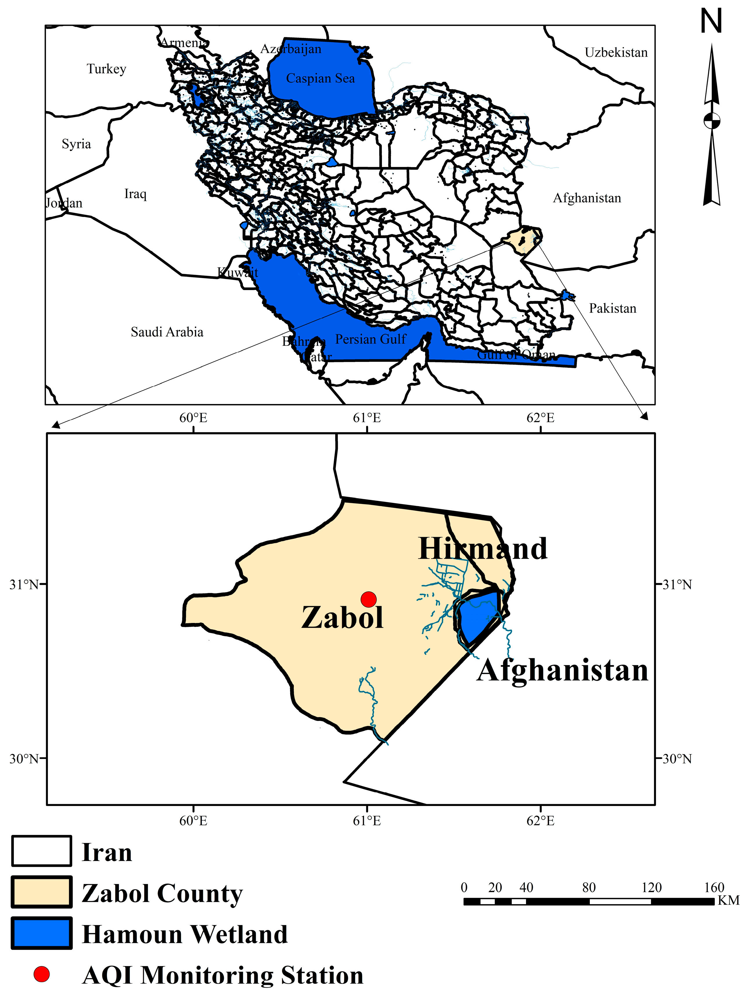For this study, a monthly time series dataset of fine particulate matter (PM_2.5; aerodynamic diameter < 2.5 µm) was collected from the primary air quality monitoring station in Zabol. The dataset spans 21 years from 2004 to 2025, yielding 264 monthly observations from government-operated environmental monitoring stations. The geographical location of Zabol and the monitoring site is illustrated in Figure 1.

3. Methodology

This study aims to develop a reliable and interpretable framework for forecasting monthly concentrations of fine particulate matter (PM_2.5) in Zabol. The research applies and compares four time series modeling approaches: the classical Seasonal ARIMA (SARIMA) model, the TBATS model, and a modified SARIMAX model augmented with Fourier terms and a hybrid model. The methodology consists of a sequence of analytical stages and a comparative evaluation of model performance based on information criteria and forecast accuracy metrics. All computations and visualizations were performed in R (v4.4.2) using the forecast, stats, and ggplot2 packages.

3.1. Exploratory Data Analysis and Stationarity Assessment

An essential first step in time series modeling is to evaluate the statistical characteristics and stationarity of the data, particularly for ARIMA-based approaches [13]. Exploratory data analysis involved visualizing the time series to identify recurring seasonal patterns and any long-term trends, which are important for determining the suitability of seasonal models [22,39]. To formally test for stationarity, the Augmented Dickey–Fuller (ADF) test was applied, with the optimal lag order selected by AIC [40,41,42]. A statistically significant result (p < 0.05) confirms stationarity in the original series. The ACF and PACF plots were used to diagnose serial dependencies and identify the presence of seasonal cycles. Distinct spikes at seasonal lags (e.g., lag 12) in the ACF confirm deterministic seasonality, while the PACF helped specify the order of autoregressive terms [43,44]. The absence of persistent autocorrelation at non-seasonal lags suggested suitability for seasonal ARIMA or its extensions.

3.2. Spectral Analysis and Fourier Term Extraction

Spectral analysis was employed to identify and quantify the dominant periodic components within the monthly PM_2.5 time series. For a discrete stationary time series $Y_t$ with the autocovariance function $\gamma (h)$ the spectral density is defined by

$$f(\omega )={\displaystyle \frac{1}{2\pi }}{\displaystyle \sum _{h=-\infty }^{\infty }\gamma (h)e^{-i\omega h}}$$

(1)

where $-\pi \le \omega \le \pi$. The spectral peak is a local maximum of the spectral density estimate. The dominant frequency is ${\omega }^{\ast }=\arg {\max }_{\omega }f(\omega )$. If the dominant peak is at frequency $f^{\ast }=f({\omega }^{\ast })$ then the corresponding period is $T=1/f^{\ast }$.

The periodogram, an established nonparametric estimator of spectral density, was utilized to transform the series into the frequency domain, revealing latent periodic structures that may not be readily apparent in time-domain diagnostics such as ACF and PACF plots [39]. Such spectral techniques are commonly applied in environmental time series analysis, particularly for identifying regular seasonal cycles caused by natural processes [44,45]. The periodogram was computed to detect dominant seasonal frequencies, with particular attention to identifying annual cycles (e.g., frequency 1/12 for monthly data). Similar approaches have been utilized in ground-level PM_2.5 studies to empirically model annual seasonal components [46,47]. To effectively represent deterministic seasonality, two Fourier term pairs, sine and cosine, were generated and included in the SARIMAX model as exogenous regressors. These terms are formally defined as:

$$S_{k,t}=sin\left({\displaystyle \frac{2\pi kt}{s}}\right)\mathrm{a}\mathrm{n}\mathrm{d}{C}_{k,t}=cos\left({\displaystyle \frac{2\pi kt}{s}}\right),$$

(2)

where $S_{k,t}$ and $C_{k,t}$ represent sine and cosine components at a frequency harmonic k, t denotes the time index (month), s = 12 represents the seasonal period (12 months). k = 1, 2 is the number of harmonics selected based on the spectral peak magnitude.

The inclusion of Fourier terms enables capturing deterministic seasonal variation without excessively increasing model complexity. Prior studies have demonstrated that Fourier-enhanced SARIMAX models yield improved forecast accuracy and residual whiteness when modeling environmental time series containing fixed seasonal cycles [14,22,23].

3.3. Model Formulation and Estimation

To forecast monthly PM_2.5 concentrations in Zabol, four time series models were specified and estimated according to the statistical characteristics of the dataset and the identified seasonality.

3.3.1. SARIMA Model

A Seasonal ARIMA (SARIMA) model was used to represent both the short-term autocorrelation and the seasonal structure in the monthly PM_2.5 series. The general SARIMA formulation is:

$$SARIMA\left(p,d,q\right){\left(P,D,Q\right)}_S,$$

(3)

where p, d, q are the orders of the non-seasonal autoregressive (AR), differencing (I), and moving average (MA) components; P, D, Q are the orders of the seasonal AR, I, and MA components; s is the seasonal period (here, s = 12 for monthly data).

Using backshift notation, the model is expressed as:

$$\mathsf{\Phi }\left(B^S\right)\varphi \left(B\right){\left(1-B\right)}^d{\left(1-B^S\right)}^D{y}_t=\mathsf{\Theta }\left(B^S\right)\theta \left(B\right){\epsilon }_t,$$

(4)

Here, B is the lag operator, and $\theta \left(B\right)$ are non-seasonal AR and MA polynomials; $\mathsf{\Phi }\left(B^S\right)$ and $\mathsf{\Theta }\left(B^S\right)$ are seasonal AR and MA polynomials;${\left(1-B\right)}^d{\left(1-B^S\right)}^D$ denote non-seasonal and seasonal differencing, respectively [39,45]. Model identification was based on ACF and PACF diagnostics, with parameter estimation guided by minimizing RMSE and selecting the lowest Akaike Information Criterion (AIC). The selected model was [12]:

$$SARIMA\left(\mathrm{1,0},2\right)\left(\mathrm{2,0},2\right),$$

(5)

This configuration effectively captures short-term dynamics and annual seasonal variations present in the PM_2.5 series.

3.3.2. SARIMAX Model with Fourier Terms

The SARIMAX model extends the SARIMA framework by allowing the inclusion of exogenous regressors, such as meteorological variables or lagged external series [48]. In this study, deterministic Fourier terms (sine and cosine pairs) were incorporated as exogenous regressors to parsimoniously capture fixed seasonal cycles, following standard forecasting practice [22] and trigonometric seasonal modeling [14]. This approach enables the model to represent smooth and repeatable periodicity with only a few parameters, avoiding the need for numerous seasonal lags or dummy variables for each season.

The general SARIMAX formulation with Fourier terms is expressed as:

$$y_t=\mu +\sum _{k=1}^K\left[a_{k}sin\left({\displaystyle \frac{2\pi kt}{s}}\right)+y_{k}cos\left({\displaystyle \frac{2\pi kt}{s}}\right)\right]\mathsf{\Phi }\left(B^S\right)\varphi \left(B\right){\left(1-B\right)}^d{\left(1-B^S\right)}^D{y}_t=\mathsf{\Theta }\left(B^S\right)\theta \left(B\right){\epsilon }_t$$

(6)

where $y_t$ is the observed PM_2.5 concentration at time t, μ is the model intercept, $a_k$ and $y_k$ are the Fourier coefficients for sine and cosine terms, s = 12 denotes the seasonal cycle length (months), K is the number of harmonics (here, K = 2), $\varphi \left(B\right)$, $\theta \left(B\right)$, and $=\mathsf{\Theta }\left(B^S\right)$ are the non-seasonal and seasonal AR and MA polynomials, and ${\epsilon }_t$ is white noise error.

To capture extreme values in the time series, we constructed two binary indicator variables. The high-extreme indicator and the low-extreme indicator, which are denoted by $I_{\{y_t>Q_{0.95}\}}$, $I_{\{y_t<Q_{0.05}\}}$ respectively. These dummy variables were included as exogenous regressors in a SARIMAX model to explicitly account for the influence of unusually large and unusually small observations on the conditional mean dynamics. These dummy variables are defined as:

$$I_{\{y_t>Q_{0.95}\}}=\left\{\begin{array}{c}0,y_t<Q_{0.95}\\ 1,y_t\ge Q_{0.95}\end{array}\right.,I_{\{y_t<Q_{0.05}\}}=\left\{\begin{array}{c}0,y_t\ge Q_{0.05}\\ 1,y_t<Q_{0.05}\end{array}\right.$$

(7)

3.3.3. TBATS Model

The TBATS model is an advanced forecasting framework specifically designed to handle complex, overlapping, and non-integer seasonal patterns in time series data [14,22]. TBATS stands for Trigonometric seasonality, Box–Cox transformation, ARMA errors, Trend, and Seasonal components. This approach models seasonal effects using a Fourier (trigonometric) series, automatically applies Box–Cox transformations to stabilize variance, and incorporates an ARMA structure for modeling residual autocorrelation, as well as trend and damping components where appropriate [18]. In practice, information criteria (notably AIC) were used to guide model selection—covering transformation, trend, damping, and ARMA terms—following general forecasting guidance [49] and evidence from TBATS applications [29,30], to achieve parsimonious yet effective models.

For this study, the TBATS model was implemented using the TBATS function from the forecast package in R [50]. The algorithm automatically determines the optimal Box–Cox λ parameter for variance stabilization, inclusion or exclusion of trend and damping components, ARMA order for error modeling, as well as seasonal periods and the number of harmonics for each detected cycle [14].

TBATS models seasonal components using a truncated Fourier series, which enables flexible modeling of single or multiple seasonal cycles, even when the seasonal periods are non-integer or overlapping. For the i-th seasonal period (l_i), the seasonal component is expressed as:

$${\mathrm{Y}}_{s,i}\left(t\right)={\sum }_{k=1}^K\left[{\beta }_{i,k}sin\left({\displaystyle \frac{2\pi kt}{l_i}}\right)+y_{i,k}cos\left({\displaystyle \frac{2\pi kt}{l_i}}\right)\right],$$

(8)

where k_i is the number of Fourier terms for this seasonality. The overall TBATS model integrates these seasonal components with the trend and error terms as follows:

$${\mathrm{Y}}_t={\mathrm{T}}_t{\sum }_{i=1}^M{Y}_{S,i}\left(t\right)+{\epsilon }_t,$$

(9)

where T denotes the trend term [51].

3.4. Model Evaluation

The forecasting performance of the four time-series models—SARIMA (1,0,2) (2,0,2) [12], SARIMAX (0,0,0) (2,0,0) [12] with two Fourier pairs, TBATS and hybrid model was systematically evaluated through multiple criteria and diagnostic tests.

3.4.1. Information Criteria

Model parsimony and in-sample fit were compared using AIC and BIC:

$$AIC=-2\mathrm{l}\mathrm{n}\left(L\right)+2k,$$

(10)

$$BIC=-2ln\left(L\right)+kln\left(n\right),$$

(11)

where L denotes the model’s likelihood, k is the number of estimated parameters, and n is the sample size. Lower values indicate superior model performance [43,52].

3.4.2. Forecast Error Metrics

Predictive accuracy was assessed using RMSE, MAE, and MAPE, which are widely employed in time-series forecasting studies.

$$RMSE=\sqrt{{\displaystyle \frac{1}{n}}{\sum }_{t=1}^n{\left(y_t-{\widehat{y}}_t\right)}^2},$$

(12)

$$MAE={\displaystyle \frac{1}{n}}{\sum }_{t=1}^n\left|y_t-{\widehat{y}}_t\right|,$$

(13)

$$MAPE={\displaystyle \frac{1}{n}}{\sum }_{t=1}^n\left|{\displaystyle \frac{y_t-{\widehat{y}}_t}{y_t}}\right|x100\%,$$

(14)

These metrics are standard in time-series forecasting and allow a comprehensive assessment of models’ performance [53]. Prediction intervals at 80% and 95% confidence levels were calculated to quantify uncertainty in out-of-sample forecasts, consistent with best practices in air quality forecasting.

3.5. Residual Diagnostic: Ljung–Box Test

To confirm the adequacy of the fitted models, the Ljung–Box test was applied to residuals:

$$Q^{\ast }=n\left(n+2\right)\sum _{i=1}^k{\left(n-l\right)}^{-1}{r}_1,$$

(15)

where $r_1$ is the residual autocorrelation at lag l. Under the null hypothesis of no residual autocorrelation, $Q^{\ast }$ follows a chi-square distribution with l − p − q degrees of freedom, where p and q are the orders in ARIMA(p,q). A non-significant test result (p > 0.05) suggests residuals’ autocorrelations behave like white noise [43,54].

3.6. Hybrid Model

To improve forecasting accuracy, a hybrid framework was developed by combining three fitted time-series models—SARIMA, SARIMAX, and TBATS—into a single weighted ensemble. At each time point, the hybrid forecast was defined as a convex combination of the individual model outputs formulated as:

$${\widehat{y}}_{Hybrid}={\omega }_1{\widehat{y}}_{SARIMA}+{\omega }_2{\widehat{y}}_{SARIMAX}+{\omega }_3{\widehat{y}}_{TBATS}$$

(16)

where ${\widehat{y}}_{SARIMA}$, ${\widehat{y}}_{SARIMAX}$ and ${\widehat{y}}_{TBATS}$ denote the out-of-sample predictions from the respective models and (${\omega }_1$, ${\omega }_2$, ${\omega }_3$) are nonnegative weights that sum to one. The weights were estimated by minimizing the RMSE function using the optim function in R with the L-BFGS-B algorithm, which allows box constraints to enforce ($0\le {\omega }_i\le 1$) and the simplex constraint (${\omega }_1+{\omega }_2+{\omega }_3=1$). This combination strategy follows general forecasting guidance [49] and established practice on forecast combinations [22], leveraging the complementary strengths of SARIMA (parsimonious seasonal dynamics), SARIMAX (seasonality with exogenous regressors), and TBATS (complex and possibly non-integer seasonalities). In our setting, the ensemble typically reduced forecast error relative to individual models by averaging model-specific biases and variances [22].

4. Results

4.1. Exploratory Analysis and Seasonal Decomposition

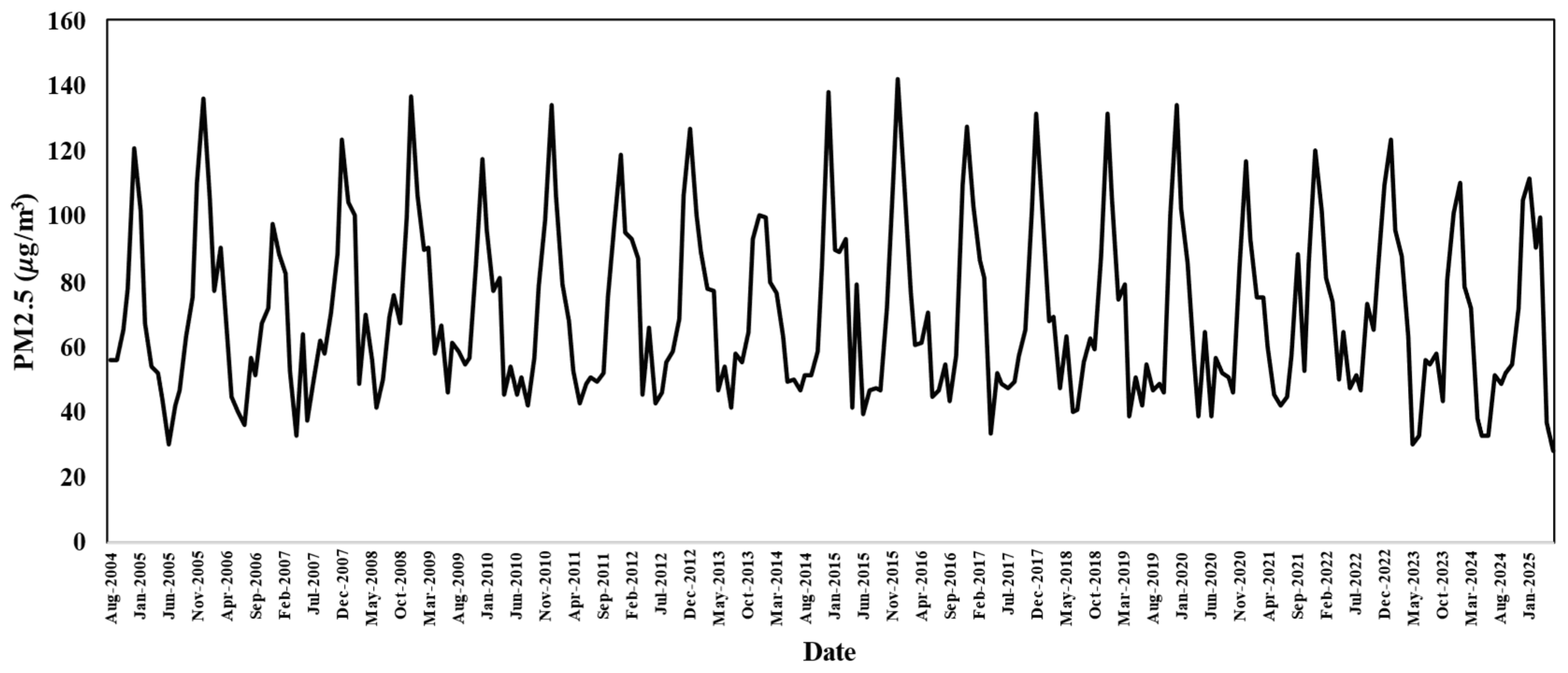
The time series plot (Figure 2) exhibits a clear seasonal pattern without any discernible long-term trend, indicating stationarity in both mean and variance. This observation was formally confirmed by the Augmented Dickey–Fuller (ADF) test, which yielded a Dickey–Fuller statistic of −12.101 with a p-value of 0.01 at lag order 6. Since the p-value is less than 0.05, the null hypothesis of a unit root was rejected, confirming that the time series is stationary and does not require differencing or further transformation before modeling.

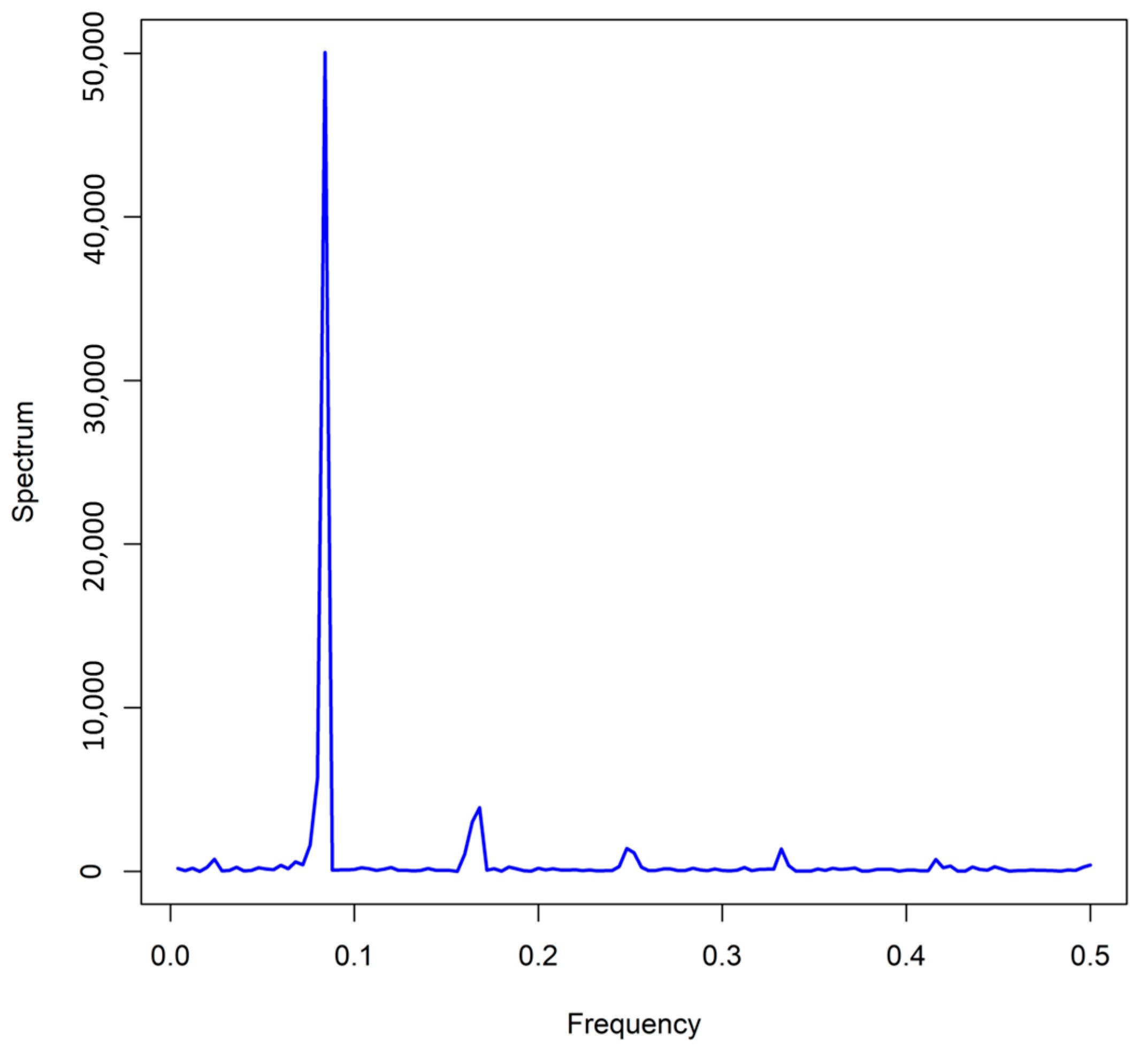
Figure 3 displays the periodogram of monthly PM_2.5 concentrations at Zabol station. The results reveal a dominant peak at a frequency of 0.083, corresponding to 12 months, indicating a strong annual seasonal pattern in the data. This finding aligns with previous observations of seasonal air pollution variations in the region. The absence of other significant peaks in the periodogram suggests no secondary cycles (such as semi-annual or short-term seasonal patterns) are present in the data. These results confirm the necessity of incorporating seasonal components, such as Fourier terms or SARIMA models, in subsequent analyses.

Figure 4 displays the Autocorrelation Function (ACF) and Partial Autocorrelation Function (PACF) plots of the PM_2.5 time series. The ACF plot clearly shows significant spikes at lag 12 and its multiples (24, 36, …), indicating a strong seasonal pattern with a 12-month periodicity. This pattern confirms that PM_2.5 concentrations are influenced by seasonal factors (such as climatic variations or periodic human activities). In contrast, the ACF fluctuations at non-seasonal lags (1 to 11) decay rapidly, suggesting the absence of long-term dependencies or trends in the data. The PACF plot reveals a significant spike at lag 12, which shows a notable decrease by lag 24. This behavior suggests that the seasonal component likely has a low order. Additionally, the slight increase at lag 1 in the PACF may indicate a non-seasonal autoregressive (AR) component. Based on the ACF and PACF analysis, we propose a SARIMA model structure to capture both the seasonal and non-seasonal components of the PM_2.5 time series. For the non-seasonal component (p,d,q), the rapid decay in the ACF and the significant spike at lag 1 in the PACF suggest either an AR(1) or MA(1) process, leading to our recommendation of p = 1 (non-seasonal AR term) and q = 1 (non-seasonal MA term). Regarding the seasonal component (P,D,Q) [12], the significant spike at lag 12 in the ACF with gradual decay indicates a seasonal AR(1) (P = 1) process, while the PACF’s spike at lag 12 without subsequent spikes suggests a seasonal MA(1) (Q = 1) component. Consequently, our final model proposal is SARIMA (1,0,2) (2,0,2) [12], which effectively accounts for both the observed short-term dependencies through its non-seasonal terms and the strong annual seasonality through its seasonal components. This model structure is particularly suitable given the clear 12-month periodicity evident in both plots and the relatively simple non-seasonal pattern. The inclusion of first-order seasonal AR and MA terms (P = 1, Q = 1) appropriately captures the persistent seasonal effects while maintaining model parsimony.

4.2. Model Estimation and Parameter Results

The estimated coefficients and standard errors for each fitted model are reported in

Table 1. Estimated parameters for SARIMA (1,0,2) (2,0,2) [12].

Coefficient	AR1	MA1	MA2	SAR1	SAR2	SMA1	SMA2	Mean
Estimates	−0.861	1.045	0.127	1.175	−0.183	−0.978	0.220	68.21
S.E.	0.124	0.136	0.072	0.504	0.501	0.493	0.384	7.073

,

Table 2. Estimated parameters for SARIMAX (0,0,0) (2,0,0) [12] with two Fourier pairs.

Coefficient	SAR1	SAR2	Intercept	S1-12	C1-12	S2-12	C2-12	${\mathit{\delta }}_1$	${\mathit{\delta }}_2$
Estimates	0.144	0.154	69.57	6.44	−26.16	−4.51	6.37	26.69	−18.61
S.E.	0.065	0.066	0.881	1.23	1.25	1.24	1.22	3.58	3.11

and

Table 3. Estimated parameters for TBATS.

Coefficient	$\mathit{\beta }$	${\mathit{\gamma }}_1$	${\mathit{\gamma }}_2$
Estimates	0.131	0.325	0.347
S.E.	0.062	0.059	0.061

. For the SARIMA (1,0,2) (2,0,2) [12] model (Table 1), the estimated autoregressive and moving average terms were statistically significant, indicating strong persistence and seasonal dependence in the PM_2.5 series. The model provided a parsimonious yet robust representation of both short-term and annual cycles.

The estimated parameters for the SARIMA (1,0,2) (2,0,2) [12] model reveal a complex and persistent structure in the PM_2.5 time series. The significant negative AR(1) coefficient (−0.861) indicates a strong mean-reverting pattern, where an increase in concentration in one month is typically followed by a decrease in the next. The significant MA terms further capture these short-term dynamics; the strong positive MA(1) coefficient (1.045) suggests that random shocks, such as sudden dust storms, have an immediate and pronounced impact on PM_2.5 levels, while the weaker MA(2) term shows this influence weakly persists for a second month. The model’s seasonal components are particularly dominant. The powerful and significant SAR(1) coefficient (1.175) confirms a robust annual cycle, demonstrating that concentrations in a given month are heavily dependent on those from the same month in the previous year. This is complemented by the significant negative SMA(1) coefficient (−0.978), which effectively models and dampens seasonal shocks. Finally, the estimated mean value of 68.21 μg/m³ signifies a chronically high background level of air pollution, far exceeding WHO guidelines. Collectively, these parameters affirm the model’s ability to parsimoniously yet robustly represent both the short-term autoregressive moving-average dynamics and the dominant seasonal forces governing dust concentrations in Zabol.

Table 2 shows the results of the SARIMAX (0,0,0) (2,0,0) [12] model with two Fourier pairs and confirms that the seasonality is overwhelmingly deterministic. This is evidenced by the highly significant and large-magnitude Fourier coefficients (e.g., −26.16 and 6.44 for the first harmonic), which dominate the model, in stark contrast to the weak and modest seasonal autoregressive parameters (0.144 and 0.154). The analysis confirms that employing Fourier terms is the primary driver for capturing the dominant 12-month periodicity and achieving predictive accuracy, while the included exogenous variables also demonstrate a strong and significant influence with their substantial coefficients (26.69 and −18.61).

Finally, the TBATS model (Table 3) captured complex seasonal components through its trigonometric and trend-related terms, all of which were significant. This highlights TBATS as a flexible alternative for representing overlapping or evolving seasonalities.

Collectively, the results indicate that SARIMA offers a simple and statistically adequate structure, SARIMAX leverages deterministic cycles via Fourier components, and TBATS provides enhanced flexibility for more complex seasonal dynamics.

Table 4. Estimated parameters for the Hybrid model.

Coefficient	${\mathit{\omega }}_1$	${\mathit{\omega }}_2$	${\mathit{\omega }}_3$
Estimates	0.109	0.628	0.263
S.E.	0.031	0.044	0.041

presents the weight estimates for the hybrid ensemble model, which combines forecasts from SARIMA, SARIMAX, and TBATS models. The weights were optimized by minimizing the Root Mean Square Error (RMSE), resulting in a configuration where SARIMAX receives the highest weight (ω₂ = 0.628), followed by TBATS (ω₃ = 0.263), and SARIMA (ω₁ = 0.109). The significant magnitude of the SARIMAX weight underscores its dominant role, consistent with earlier findings that highlighted its effectiveness in modeling deterministic seasonality and incorporating exogenous variables. Meanwhile, the substantial weight assigned to TBATS suggests it captures complex seasonal patterns or nonlinearities not fully addressed by the other models. All weights are statistically significant, as each estimate is multiple times larger than its standard error, confirming their robustness.

The hybrid approach successfully leverages the distinct strengths of each model: SARIMAX provides a strong baseline with its ability to handle external regressors and deterministic seasonality, TBATS adds flexibility for intricate seasonal behaviors, and SARIMA contributes a parsimonious seasonal ARIMA structure. By integrating these components, the ensemble mitigates individual model biases and variances, resulting in improved forecast accuracy and robustness. This strategy demonstrates the value of model combination in enhancing predictive performance beyond what any single model can achieve.

4.3. Model Validation and Diagnostic Checks

Table 5. Model comparison using statistical criteria (AIC, BIC, RMSE, MAE, MAPE).

Criteria	AIC	BIC	RMSE (μg/m3)	MAE (μg/m3)	MAPE
SARIMA	1946.27	1977.96	10.852	8.590	13.860
SARIMAX	1866.45	1901.67	9.69	7.52	11.64
TBATS	2574.202	2623.502	10.295	8.123	13.601
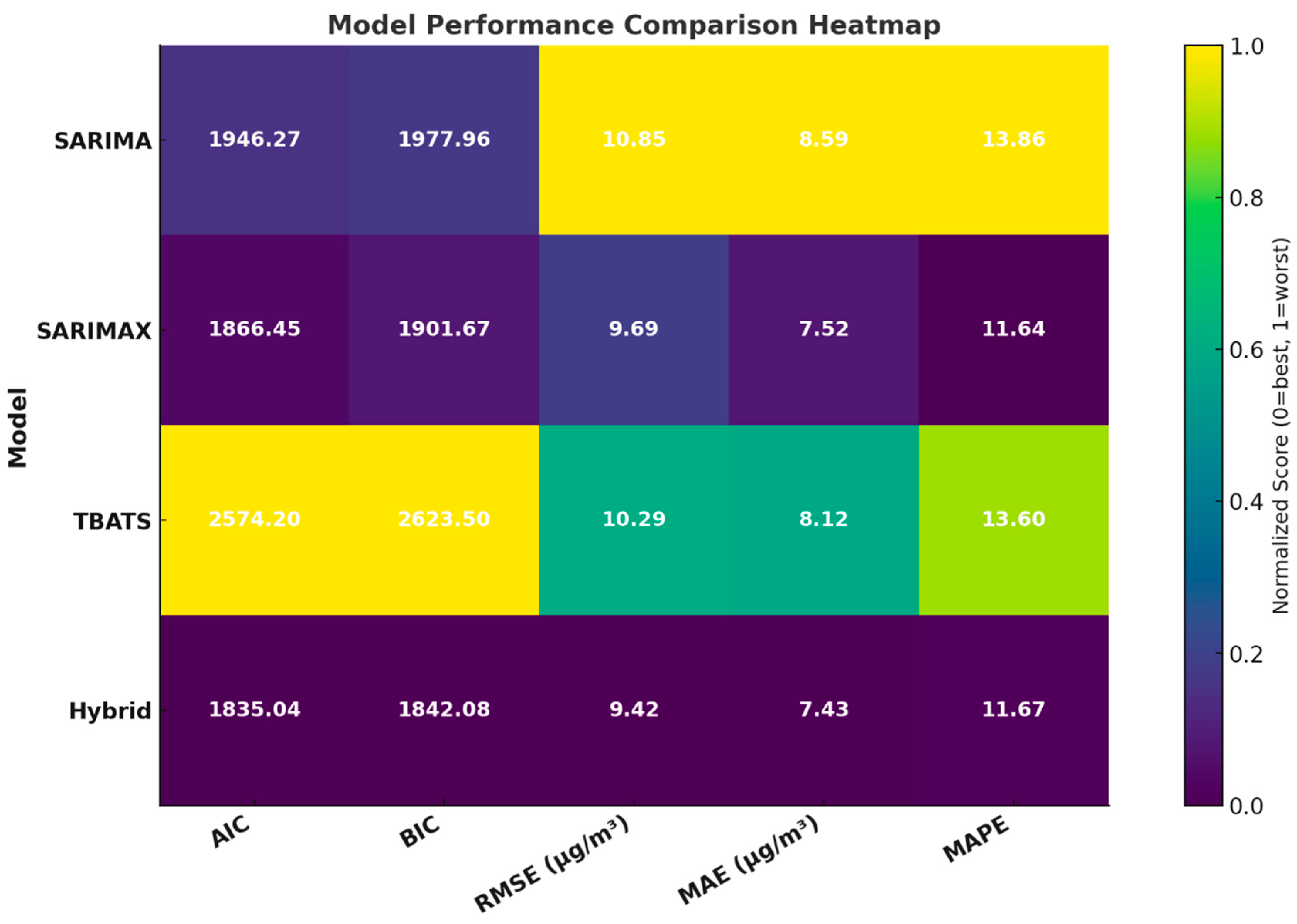
Hybrid	1835.04	1842.08	9.42	7.43	11.67

and Figure 5 present a comprehensive performance evaluation of four forecasting models: SARIMA, SARIMAX, TBATS, and a Hybrid ensemble. The results clearly demonstrate that the Hybrid model achieves the best overall performance, with the lowest AIC (1835.04) and BIC (1842.08) values, indicating superior goodness-of-fit while maintaining optimal parsimony. Furthermore, it delivers the smallest RMSE (9.42) and MAE (7.43), highlighting its exceptional predictive accuracy and ability to minimize absolute errors. While its MAPE (11.67%) is slightly higher than that of the SARIMAX model, this marginal difference is outweighed by its advantages in other critical metrics.

The SARIMAX model remains the strongest individual model, outperforming both the standalone SARIMA and TBATS models across all criteria, including AIC (1866.45), BIC (1901.67), RMSE (9.69), MAE (7.52), and MAPE (11.64%). This confirms its robustness in leveraging exogenous variables and capturing key data patterns. In contrast, the TBATS model shows the weakest statistical fit with the highest AIC and BIC values, though it performs reasonably in point forecasting accuracy. The SARIMA model serves as a decent baseline but is consistently outperformed by its more sophisticated counterparts. Ultimately, the analysis confirms that the Hybrid model’s strategy of combining individual forecasts yields the most robust and accurate predictions, making it the recommended choice for this forecasting task.

Table 6. Ljung–Box test results for model residuals.

Model/Statistics	Q*	df	p-Value
SARIMA	18.556	17	0.354
SARIMAX	13.071	22	0.93
TBATS	37.397	24	0.039
Hybrid	15.311	21	0.882

presents the Ljung–Box test results for residual autocorrelation across the four models, providing crucial insights into their statistical adequacy. The Hybrid model demonstrates the best performance with a test statistic of Q* = 15.311 and a high p-value of 0.882, indicating no significant residual autocorrelation and confirming its ability to effectively capture temporal dependencies through its ensemble approach. Similarly, the SARIMAX model shows excellent results (Q* = 13.071, p = 0.93), validating its strong capacity to model patterns using exogenous variables. The SARIMA model also performs acceptably (Q* = 18.556, p = 0.354), showing no concerning autocorrelation in its residuals. In stark contrast, the TBATS model exhibits significant residual autocorrelation (Q* = 37.397, p = 0.039), revealing substantial limitations in accounting for all temporal patterns. These diagnostic results complement the earlier performance metrics, confirming that both the Hybrid and SARIMAX models not only excel in predictive accuracy but also provide the most statistically adequate residual structures, with the Hybrid model emerging as the most comprehensive solution.

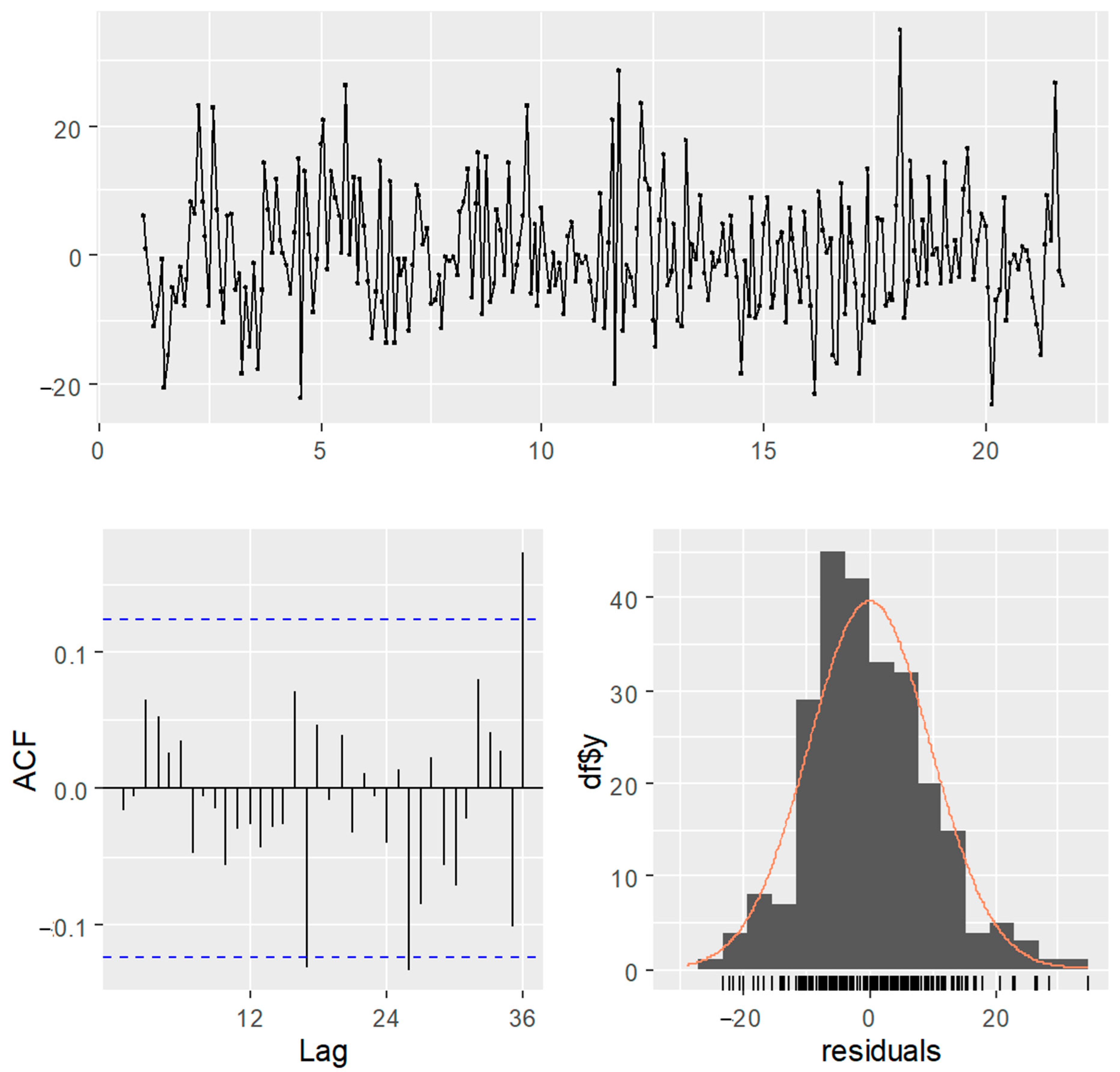
Figure 6 displays the residual diagnostics for the SARIMAX (0,0,0) (2,0,0) [12] model, which includes three key components: the residual time series plot (top), the autocorrelation function (ACF) of residuals (bottom left), and a histogram of residuals with a density overlay (bottom right). The residual time series plot shows that the residuals fluctuate randomly around zero without any discernible systematic patterns or trends, indicating that the model has effectively captured the underlying structure of the data. The ACF plot reveals no significant autocorrelations at any lag, as all bars remain within the confidence bounds, suggesting that the model has adequately accounted for temporal dependencies, including seasonal effects. Additionally, the histogram of residuals exhibits a roughly symmetric distribution that aligns well with the normal density curve, supporting the assumption of normality. Collectively, these diagnostics confirm that the SARIMAX (0,0,0) (2,0,0) [12] model is well-specified, with residuals behaving as white noise. For further validation, statistical tests such as the Ljung–Box test (for autocorrelation) or the Shapiro–Wilk test (for normality) could be conducted, but the visual evidence strongly suggests the model’s adequacy for forecasting purposes.

Collectively, these results indicate that the SARIMAX model with Fourier terms provides the most robust fit for the monthly PM_2.5 series in Zabol, outperforming both the classical SARIMA and TBATS models in terms of statistical fit and residual diagnostics.

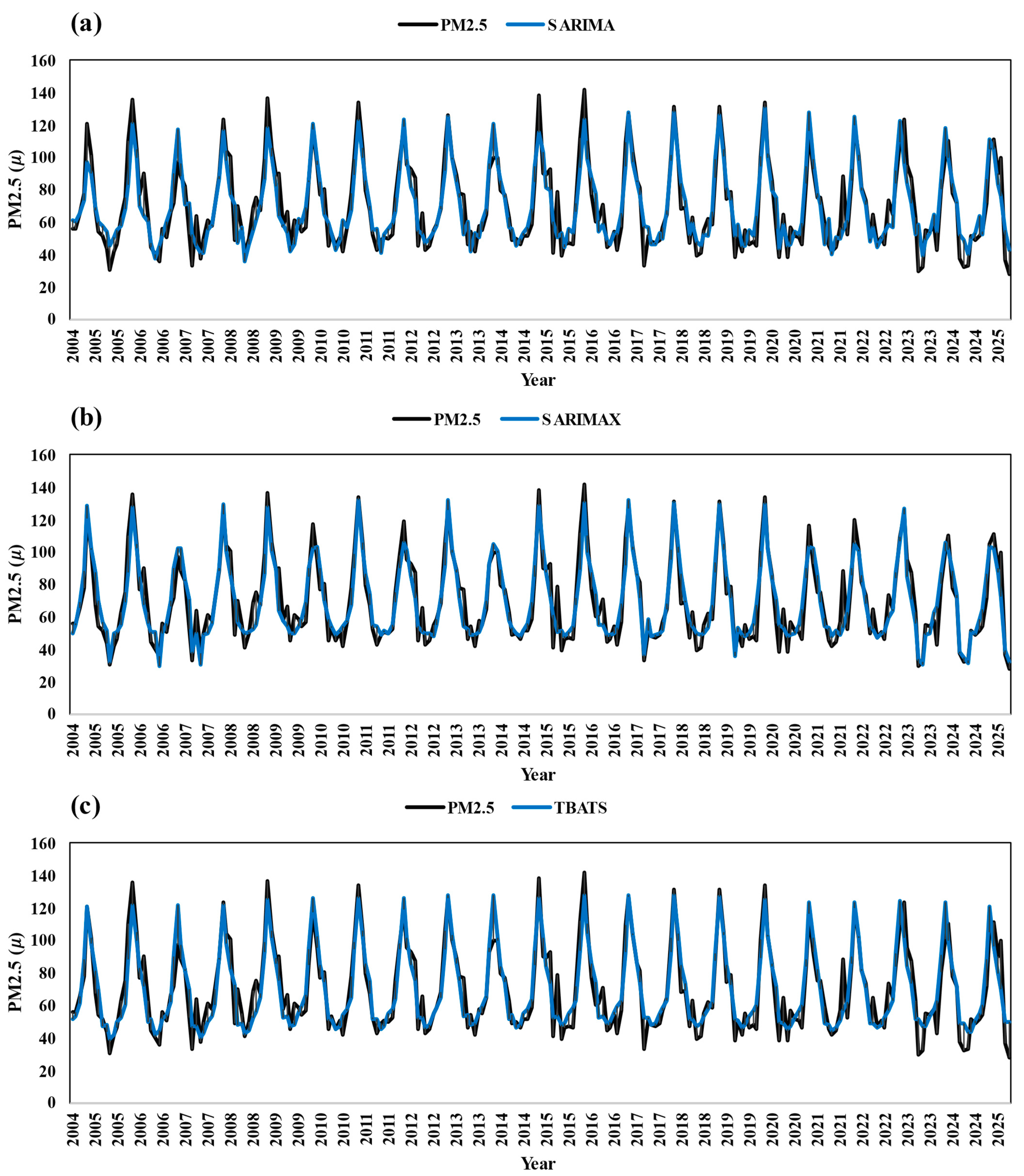
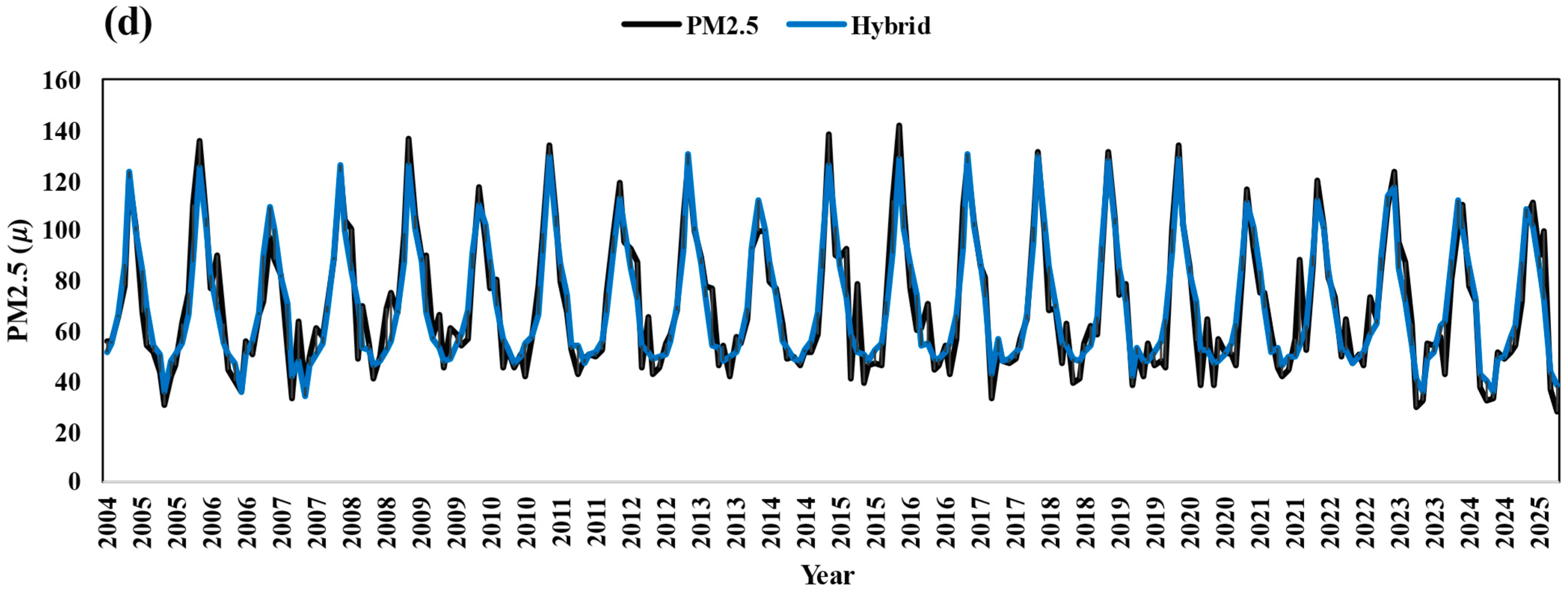
As shown in Figure 7a–d, the comparison between observed and forecasted PM_2.5 concentrations at Zabol station from 2004 to 2025 is presented using different models.

4.4. Out-of-Sample Forecasting with the Hybrid Model

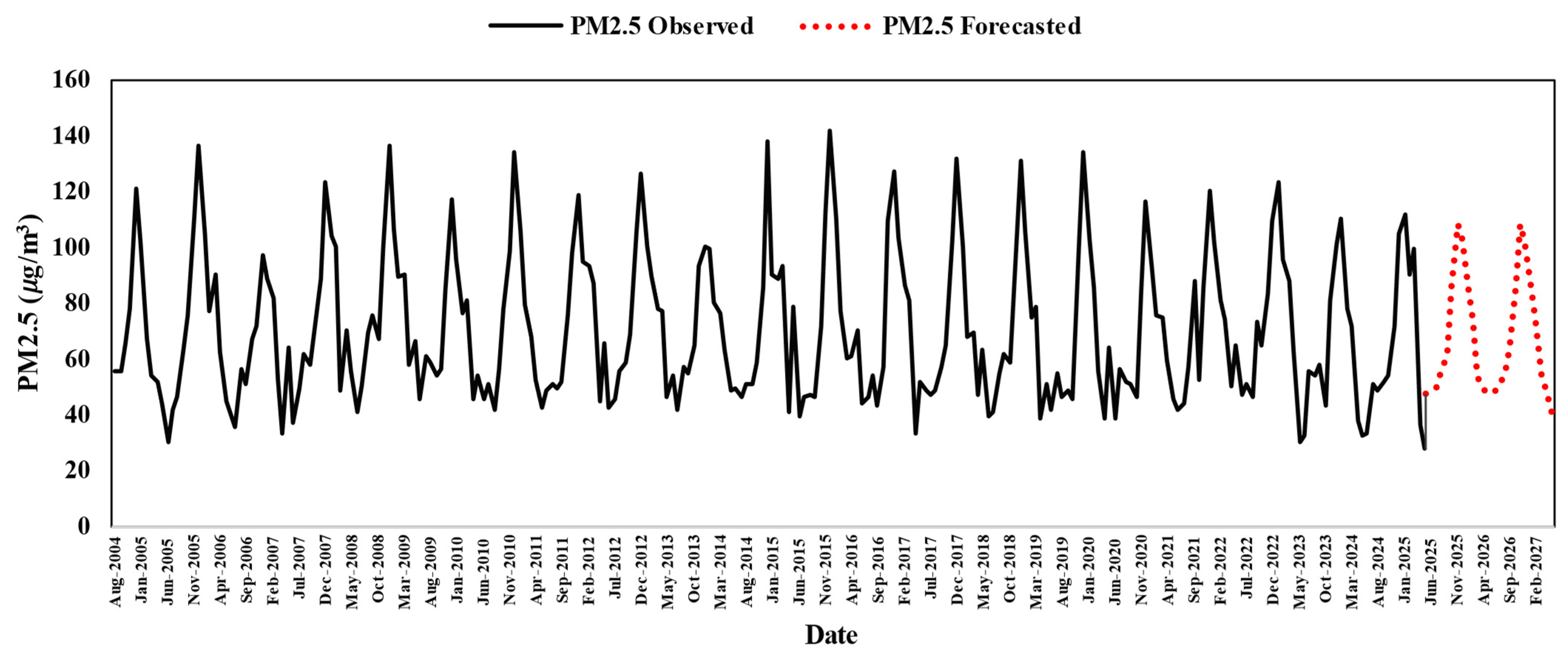
Figure 8 displays the observed and forecasted monthly PM_2.5 concentrations in Zabol from 2004 to 2027, generated by the Hybrid model. As clearly shown, the model has successfully captured the seasonal pattern of the historical data. Both the short-term and long-term forecasts (up to 2027) follow the anticipated trends with reasonable accuracy, and the forecasted peak values for the upcoming periods (such as 2026–2027) appear to be more conservative and lower compared to the past observed peaks (like in 2014–2015). Overall, the model demonstrates stable and reliable performance not only for short-term forecasting and seasonal planning but also for the long-term outlook up to 2027. The figure effectively demonstrates the model’s strength in capturing and continuing the seasonal variation pattern.

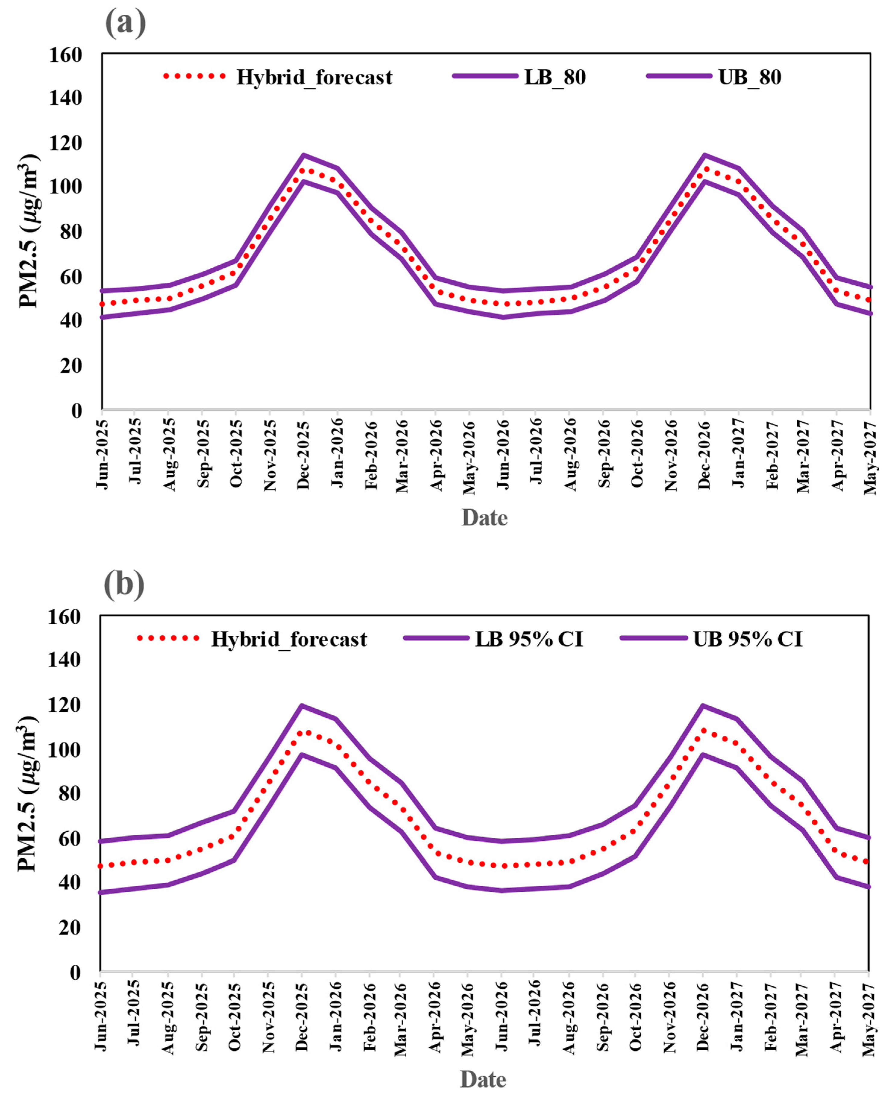
Figure 9a displays the PM_2.5 concentration forecasts generated by the hybrid model with an 80% confidence interval. The red line represents the mean predicted values for each month, while the blue shaded band around this line indicates the 80% confidence interval range defined by the lower bound (LB_80) and upper bound (UB_80).

Contrary to typical forecasting models, the width or difference between these bounds remains constant throughout the entire forecast period from June 2025 to May 2027. Calculations based on the data show that the difference between the upper and lower bounds is precisely 11.386 μg/m³ for all months. For example, in June 2025, the forecast range is from 41.55 to 52.93 μg/m³, in December 2026 from 102.62 to 114.01 μg/m³, and in May 2027 from 43.49 to 54.88 μg/m³. This complete stability in the confidence band width, despite significant variations in the central predicted values ranging from approximately 47 to 108 μg/m³, indicates that the hybrid model has considered a constant absolute uncertainty for the entire two-year forecast horizon. Therefore, unlike many forecasting models where uncertainty increases with longer time horizons, this model demonstrates the same level of accuracy and uncertainty throughout the entire forecast period.

Figure 9b displays the 95% confidence interval forecasts generated by the hybrid model.

Contrary to initial expectations, the width of this confidence interval remains constant throughout the entire forecast period from June 2025 to May 2027. The difference between the upper and lower bounds is consistently 22.252 μg/m³ across all months, with no observable expansion in the interval width over time. For example, in June 2025, the forecast range spans from 36.11 to 58.37 μg/m³, in December 2026 from 97.18 to 119.43 μg/m³, and in May 2027 from 38.06 to 60.31 μg/m³. This consistent interval width, despite significant fluctuations in the central predicted values, indicates that the model maintains a stable level of uncertainty throughout the entire two-year forecast horizon. The 95% confidence interval provides a wider range of potential outcomes compared to the 80% interval, but unlike typical forecasting models, this range does not expand with longer prediction horizons. Therefore, both confidence levels demonstrate consistent performance across short-term and long-term forecasts, suggesting the model’s reliability remains constant throughout the prediction period.

Overall, the Hybrid model demonstrates reliable predictive performance for seasonal dust episodes in Zabol, as evidenced by the close alignment between forecasted values and historical observations, along with reasonably tight confidence bounds. This underscores the suitability of the Hybrid modeling approach for operational air quality management and public health planning in regions characterized by pronounced seasonal variability in PM_2.5 levels.

5. Discussion

The present study aims to predict PM_2.5 concentrations at the Zabol station using SARIMA, SARIMAX, TBATS, and a Hybrid model on a monthly scale from 2004 to 2025. The selection of these classical models, along with the Hybrid ensemble approach, over more complex machine learning-based methods such as LSTM or XGBoost, is primarily due to the limitations of observational data in this region and the need for models with higher interpretability and manageable parameter complexity [55]. Classical time series models, particularly in cases where data exhibit clear seasonal patterns—such as PM_2.5 in Zabol—demonstrate acceptable performance even with limited data volume. The Hybrid model further enhances predictive robustness by combining the strengths of individual models.

Preliminary data analysis revealed a strong seasonal pattern without a long-term trend, which was confirmed by the ADF test. The periodogram also identified an annual cycle with a frequency of 0.083 (a 12-month period), reinforcing the necessity of incorporating seasonal components in the modeling. ACF/PACF analysis further emphasized that seasonal dependencies at lags 12, 24, etc., are dominant.

According to the findings of Rashki et al. [56,57] and Behrooz et al. [15], the seasonal pattern of PM_2.5 concentration in Zabol is primarily influenced by the 120-day winds of Sistan, with the highest levels of these particles observed during summer (June to September). This significant increase in particle concentration stems from the key role of these strong winds in transporting dust from adjacent arid regions, particularly the deserts of Afghanistan and the Sistan Plain, to the Zabol area. This process not only leads to worsening air pollution but also significantly impacts air quality degradation and increases health risks for residents during this period. Such findings highlight the necessity of considering regional climatic factors and wind patterns in air pollution management and environmental planning. Furthermore, recurrent droughts and the desiccation of Hamoun Wetland (resulting from reduced water inflow from the Hirmand River) during spring and summer exacerbate local dust emissions by decreasing soil moisture [58].

Although statistical time-series models do not explicitly account for causal drivers such as emission sources or meteorological dynamics, they remain widely adopted and validated for short- to medium-term air quality forecasting [8,19,59]. In highly seasonal environments like Zabol, where the “120-day wind” imposes a strong deterministic cycle, the Hybrid model—integrating SARIMA, SARIMAX, and TBATS—proves capable of reproducing recurrent dust episodes with improved accuracy. As such, the forecasts generated here should not be interpreted as substitutes for process-based or emission-driven models, but rather as complementary tools that provide operational value for early-warning and public health protection in data-scarce regions.

The evaluation of model accuracy and goodness-of-fit indicated that the Hybrid model, with its weighted combination of SARIMA, SARIMAX, and TBATS, outperformed all individual models. It achieved the lowest AIC (1835.04) and BIC (1842.08), along with the smallest RMSE (9.42) and MAE (7.43), demonstrating its superior predictive accuracy and robustness. The Ljung–Box test further confirmed the Hybrid model’s dominance in residual diagnostics (Q = 15.311, p = 0.882), unequivocally verifying its capacity to eliminate temporal dependencies. In contrast, SARIMAX showed strong performance but with minor residual autocorrelation (p = 0.93), while TBATS exhibited significant limitations (p = 0.039). This empirical evidence corroborates established theoretical frameworks [14,22] that advocate for model parsimony and ensemble techniques when confronting linearly structured environmental time series.

This superiority aligns with broader findings in the field. In this context, Chai et al. [60] demonstrated that integrating satellite-based predictors with machine learning models substantially improves PM_2.5 estimation accuracy in China, further supporting the broader potential of hybrid frameworks for air quality applications. Our results reinforce this paradigm, showing that even without satellite data, a hybrid approach combining classical time-series models can significantly enhance prediction robustness in data-scarce regions.

The TBATS model exhibited significant residual autocorrelation (Ljung–Box p = 0.039), indicating its inability to fully capture the data’s temporal dependencies. This limitation may arise from the model’s reliance on trigonometric seasonality, which struggles to adapt to the rigid, meteorologically driven annual cycle dominated by the 120-day Sistan winds. Additionally, TBATS may not adequately account for abrupt dust events causing short-term shocks. Alternative configurations (e.g., increasing harmonics or enabling ARMA errors) were tested but did not yield improved results, suggesting inherent incompatibility with this dataset’s structure [51].

Out-of-sample forecast analysis using the Hybrid model demonstrates its effectiveness in capturing the seasonal patterns of PM_2.5 concentrations in Zabol [58]. Contrary to conventional expectations, as the forecast horizon extends to 2026–2027, the model’s uncertainty does not progressively increase but rather maintains constant levels of uncertainty throughout the entire forecast period. The Hybrid model demonstrates constant absolute uncertainty over the two-year forecast horizon, with the 80% confidence interval consistently maintaining a fixed width of 11.386 μg/m³ and the 95% confidence interval maintaining a constant width of 22.252 μg/m³. This consistent pattern persists even when PM_2.5 concentrations exceed the 100 μg/m³ threshold, indicating the model’s ability to maintain the same level of accuracy for extreme values. Although the Hybrid model has successfully maintained consistent uncertainty levels, it is worth noting that this characteristic may stem from inherent limitations in accounting for cumulative error propagation in multi-step predictions and structural deviations caused by long-term climatic variations [59,61,62]. This finding suggests that while the model demonstrates consistent performance for both short-term and long-term predictions, it may face challenges in fully capturing the inherent uncertainty in long-term forecasts.

Unlike many conventional time series models, the hybrid model developed in this study does not exhibit cumulative error dependency in multi-step-ahead predictions. As observed in the results, the confidence interval bandwidth remains completely stable throughout the entire forecast period from June 2025 to May 2027. This stability indicates that the model possesses high resistance to error propagation and accumulation, maintaining the same level of accuracy even over long-term forecast horizons [63,64].

Beyond the specific case of Zabol, the proposed Hybrid framework has potential for broader applications. Similar arid and dust-prone regions such as the Middle East, Central Asia, and North Africa face persistent dust episodes driven by deterministic seasonal cycles but often lack dense monitoring networks. In such settings, integrating spectral diagnostics with classical time-series forecasting and ensemble techniques can provide a cost-effective and interpretable early-warning tool. Moreover, this methodological structure can be extended to other environmental variables with strong cyclic behavior, such as ozone concentrations, temperature anomalies, and rainfall extremes, thereby enhancing its transferability and practical relevance [65,66].

6. Conclusions

This study developed and evaluated a suite of time series models, including SARIMA, SARIMAX, TBATS, and a novel Hybrid ensemble, for forecasting monthly PM_2.5 concentrations in Zabol, Iran, using data from 2004 to 2025. The key finding was that the Hybrid model, which intelligently combines the forecasts of the three individual models through an optimized weighting scheme, demonstrated superior performance across all evaluation metrics, achieving the lowest AIC, BIC, RMSE, and MAE. This result underscores the significant advantage of leveraging ensemble techniques to integrate the strengths of diverse modeling approaches.

The research revealed several critical insights about dust forecasting in arid regions. First, it demonstrates that a hybrid approach, rather than relying on a single complex model, can most effectively capture the physical processes governing dust transport, as evidenced by the Hybrid model’s optimal weights. Second, the study highlights how regional climatic factors—particularly the Sistan wind regime and Hamoun wetland desiccation—create a strong, deterministic seasonal pattern that was best captured by the Fourier terms in the SARIMAX model.

Several limitations warrant consideration. Dependence on limited observational data presents additional challenges. These limitations suggest that while the Hybrid model provides a solid foundation, it could be further enhanced by complementing it with other approaches for comprehensive dust forecasting. Additionally, the absence of meteorological variables such as relative humidity, temperature anomalies, and wind speed fluctuations represents a further limitation. The inclusion of these factors through reanalysis of datasets or remote sensing could enhance predictive performance.

Future research directions should focus on advancing hybrid modeling frameworks by integrating the interpretability of classical models with the pattern recognition capabilities of machine learning. Incorporating additional data sources like satellite observations and meteorological reanalysis could enhance prediction accuracy, particularly for extreme events. The development of more sophisticated ensemble forecasting systems would help quantify and communicate prediction uncertainty more effectively.

From a practical perspective, these findings support several policy recommendations. The demonstrated Hybrid forecasting approach could form the basis for early warning systems to protect public health during dust events. In particular, forecasts can be linked to health-relevant thresholds, where PM_2.5 levels above 35 µg/m³ correspond to the WHO 24 h guideline, and values exceeding 100 µg/m³—frequently observed during the 120-day wind season—represent a critical local risk threshold. Incorporating these benchmarks into operational use would enable timely alerts, targeted protective measures, and prioritization of vulnerable populations. The methodology therefore provides environmental managers with a powerful tool for anticipating air quality degradation and implementing mitigation strategies.

This research advances dust forecasting capabilities in several important ways. It provides a validated hybrid modeling framework adaptable to similar arid environments, offers new insights into the synergistic value of combining model types for seasonal forecasting, and establishes clear pathways for future improvements through integrated modeling approaches. The findings contribute to both the methodological development of environmental forecasting and the practical management of air quality in dust-affected regions.