
Wildfire Susceptibility Mapping in Greece Using Ensemble Machine Learning


Abstract
1. Introduction
2. Methods and Data
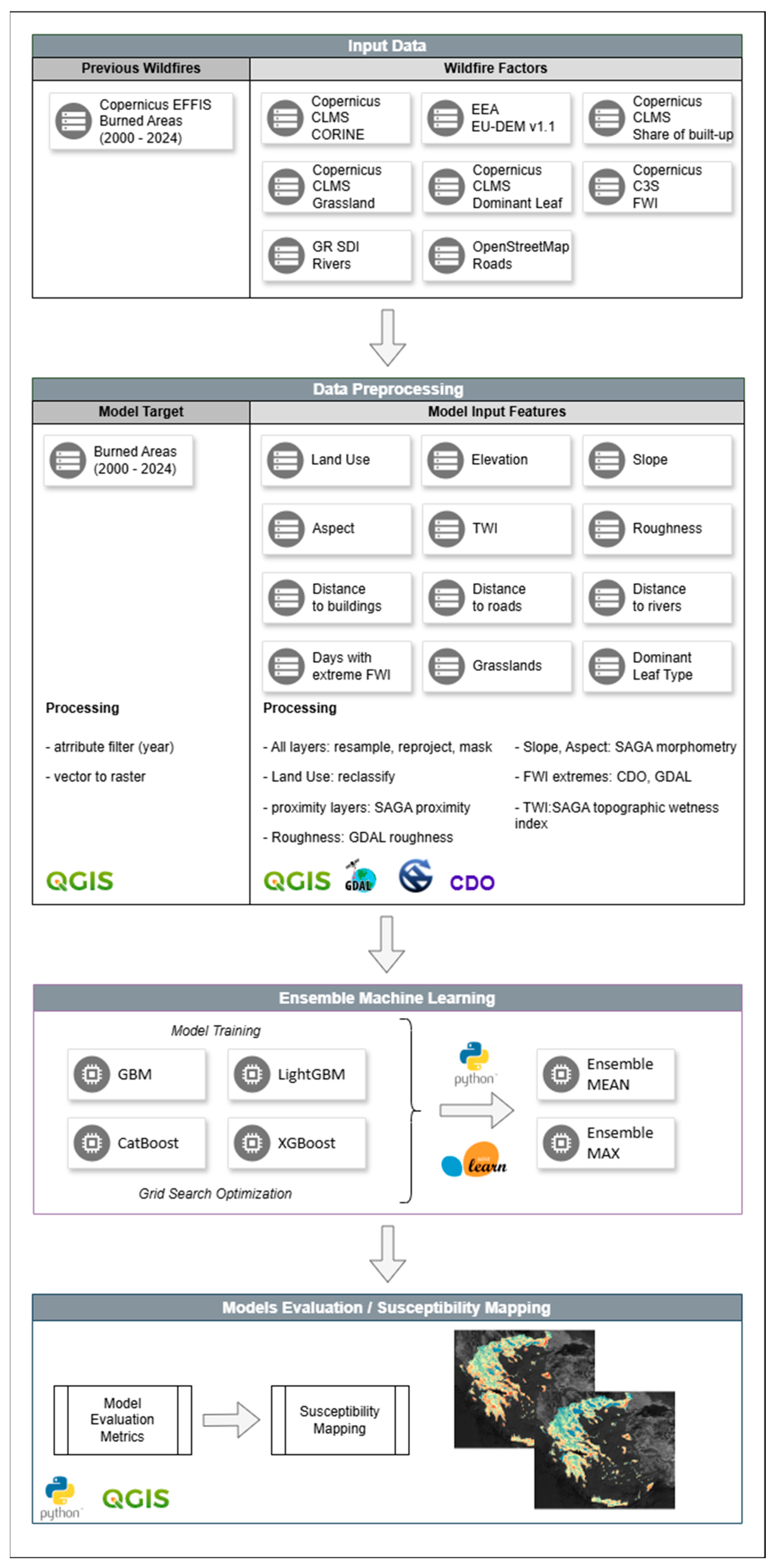
2.1. Methodology
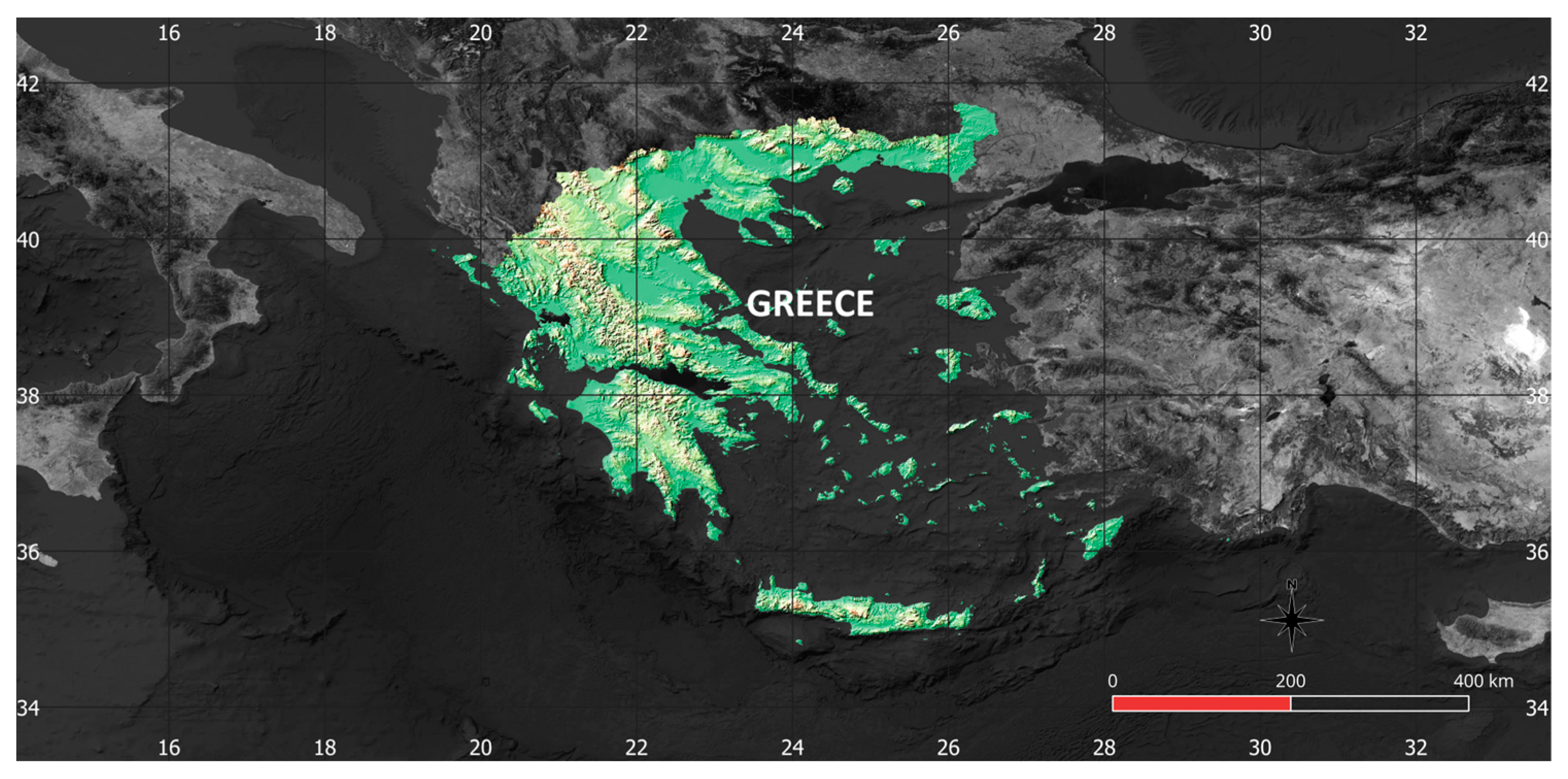
2.2. Study Area
2.3. Data
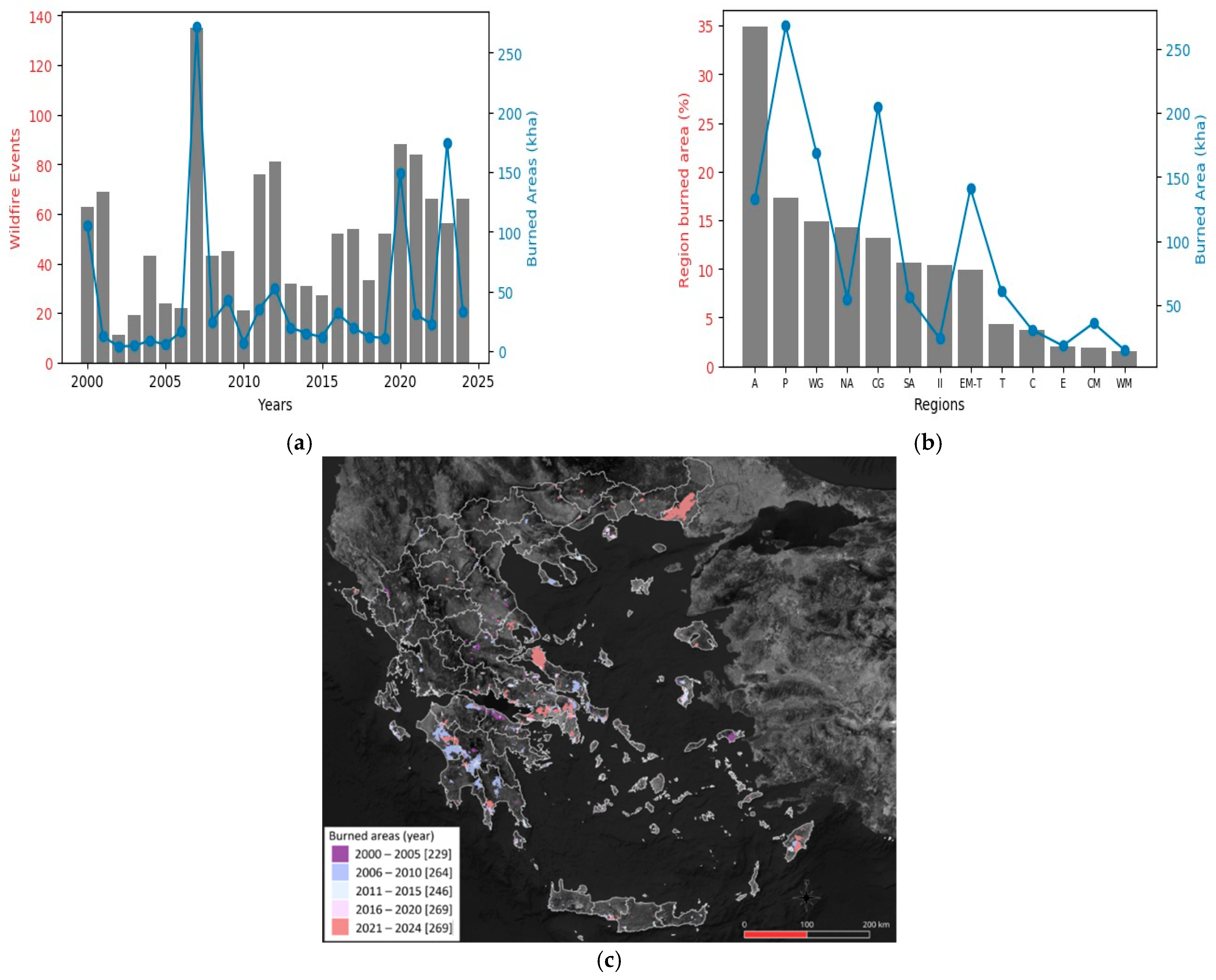
2.3.1. Previous Wildfires
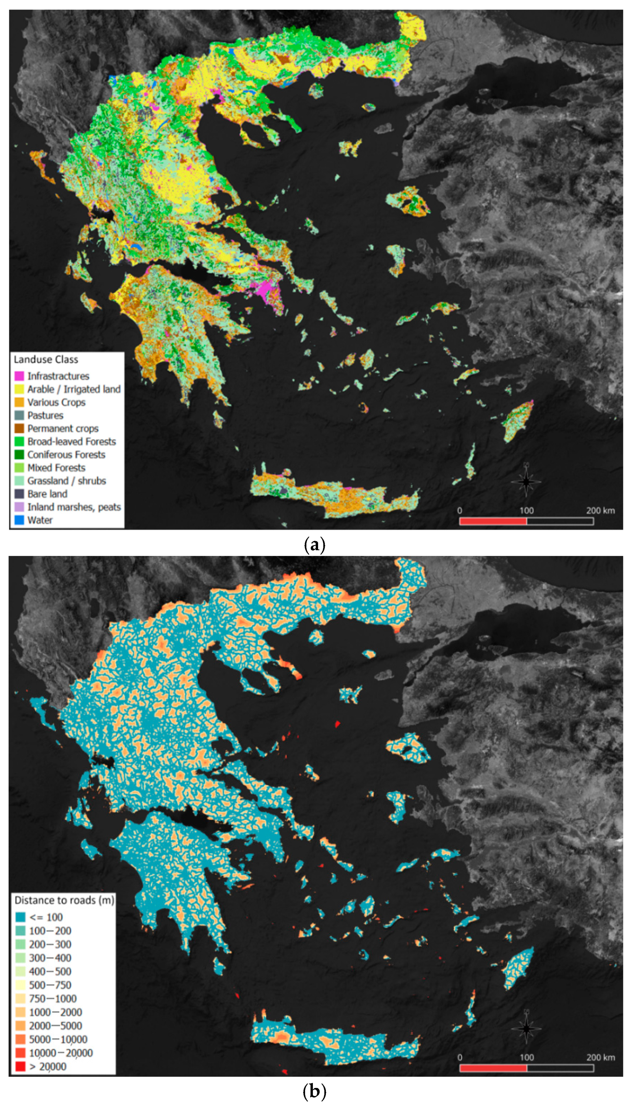
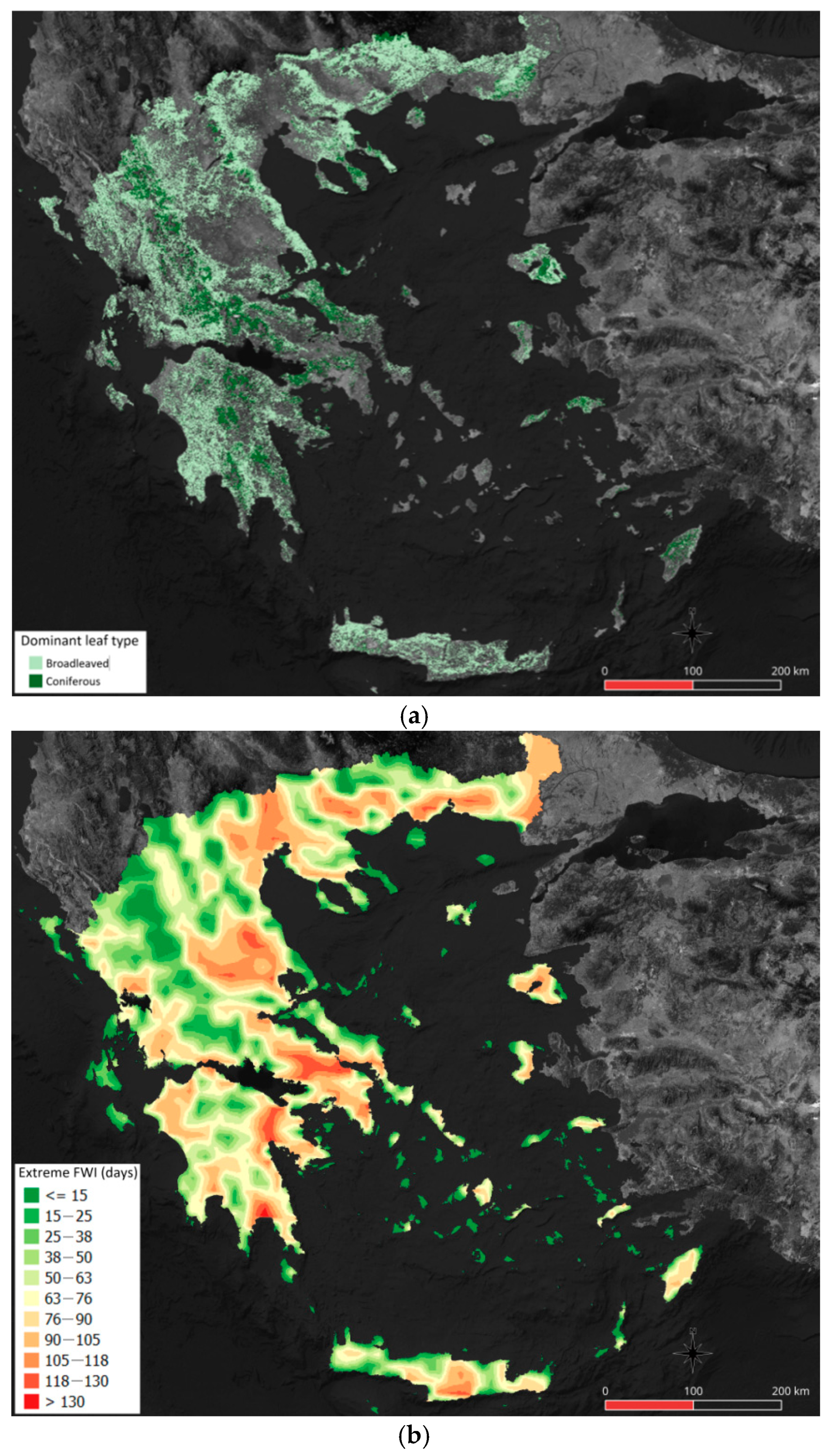
2.3.2. Wildfires Factors
3. Ensemble Methods
3.1. Extreme Gradient Boosting
3.2. Gradient Boosting Machine—Light Gradient Boosting Machine
3.3. Categorical Boosting
4. Simulation Setup and Results
4.1. Simulation Setup
4.1.1. Evaluation Metrics
4.1.2. XGBoost
4.1.3. GBM
4.1.4. LGBM
4.1.5. CatBoost
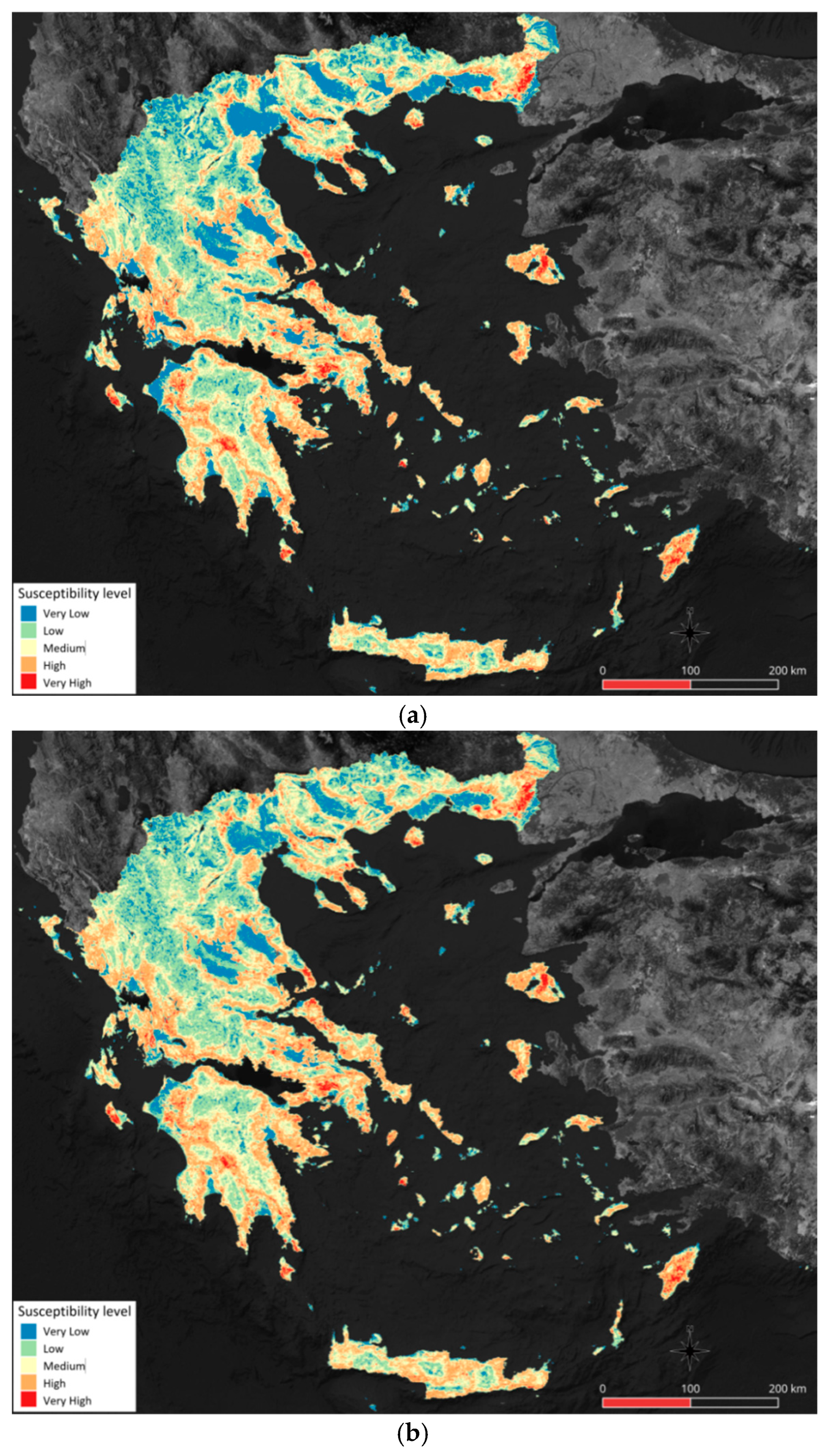
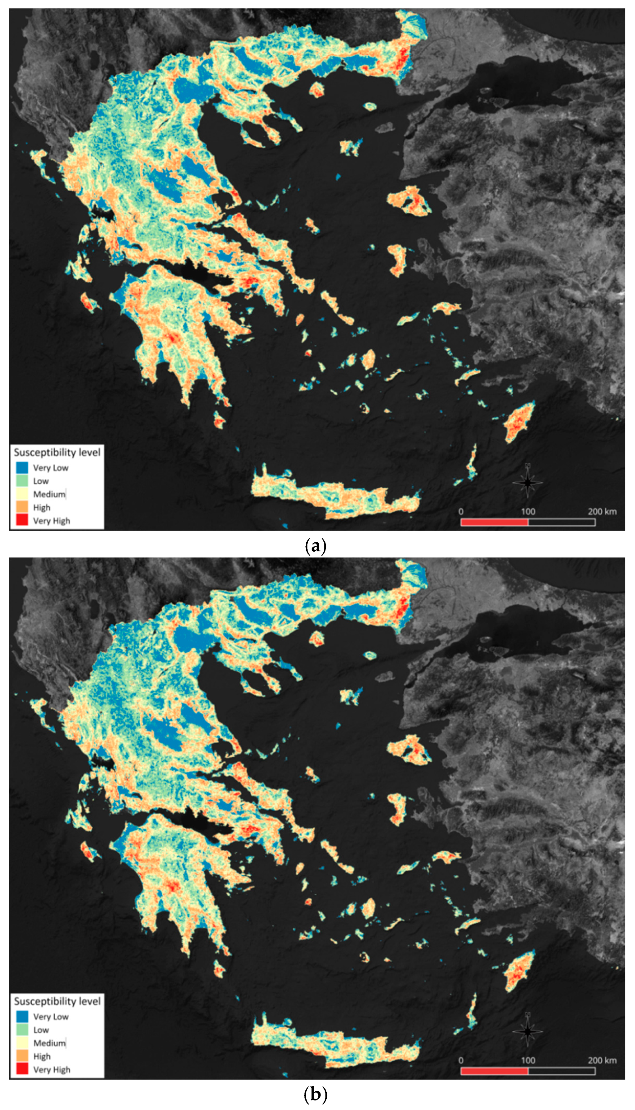
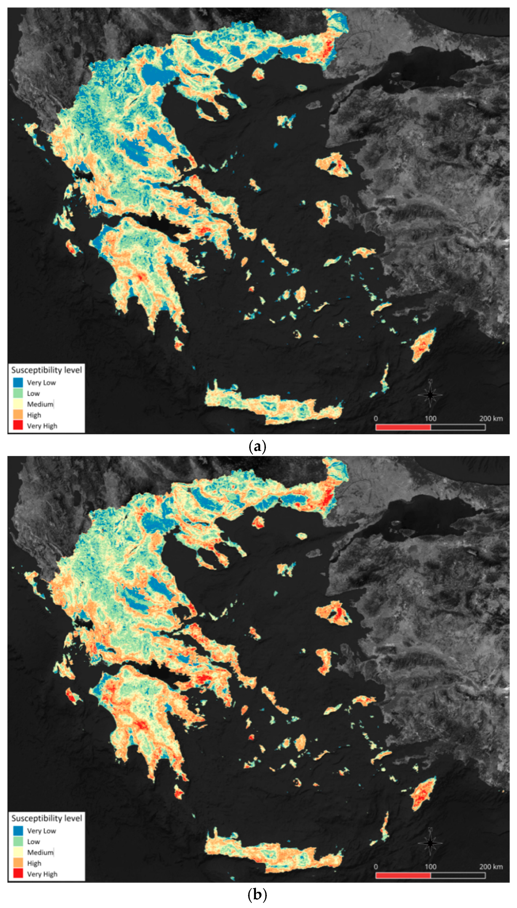
4.2. Simulation Results
5. Experimental Results
6. Conclusions
Author Contributions
Funding
Data Availability Statement
Conflicts of Interest
References
- Goleiji, E.; Hosseini, S.M.; Khorasani, N.; Monavari, S.M. Forest fire risk assessment—An integrated approach based on multicriteria evaluation. Environ. Monit. Assess. 2017, 189, 612. [Google Scholar] [CrossRef] [PubMed]
- Hwang, C.-L.; Yoon, K. Methods for Multiple Attribute Decision Making. In Multiple Attribute Decision Making; Lecture Notes in Economics and Mathematical Systems; Springer: Berlin/Heidelberg, Germany, 1981; Volume 186, pp. 58–191. [Google Scholar] [CrossRef]
- Ljubomir, G.; Pamučar, D.; Drobnjak, S.; Pourghasemi, H.R. Modeling the Spatial Variability of Forest Fire Susceptibility Using Geographical Information Systems and the Analytical Hierarchy Process. In Spatial Modeling in GIS and R for Earth and Environmental Sciences; Elsevier: Amsterdam, The Netherlands, 2019; pp. 337–369. [Google Scholar] [CrossRef]
- Samui, P. Support vector machine applied to settlement of shallow foundations on cohesionless soils. Comput. Geotech. 2008, 35, 419–427. [Google Scholar] [CrossRef]
- Oliveira, S.; Oehler, F.; San-Miguel-Ayanz, J.; Camia, A.; Pereira, J.M.C. Modeling Spatial Patterns of Fire Occurrence in Mediterranean Europe Using Multiple Regression and Random Forest. For. Ecol. Manag. 2012, 275, 117–129. [Google Scholar] [CrossRef]
- Michael, Y.; Helman, D.; Glickman, O.; Gabay, D.; Brenner, S.; Lensky, I.M. Forecasting fire risk with machine learning and dynamic information derived from satellite vegetation index time-series. Sci. Total Environ. 2021, 764, 142844. [Google Scholar] [CrossRef]
- Pourghasemi, H.R. GIS-based forest fire susceptibility mapping in Iran: A comparison between evidential belief function and binary logistic regression models. Scand. J. For. Res. 2016, 31, 80–98. [Google Scholar] [CrossRef]
- Dang, T.T.; Cheng, Y.; Mann, J.; Hawick, K.; Li, Q. Fire Risk Prediction Using Multi-Source Data: A case study in Humberside area. In Proceedings of the 2019 25th International Conference on Automation and Computing (ICAC), Lancaster, UK, 5–7 September 2019; IEEE: New York, NY, USA, 2019; pp. 1–6. [Google Scholar] [CrossRef]
- Rodrigues, M.; De La Riva, J. An insight into machine-learning algorithms to model human-caused wildfire occurrence. Environ. Model. Softw. 2014, 57, 192–201. [Google Scholar] [CrossRef]
- Wittenberg, L.; Malkinson, D. Spatio-temporal perspectives of forest fires regimes in a maturing Mediterranean mixed pine landscape. Eur. J. For. Res. 2009, 128, 297–304. [Google Scholar] [CrossRef]
- Tuyen, T.T.; Jaafari, A.; Yen, H.P.H.; Nguyen-Thoi, T.; Van Phong, T.; Nguyen, H.D.; Van Le, H.; Phuong, T.T.M.; Nguyen, S.H.; Prakash, I.; et al. Mapping forest fire susceptibility using spatially explicit ensemble models based on the locally weighted learning algorithm. Ecol. Inform. 2021, 63, 101292. [Google Scholar] [CrossRef]
- Rosadi, D.; Andriyani, W. Prediction of forest fire using ensemble method. J. Phys. Conf. Ser. 2021, 1918, 042043. [Google Scholar] [CrossRef]
- Sachdeva, S.; Bhatia, T.; Verma, A.K. GIS-based evolutionary optimized Gradient Boosted Decision Trees for forest fire susceptibility mapping. Nat. Hazards 2018, 92, 1399–1418. [Google Scholar] [CrossRef]
- Bui, D.T.; Bui, Q.-T.; Nguyen, Q.-P.; Pradhan, B.; Nampak, H.; Trinh, P.T. A hybrid artificial intelligence approach using GIS-based neural-fuzzy inference system and particle swarm optimization for forest fire susceptibility modeling at a tropical area. Agric. For. Meteorol. 2017, 233, 32–44. [Google Scholar] [CrossRef]
- Tehrany, M.S.; Jones, S.; Shabani, F.; Martínez-Álvarez, F.; Bui, D.T. A novel ensemble modeling approach for the spatial prediction of tropical forest fire susceptibility using LogitBoost machine learning classifier and multi-source geospatial data. Theor. Appl. Climatol. 2019, 137, 637–653. [Google Scholar] [CrossRef]
- Zhou, F.; Pan, H.; Gao, Z.; Huang, X.; Qian, G.; Zhu, Y.; Xiao, F.; Chen, J. Fire Prediction Based on CatBoost Algorithm. Math. Probl. Eng. 2021, 2021, 9. [Google Scholar] [CrossRef]
- Le, H.V.; Hoang, D.A.; Tran, C.T.; Nguyen, P.Q.; Tran, V.H.T.; Hoang, N.D.; Amiri, M.; Ngo, T.P.T.; Nhu, H.V.; Van Hoang, T.; et al. A new approach of deep neural computing for spatial prediction of wildfire danger at tropical climate areas. Ecol. Inform. 2021, 63, 101300. [Google Scholar] [CrossRef]
- Zhang, G.; Wang, M.; Liu, K. Deep neural networks for global wildfire susceptibility modelling. Ecol. Indic. 2021, 127, 107735. [Google Scholar] [CrossRef]
- Zhang, G.; Wang, M.; Liu, K. Forest Fire Susceptibility Modeling Using a Convolutional Neural Network for Yunnan Province of China. Int. J. Disaster Risk Sci. 2019, 10, 386–403. [Google Scholar] [CrossRef]
- Jain, P.; Coogan, S.C.P.; Subramanian, S.G.; Crowley, M.; Taylor, S.; Flannigan, M.D. A review of machine learning applications in wildfire science and management. Environ. Rev. 2020, 28, 478–505. [Google Scholar] [CrossRef]
- Barreto, J.S.; Armenteras, D. Open Data and Machine Learning to Model the Occurrence of Fire in the Ecoregion of “Llanos Colombo–Venezolanos”. Remote Sens. 2020, 12, 3921. [Google Scholar] [CrossRef]
- Cao, Y.; Wang, M.; Liu, K. Wildfire Susceptibility Assessment in Southern China: A Comparison of Multiple Methods. Int. J. Disaster Risk Sci. 2017, 8, 164–181. [Google Scholar] [CrossRef]
- Jaafari, A.; Zenner, E.K.; Panahi, M.; Shahabi, H. Hybrid artificial intelligence models based on a neuro-fuzzy system and metaheuristic optimization algorithms for spatial prediction of wildfire probability. Agric. For. Meteorol. 2019, 266–267, 198–207. [Google Scholar] [CrossRef]
- Bot, K.; Borges, J.G. A Systematic Review of Applications of Machine Learning Techniques for Wildfire Management Decision Support. Inventions 2022, 7, 15. [Google Scholar] [CrossRef]
- Ngo, P.T.T.; Panahi, M.; Khosravi, K.; Ghorbanzadeh, O.; Kariminejad, N.; Cerda, A.; Lee, S. Evaluation of deep learning algorithms for national scale landslide susceptibility mapping of Iran. Geosci. Front. 2021, 12, 505–519. [Google Scholar] [CrossRef]
- Li, X.; Gao, H.; Zhang, M.; Zhang, S.; Gao, Z.; Liu, J.; Sun, S.; Hu, T.; Sun, L. Prediction of Forest Fire Spread Rate Using UAV Images and an LSTM Model Considering the Interaction Between Fire and Wind. Remote Sens. 2021, 13, 4325. [Google Scholar] [CrossRef]
- Athanasiou, M.; Xanthopoulos, G. Fire behaviour of the large fires of 2007 in Greece. In Proceedings of the 6th International Conference on Forest Fire Research, Coimbra, Portugal, 15–18 November 2010. [Google Scholar]
- Chalaris, M.; Chalaris, M.; Balatsos, P.; Karma, S.; Pappa, A.; Spiliopoulou, C.; Statheropoulos, M.; Theodorou, P. Forest fires in Greece during summer 2007: The data file of a case study. Int. For. Fire News IFFN 2007, 5, 2–17. [Google Scholar]
- Economou, F.; Prodromidis, P.; Skintzi, G. Large Fire Disaster and the Regional Economy: The 2007 Case of the Peloponnese. South-East. Eur. J. Econ. 2019, 17, 7–31. [Google Scholar]
- Eftychidis, G. Mega-Fires in Greece (2007). In Encyclopedia of Natural Hazards; Bobrowsky, P.T., Ed.; Encyclopedia of Earth Sciences Series; Springer: Dordrecht, The Netherlands, 2013; pp. 664–671. [Google Scholar] [CrossRef]
- Gincheva, A.; Pausas, J.G.; Edwards, A.; Provenzale, A.; Cerdà, A.; Hanes, C.; Royé, D.; Chuvieco, E.; Mouillot, F.; Vissio, G.; et al. A monthly gridded burned area database of national wildland fire data. Sci. Data 2024, 11, 352. [Google Scholar] [CrossRef]
- Turco, M.; Herrera, S.; Tourigny, E.; Chuvieco, E.; Provenzale, A. A comparison of remotely-sensed and inventory datasets for burned area in Mediterranean Europe. Int. J. Appl. Earth Obs. Geoinf. 2019, 82, 101887. [Google Scholar] [CrossRef]
- Bahadori, N.; Razavi-Termeh, S.V.; Sadeghi-Niaraki, A.; Al-Kindi, K.M.; Abuhmed, T.; Nazeri, B.; Choi, S.-M. Wildfire Susceptibility Mapping Using Deep Learning Algorithms in Two Satellite Imagery Dataset. Forests 2023, 14, 1325. [Google Scholar] [CrossRef]
- Gralewicz, N.J.; Nelson, T.A.; Wulder, M.A. Factors influencing national scale wildfire susceptibility in Canada. For. Ecol. Manag. 2012, 265, 20–29. [Google Scholar] [CrossRef]
- Jaafari, A.; Pourghasemi, H.R. Factors Influencing Regional-Scale Wildfire Probability in Iran. In Spatial Modeling in GIS and R for Earth and Environmental Sciences; Elsevier: Amsterdam, The Netherlands, 2019; pp. 607–619. [Google Scholar] [CrossRef]
- Janiec, P.; Gadal, S. A Comparison of Two Machine Learning Classification Methods for Remote Sensing Predictive Modeling of the Forest Fire in the North-Eastern Siberia. Remote Sens. 2020, 12, 4157. [Google Scholar] [CrossRef]
- Moayedi, H.; Mehrabi, M.; Bui, D.T.; Pradhan, B.; Foong, L.K. Fuzzy-metaheuristic ensembles for spatial assessment of forest fire susceptibility. J. Environ. Manag. 2020, 260, 109867. [Google Scholar] [CrossRef]
- Pastor, E. Mathematical models and calculation systems for the study of wildland fire behaviour. Prog. Energy Combust. Sci. 2003, 29, 139–153. [Google Scholar] [CrossRef]
- Wu, Z.; He, H.S.; Yang, J.; Liang, Y. Defining fire environment zones in the boreal forests of northeastern China. Sci. Total Environ. 2015, 518–519, 106–116. [Google Scholar] [CrossRef] [PubMed]
- Liang, H.; Zhang, M.; Wang, H. A Neural Network Model for Wildfire Scale Prediction Using Meteorological Factors. IEEE Access 2019, 7, 176746–176755. [Google Scholar] [CrossRef]
- Nami, M.H.; Jaafari, A.; Fallah, M.; Nabiuni, S. Spatial prediction of wildfire probability in the Hyrcanian ecoregion using evidential belief function model and GIS. Int. J. Environ. Sci. Technol. 2018, 15, 373–384. [Google Scholar] [CrossRef]
- Renard, Q.; Pélissier, R.; Ramesh, B.R.; Kodandapani, N. Environmental susceptibility model for predicting forest fire occurrence in the Western Ghats of India. Int. J. Wildland Fire 2012, 21, 368. [Google Scholar] [CrossRef]
- Viedma, O.; Urbieta, I.R.; Moreno, J.M. Wildfires and the role of their drivers are changing over time in a large rural area of west-central Spain. Sci. Rep. 2018, 8, 17797. [Google Scholar] [CrossRef] [PubMed]
- Adab, H. Landfire hazard assessment in the Caspian Hyrcanian forest ecoregion with the long-term MODIS active fire data. Nat. Hazards 2017, 87, 1807–1825. [Google Scholar] [CrossRef]
- Benson, R.P.; Roads, J.O.; Weise, D.R. Chapter 2 Climatic and Weather Factors Affecting Fire Occurrence and Behavior. In Developments in Environmental Science; Elsevier: Amsterdam, The Netherlands, 2008; Volume 8, pp. 37–59. [Google Scholar] [CrossRef]
- Ghorbanzadeh, O.; Blaschke, T.; Gholamnia, K.; Aryal, J. Forest Fire Susceptibility and Risk Mapping Using Social/Infrastructural Vulnerability and Environmental Variables. Fire 2019, 2, 50. [Google Scholar] [CrossRef]
- Huang, S.; Tang, L.; Hupy, J.P.; Wang, Y.; Shao, G. A commentary review on the use of normalized difference vegetation index (NDVI) in the era of popular remote sensing. J. For. Res. 2021, 32, 1–6. [Google Scholar] [CrossRef]
- Kalantar, B.; Ueda, N.; Idrees, M.O.; Janizadeh, S.; Ahmadi, K.; Shabani, F. Forest Fire Susceptibility Prediction Based on Machine Learning Models with Resampling Algorithms on Remote Sensing Data. Remote Sens. 2020, 12, 3682. [Google Scholar] [CrossRef]
- Leuenberger, M.; Parente, J.; Tonini, M.; Pereira, M.G.; Kanevski, M. Wildfire susceptibility mapping: Deterministic vs. stochastic approaches. Environ. Model. Softw. 2018, 101, 194–203. [Google Scholar] [CrossRef]
- Mann, M.L.; Batllori, E.; Moritz, M.A.; Waller, E.K.; Berck, P.; Flint, A.L.; Flint, L.E.; Dolfi, E.; Biondi, F. Incorporating Anthropogenic Influences into Fire Probability Models: Effects of Human Activity and Climate Change on Fire Activity in California. PLoS ONE 2016, 11, e0153589. [Google Scholar] [CrossRef]
- Narayanaraj, G.; Wimberly, M.C. Influences of forest roads on the spatial patterns of human- and lightning-caused wildfire ignitions. Appl. Geogr. 2012, 32, 878–888. [Google Scholar] [CrossRef]
- Nur, A.; Kim, Y.; Lee, J.; Lee, C.-W. Spatial Prediction of Wildfire Susceptibility Using Hybrid Machine Learning Models Based on Support Vector Regression in Sydney, Australia. Remote Sens. 2023, 15, 760. [Google Scholar] [CrossRef]
- Nur, A.S.; Kim, Y.J.; Lee, C.-W. Creation of Wildfire Susceptibility Maps in Plumas National Forest Using InSAR Coherence, Deep Learning, and Metaheuristic Optimization Approaches. Remote Sens. 2022, 14, 4416. [Google Scholar] [CrossRef]
- Satir, O.; Berberoglu, S.; Donmez, C. Mapping regional forest fire probability using artificial neural network model in a Mediterranean forest ecosystem. Geomat. Nat. Hazards Risk 2016, 7, 1645–1658. [Google Scholar] [CrossRef]
- Bui, D.T.; Hoang, N.-D.; Samui, P. Spatial pattern analysis and prediction of forest fire using new machine learning approach of Multivariate Adaptive Regression Splines and Differential Flower Pollination optimization: A case study at Lao Cai province (Viet Nam). J. Environ. Manag. 2019, 237, 476–487. [Google Scholar] [CrossRef]
- Van Wagner, C.E. Development and structure of the Canadian Forest Fire Weather Index System. Canadian Forest Service, Petawawa National Forestry Institute, Forestry Technical Report. 1987. Available online: https://ostrnrcan-dostrncan.canada.ca/handle/1845/228434 (accessed on 15 May 2025).
- European Environment Agency. CORINE Land Cover 2018 (Raster 100 m), Europe, 6-Yearly—Version 2020_20u1, May 2020; European Environment Agency: Copenhagen K, Denmark, 2019. [Google Scholar] [CrossRef]
- European Environment Agency. Impervious Built-Up 2018 (Raster 10 m), Europe, 3-Yearly, August 2020; European Environment Agency: Copenhagen K, Denmark, 2020. [Google Scholar] [CrossRef]
- European Environment Agency. EU-DEM. [GeoTIFF]. 2016. Available online: https://sdi.eea.europa.eu/catalogue/biodiversity/api/records/3473589f-0854-4601-919e-2e7dd172ff50 (accessed on 15 May 2025).
- European Environment Agency. Grassland 2018 (Raster 10 m), Europe, 3-Yearly, August 2020; European Environment Agency: Copenhagen K, Denmark, 2020. [Google Scholar] [CrossRef]
- European Environment Agency. Dominant Leaf Type 2018 (Raster 10 m), Europe, 3-Yearly, September 2020; European Environment Agency: Copenhagen K, Denmark, 2020. [Google Scholar] [CrossRef]
- Copernicus Climate Change Service. Fire Danger Indicators for Europe from 1970 to 2098 Derived from Climate Projections; ECMWF: Bologna, Italy, 2020. [Google Scholar] [CrossRef]
- Qin, C.-Z.; Zhu, L.-J. GDAL/OGR and Geospatial Data IO Libraries. Geogr. Inf. Sci. Technol. Body Knowl. 2020, 2020. Available online: https://gistbok-topics.ucgis.org/PD-05-033 (accessed on 15 May 2025). [CrossRef]
- Rouault, E.; Warmerdam, F.; Schwehr, K.; Kiselev, A.; Butler, H.; Łoskot, M.; Szekeres, T.; Tourigny, E.; Landa, M.; Miara, I.; et al. GDAL. 6 November 2024. Available online: https://zenodo.org/records/15375292 (accessed on 15 May 2025). [CrossRef]
- Conrad, O.; Bechtel, B.; Bock, M.; Dietrich, H.; Fischer, E.; Gerlitz, L.; Wehberg, J.; Wichmann, V.; Böhner, J. System for Automated Geoscientific Analyses (SAGA) v. 2.1.4. Geosci. Model Dev. 2015, 8, 1991–2007. [Google Scholar] [CrossRef]
- Olaya, V.; Conrad, O. Chapter 12 Geomorphometry in SAGA. In Developments in Soil Science; Elsevier: Amsterdam, The Netherlands, 2009; Volume 33, pp. 293–308. [Google Scholar] [CrossRef]
- Chen, T.; Guestrin, C. XGBoost: A Scalable Tree Boosting System. In Proceedings of the 22nd ACM SIGKDD International Conference on Knowledge Discovery and Data Mining, San Francisco, CA, USA, 13–17 August 2016; pp. 785–794. [Google Scholar] [CrossRef]
- Friedman, J.H. Greedy function approximation: A gradient boosting machine. Ann. Stat. 2001, 29, 1189–1232. [Google Scholar] [CrossRef]
- Ke, G.; Meng, Q.; Finley, T.; Wang, T.; Chen, W.; Ma, W.; Ye, Q.; Liu, T.-Y. LightGBM: A Highly Efficient Gradient Boosting Decision Tree. In Advances in Neural Information Processing Systems 30: 31st Annual Conference on Neural Information Processing Systems (NIPS 2017); von Luxburg, U., Bengio, S., Wallach, H., Fergus, R., Vishwanathan, S., Garnett, R., Eds.; Curran Associates, Inc.: Red Hook, NY, USA, 2018; pp. 3147–3155. [Google Scholar]
- Yandex, T. CatBoost—Yandex Technologies. Available online: https://yandex.com/dev/catboost/ (accessed on 15 May 2025).
- Prokhorenkova, L.; Gusev, G.; Vorobev, A.; Dorogush, A.V.; Gulin, A. CatBoost: Unbiased boosting with categorical features. arXiv 2017, arXiv:1706.09516. [Google Scholar]
- Otto, S.A. How to Normalize the RMSE. Available online: https://www.marinedatascience.co/blog/2019/01/07/normalizing-the-rmse/ (accessed on 15 May 2025).
- James, G.; Witten, D.; Hastie, T.; Tibshirani, R. An Introduction to Statistical Learning: With Applications in R; Springer Texts in Statistics; Springer: New York, NY, USA, 2021. [Google Scholar] [CrossRef]
- Otto, S.A.; Kadin, M.; Casini, M.; Torres, M.A.; Blenckner, T. A quantitative framework for selecting and validating food web indicators. Ecol. Indic. 2018, 84, 619–631. [Google Scholar] [CrossRef]


| Wildfire Factor | Source | Processing Steps |
|---|---|---|
| Land Use | Copernicus CLMS, CORINE Land Cover for 2000, 2006, 2012, 2018 raster [57] | QGIS: reclassify by table, reproject to EPSG 2100, resampled to 500 m |
| Distance to Roads | OpenStreetMap Roads (vector dataset) | QGIS: SAGA proximity on road dataset, reproject to EPSG 2100, resampled to 500 m |
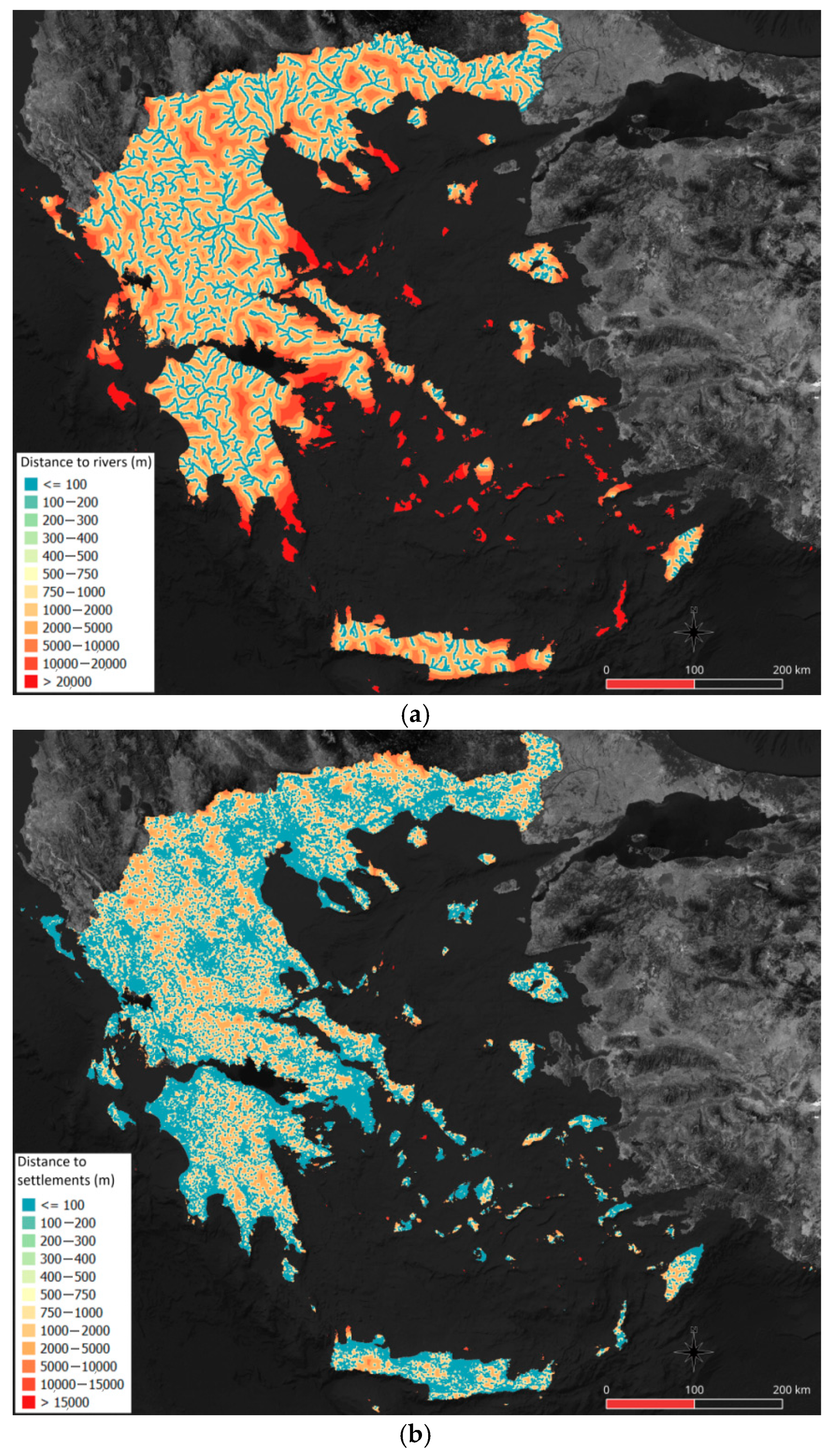
| Distance to Rivers | Rivers in Greece (vector dataset) from the geoportal of the Greek Ministry of Environment and Energy | QGIS: SAGA proximity on river dataset, reproject to EPSG 2100, resampled to 500 m |
| Distance to Settlements | Copernicus CLMS, high-resolution raster layer share of built-up (reference year 2018) [58] | QGIS: SAGA proximity on built-up dataset, reproject to EPSG 2100, resampled to 500 m |
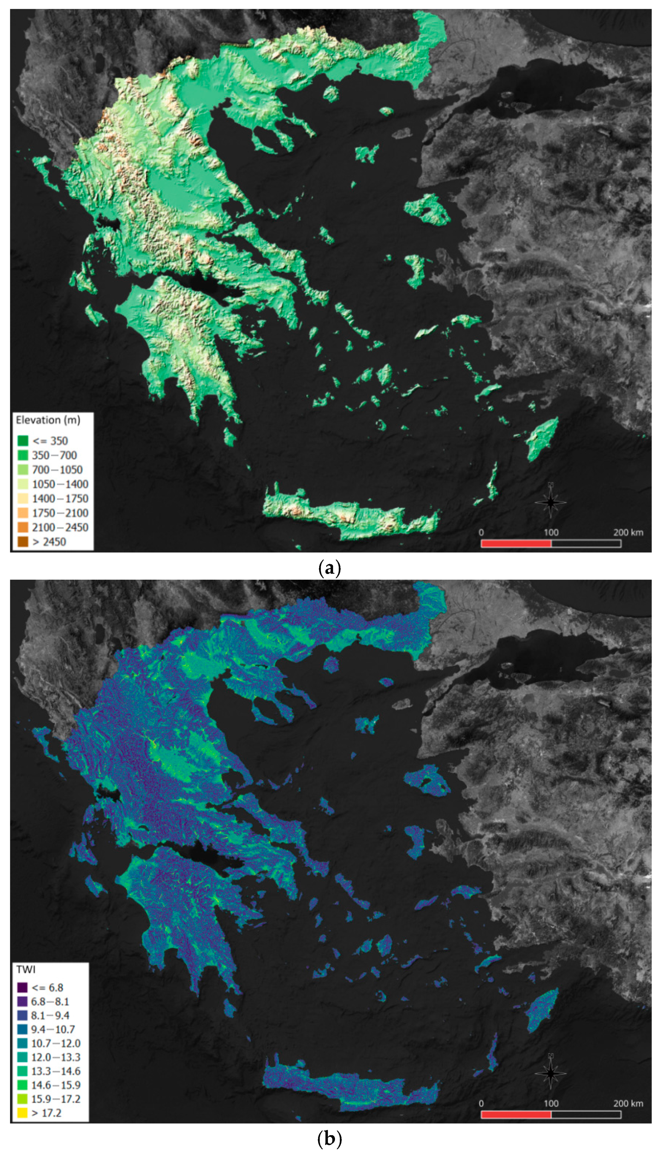
| Elevation | EU-DEM v1.1 Digital Surface Model [59] | QGIS: reproject to EPSG 2100, resampled to 500 m, mask using GR regions vector dataset |
| TWI | The derived elevation raster dataset | QGIS: SAGA terrain analysis Topographic Wetness Index algorithm, reproject to EPSG 2100, resampled to 500 m |
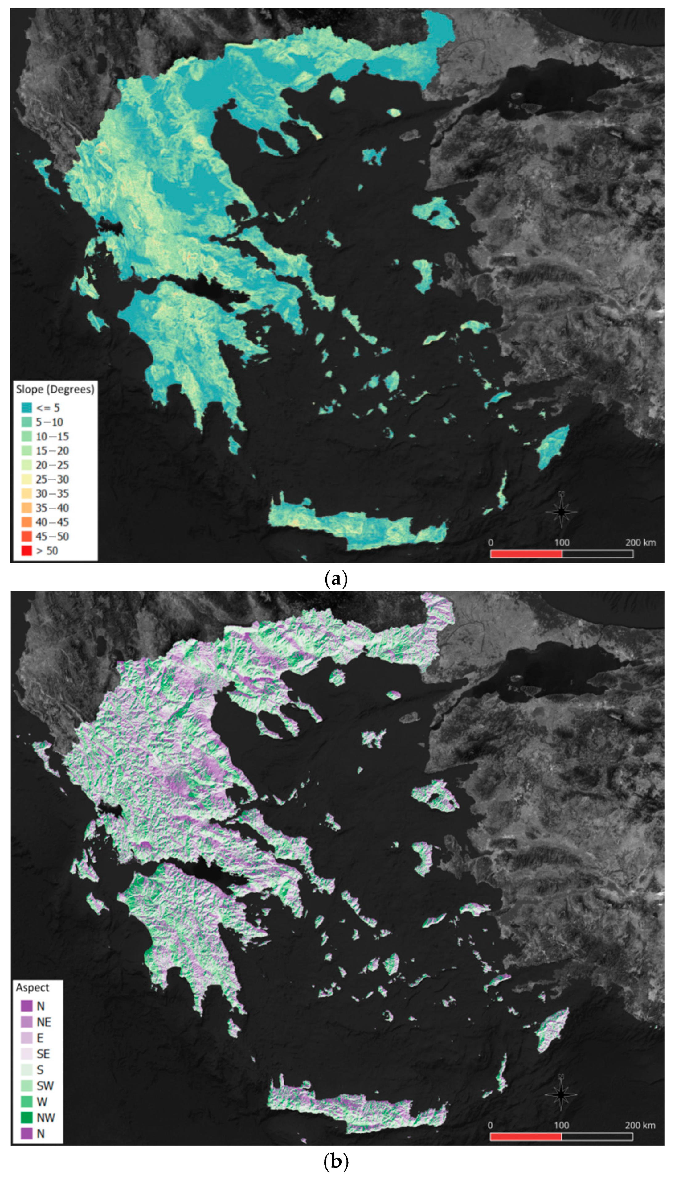
| Slope | The derived elevation raster dataset | QGIS: SAGA terrain analysis—morphometry slope, aspect, curvature algorithm, reproject to EPSG 2100, resampled to 500 m |
| Aspect | The derived elevation raster dataset | QGIS: SAGA terrain analysis—morphometry slope, aspect, curvature algorithm, reproject to EPSG 2100, resampled to 500 m |
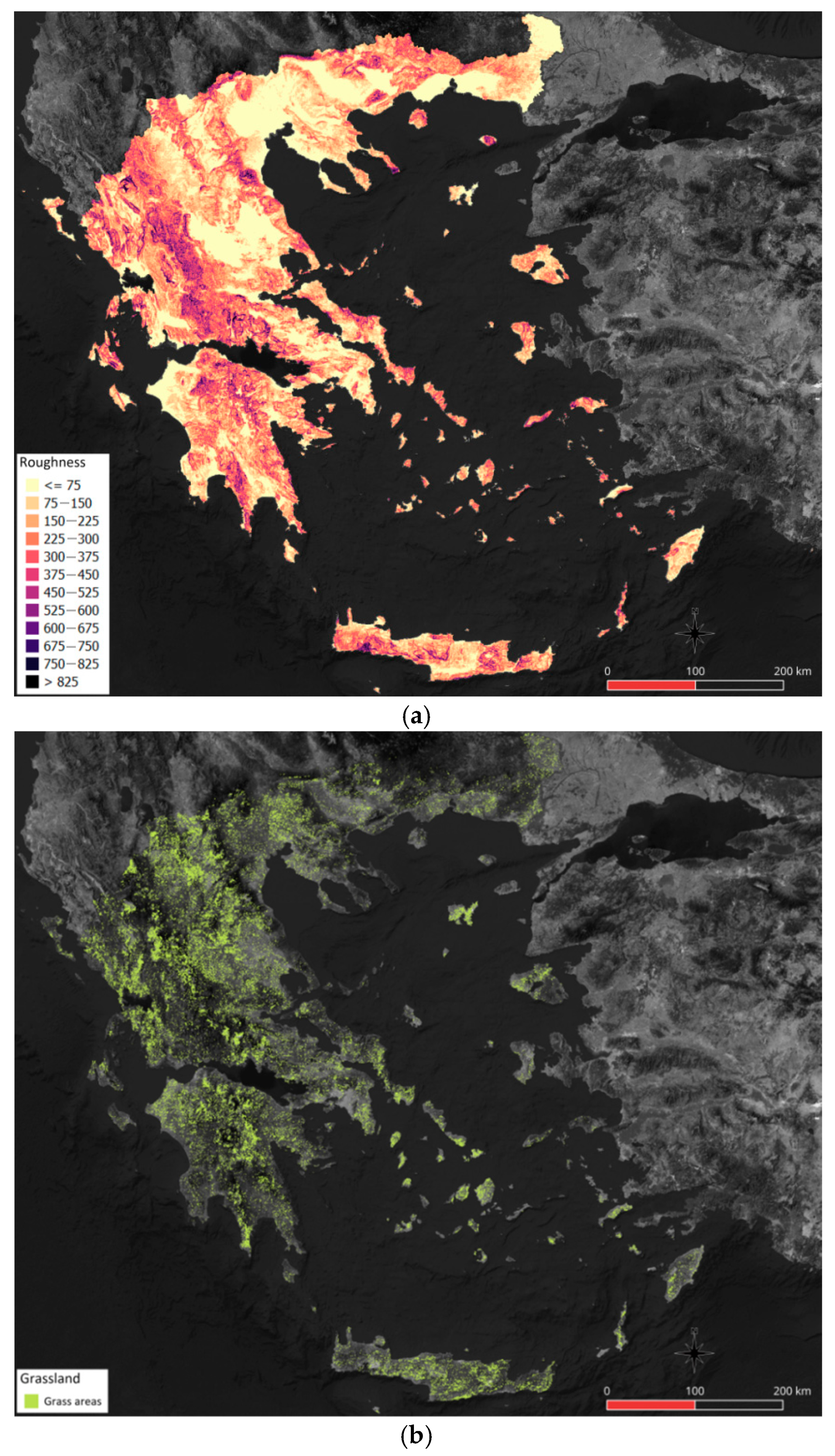
| Roughness | The derived elevation raster dataset | QGIS: GDAL roughness algorithm, reproject to EPSG 2100, resampled to 500 m |
| Grassland | Copernicus CLMS, high-resolution raster layer grassland [60] | QGIS: reproject to EPSG 2100, resampled to 500 m |
| Dominant Leaf Type | Copernicus CLMS, high-resolution raster layer dominant leaf type [61] | QGIS: reproject to EPSG 2100, resampled to 500 m |
| Number of days with very high fire danger | Copernicus C3S Climate Data Store, fire danger indicators for Europe from 1970 to 2098 derived from climate projections dataset [62] | CDO: sellonlatbox, seltime, remapbil, QGIS: reproject to EPSG 2100, resampled to 500 m, mask using GR regions vector dataset |
| Models | std-NRMSE |
|---|---|
| XGBoost | 0.8451 |
| GBM | 0.8330 |
| LightGBM | 0.8480 |
| CatBoost | 0.8147 |
| Features | XGBoost | LightGBM | GBM | CatBoost |
|---|---|---|---|---|
| Land Use | ||||
| Land use | 18.30% | 6.80% | 12.09% | 12.20% |
| Dominant Leaf Type | 0.01% | 0.01% | 0.01% | 0.01% |
| Grass | 5.59% | 1.09% | 1.00% | 1.79% |
| Land Use Sub-total | 23.90% | 7.90% | 13.10% | 14.00% |
| Topographic | ||||
| Elevation | 19.60% | 14.50% | 23.50% | 16.20% |
| Slope | 3.10% | 7.10% | 6.80% | 4.30% |
| Aspect | 2.40% | 8.00% | 3.40% | 6.80% |
| Roughness | 24.50% | 10.20% | 18.00% | 10.30% |
| Topographic Weather Index | 4.50% | 7.00% | 5.10% | 5.50% |
| Topographic Sub-total | 54.10% | 46.80% | 56.80% | 43.10% |
| Proximity | ||||
| Distance Built | 4.70% | 4.70% | 3.00% | 5.90% |
| Distance River | 5.10% | 15.60% | 7.70% | 13.00% |
| Distance Road | 3.80% | 5.10% | 3.10% | 5.30% |
| Proximity Sub-total | 13.60% | 25.40% | 13.80% | 24.20% |
| Climatic | ||||
| Fire Weather Index | 8.40% | 19.90% | 16.20% | 18.60% |
| Climate Sub-total | 8.40% | 19.90% | 16.20% | 18.60% |
Disclaimer/Publisher’s Note: The statements, opinions and data contained in all publications are solely those of the individual author(s) and contributor(s) and not of MDPI and/or the editor(s). MDPI and/or the editor(s) disclaim responsibility for any injury to people or property resulting from any ideas, methods, instructions or products referred to in the content. |
© 2025 by the authors. Licensee MDPI, Basel, Switzerland. This article is an open access article distributed under the terms and conditions of the Creative Commons Attribution (CC BY) license (https://creativecommons.org/licenses/by/4.0/).
Share and Cite
Symeonidis, P.; Vafeiadis, T.; Ioannidis, D.; Tzovaras, D. Wildfire Susceptibility Mapping in Greece Using Ensemble Machine Learning. Earth 2025, 6, 75. https://doi.org/10.3390/earth6030075
Symeonidis P, Vafeiadis T, Ioannidis D, Tzovaras D. Wildfire Susceptibility Mapping in Greece Using Ensemble Machine Learning. Earth. 2025; 6(3):75. https://doi.org/10.3390/earth6030075
Chicago/Turabian StyleSymeonidis, Panagiotis, Thanasis Vafeiadis, Dimosthenis Ioannidis, and Dimitrios Tzovaras. 2025. "Wildfire Susceptibility Mapping in Greece Using Ensemble Machine Learning" Earth 6, no. 3: 75. https://doi.org/10.3390/earth6030075
APA StyleSymeonidis, P., Vafeiadis, T., Ioannidis, D., & Tzovaras, D. (2025). Wildfire Susceptibility Mapping in Greece Using Ensemble Machine Learning. Earth, 6(3), 75. https://doi.org/10.3390/earth6030075