
The Crucial Role of Data Quality Control in Hydrochemical Studies: Reevaluating Groundwater Evolution in the Jiangsu Coastal Plain, China


Abstract
1. Introduction
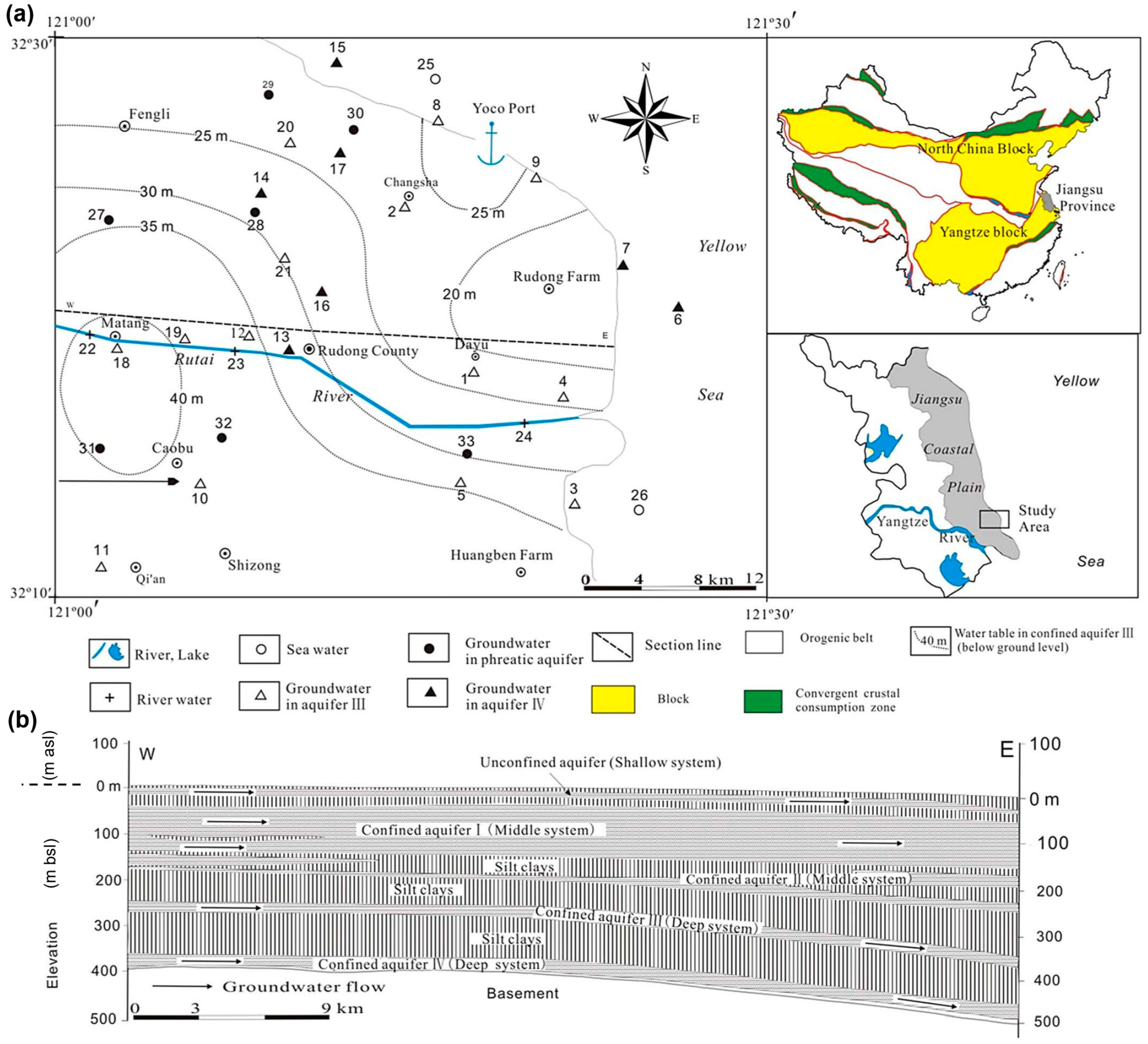
2. Study Area
3. Methodology
4. Results
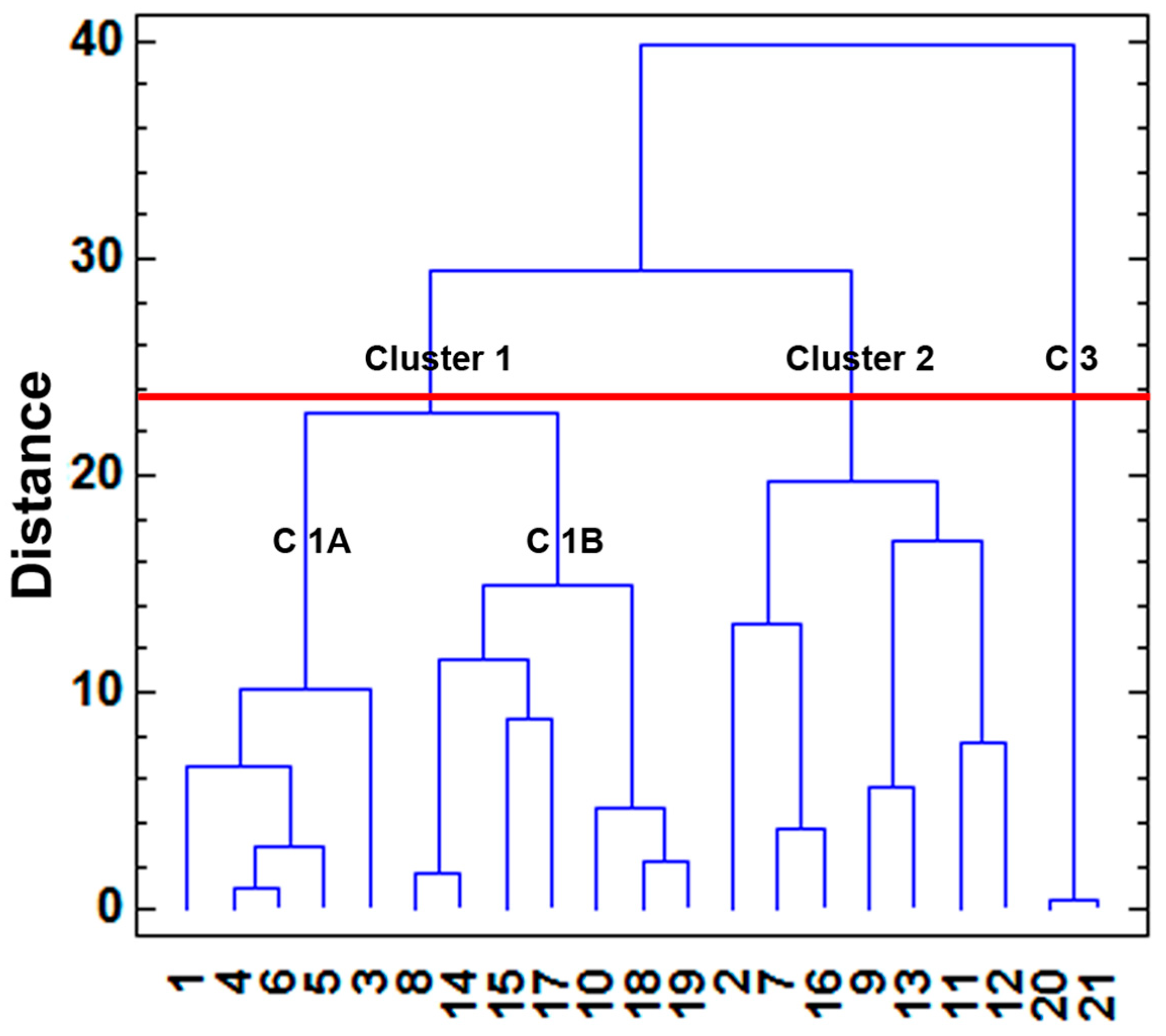
4.1. HCA
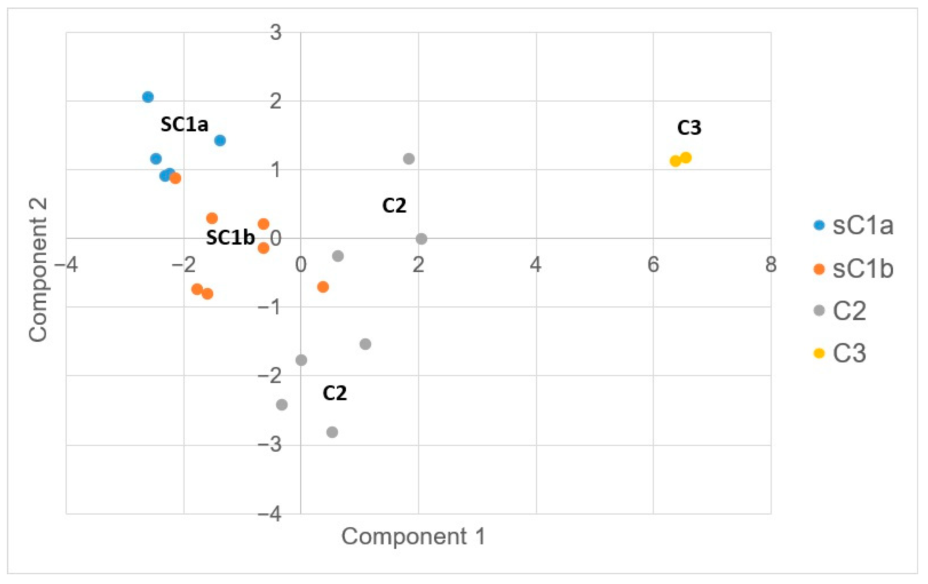
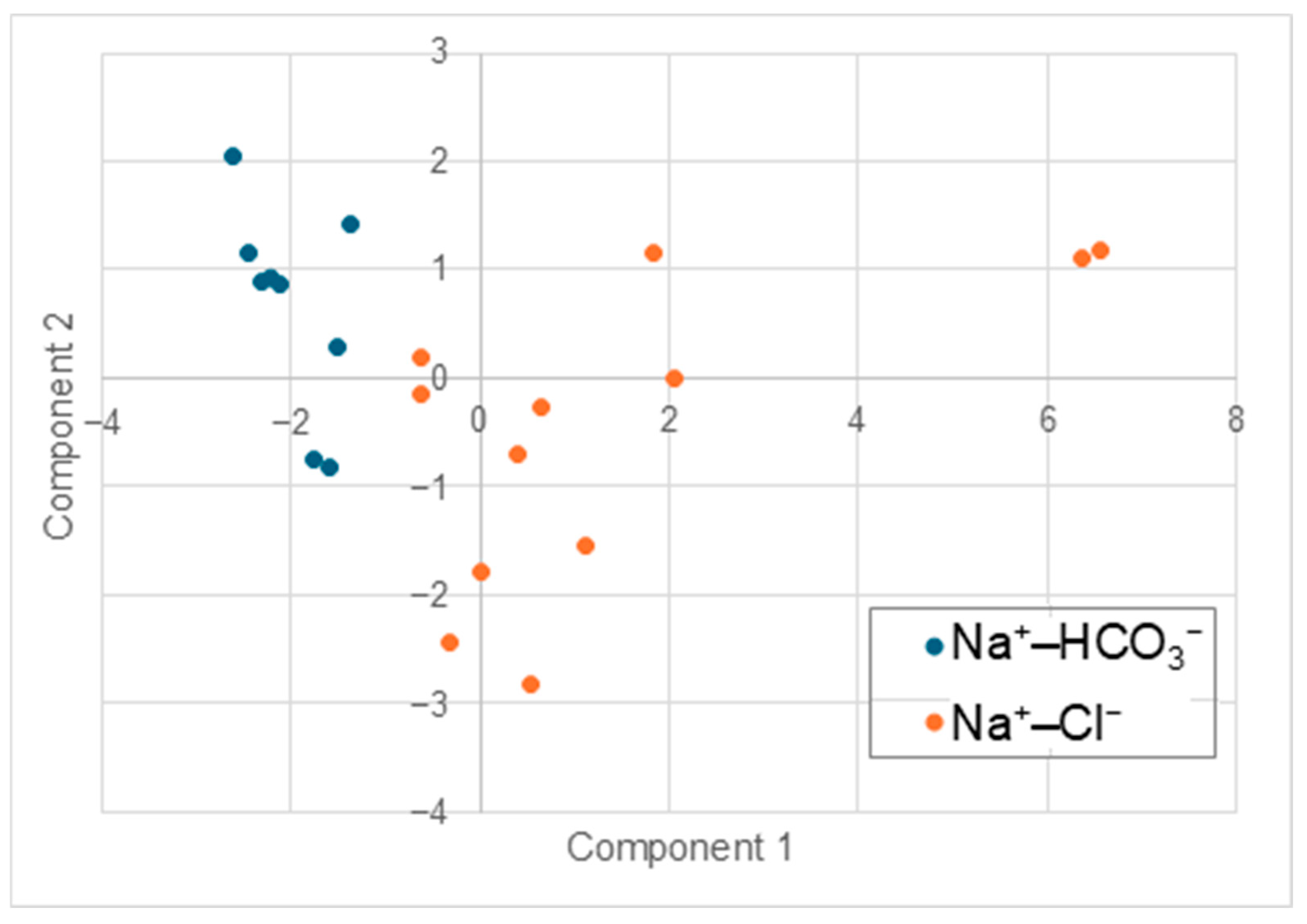
4.2. PCA
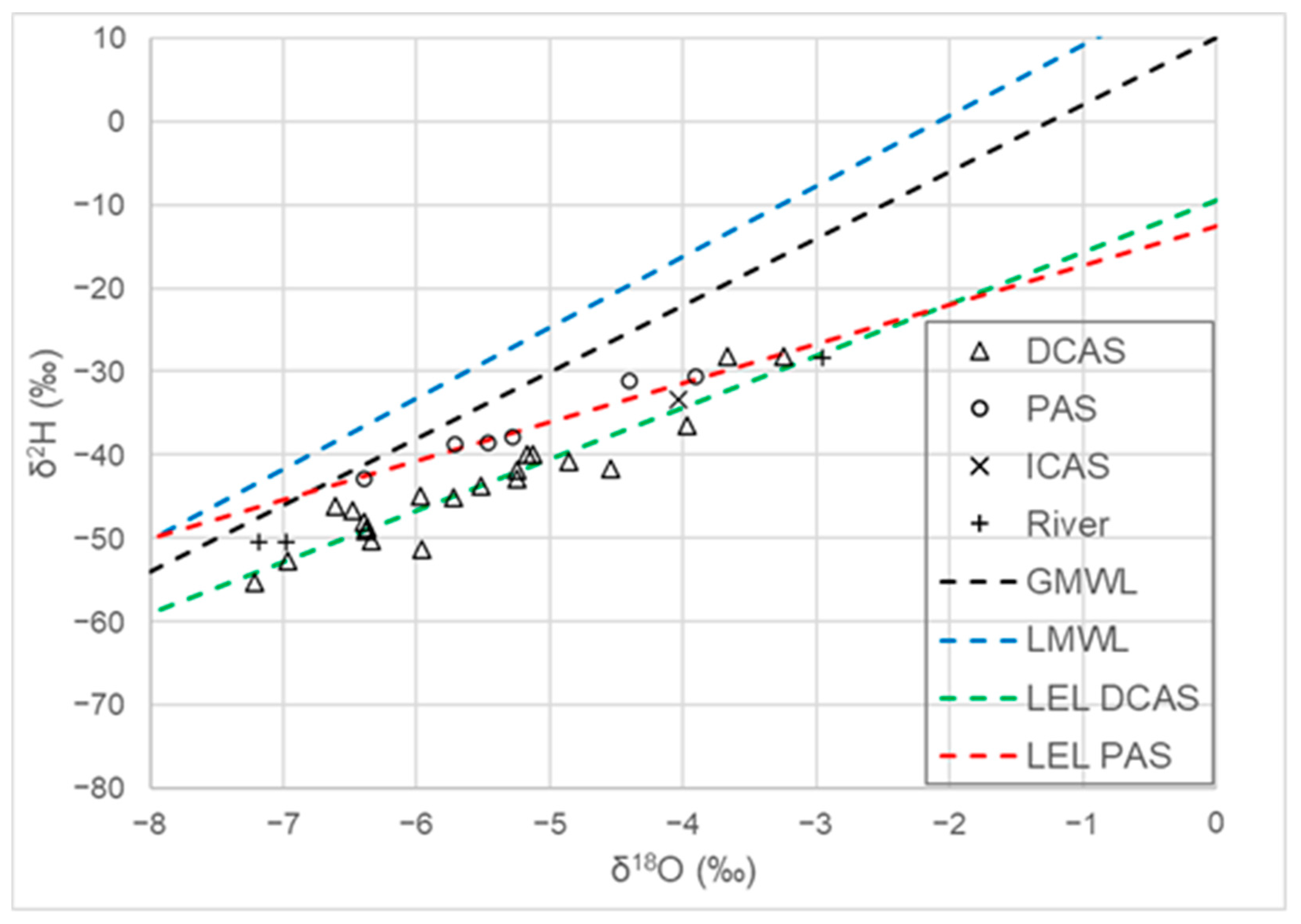
4.3. Environmental Isotopes
4.4. Radioactive Isotopes
5. Discussion: The Processes Affecting Groundwater Evolution in the Jiangsu Coastal Plain
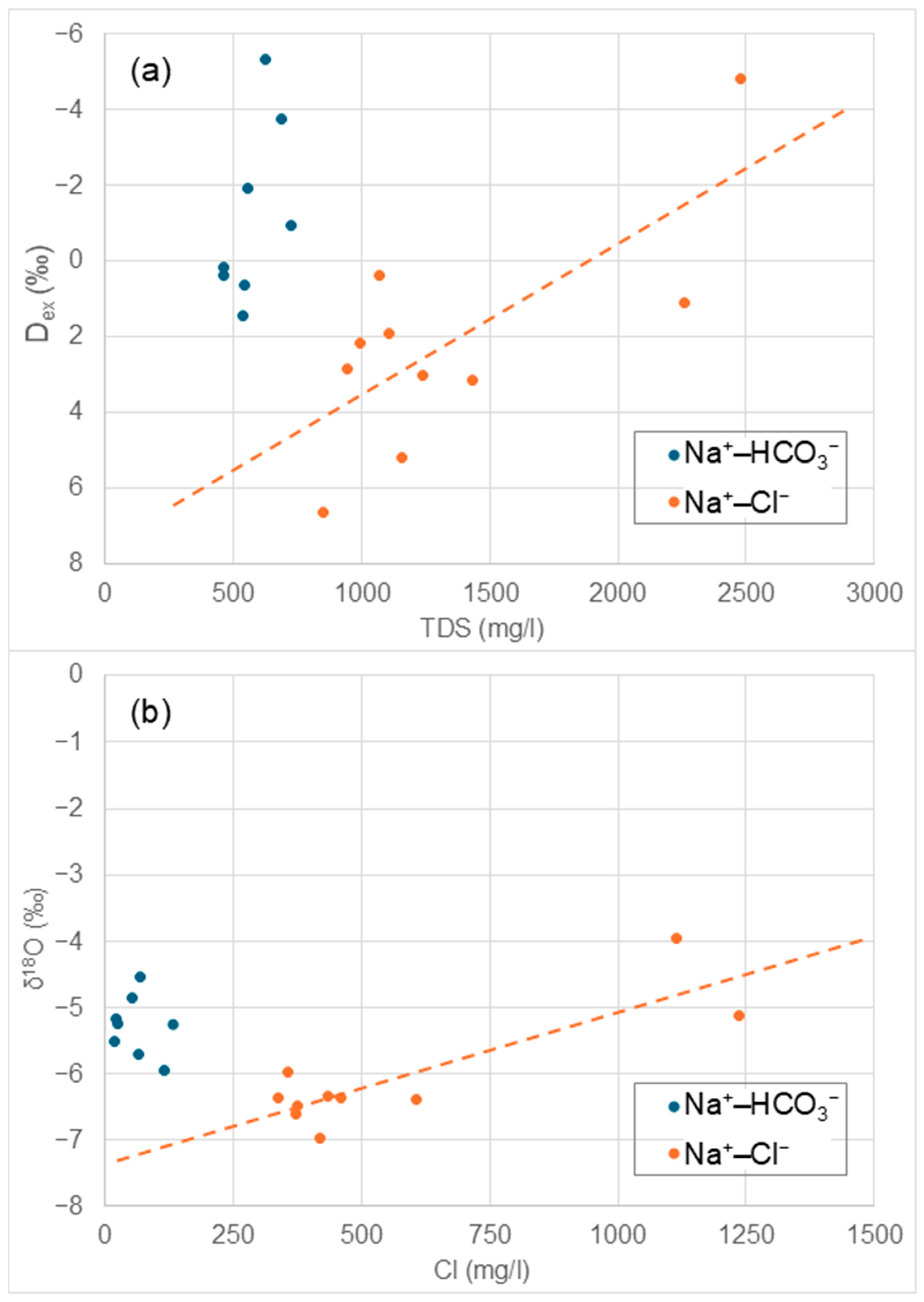
5.1. Evaporation Processes
5.2. Water–Rock Interaction in the DCAS
5.3. Seawater Intrusion in the DCAS
5.4. Residence Times in the DCAS
6. Conclusions
- A QA/QC analysis identified anomalous Fe and Mn concentrations in five samples, which were inconsistent with TDS values. As a result, the Fe and Mn concentrations were discarded for these samples. Consequently, these elements were not included as input data for HCA and PCA, as reliable information was not available for all samples. This underscores the importance of conducting thorough QA/QC procedures to ensure data integrity.
- Charge Balance Error (CBE) is the tool used most usually for laboratory data QA/QC. Even though it is an excellent first approach, it is advisable to use it in combination with additional QA/QC techniques. In the analyzed dataset in this study, CBE validated samples that were later discarded for anomalous Fe and Mn concentrations. In order to take better advantage of CBE it is more helpful to evaluate it using it all ions and not only major ones.
- Three key processes were identified as drivers of hydrochemical variations in the deep groundwater of the Jiangsu Coastal Plain: water–rock interaction, evaporation, and seawater intrusion. Water–rock interaction was found to be the dominant hydrochemical process influencing Na+–HCO3− waters (freshwater). Evaporation was determined to be the primary process responsible for mineralization in Na+–Cl− waters (brackish water).
- The occurrence of seawater intrusion was demonstrated in two wells (20 and 21, classified as saline waters). This conclusion is based on a combination of a statistical assessment (HCA and PCA) of hydrochemical data and environmental isotopes (δ2H and δ18O plots, along with Dex values).
- Seawater intrusion was identified as affecting only Aquifer III of the DCAS. Given the location of the two affected wells, where groundwater flows inland from the shoreline towards drawdown cones induced by groundwater extraction, this process may be considered ongoing. However, this finding remains inconclusive due to contradictory radiogenic isotope data. It is advisable to further study the DCAS, including a more comprehensive analytical suite (including most dissolved anions and cations) plus additional isotopes like 87Sr/86Sr that may help to better refine this process.
- Based on these observations, it is highly advisable to account for seawater intrusion in groundwater management strategies for the area. Step drawdowns are recorded in the Matang area. Hence, a detailed monitoring program for groundwater levels and water quality using telemetry for live data and probably reducing extractions are good first steps.
- Residence time estimations revealed contradictions in seven samples, representing 33% of the dataset. These samples contained measurable amounts of 3H (with TU values above the detection limit), suggesting a recharge age of less than 60 years. However, the same samples were assigned corrected 14C ages ranging from 17,000 to 23,000 years BP. Due to this inconsistency, paleoclimatic reconstructions based on these data cannot be deemed reliable.
Author Contributions
Funding
Data Availability Statement
Acknowledgments
Conflicts of Interest
Abbreviations
| DCAS | Deep Confined Aquifer System |
| QA/QC | Quality Assurance and Quality Control |
| HCA | Hierarchical Cluster Analysis |
| PCA | Principal Component Analysis |
| PAS | Phreatic Aquifer System |
| ICAS | Intermediate Confined Aquifer System |
| TDS | Total Dissolved Solids |
| Dex | Deuterium Excess |
| GMWL | Global Meteoric Water Line |
| LMWL | Local Meteoric Water Line |
| LEL | Local Evaporation Line |
| pmc | Percentage of Modern Carbon |
| BP | Before Present |
| r | Correlation Coefficient |
| CBE | Charge Balance Error |
| m bgl | Meters Below Ground Level |
References
- Freeze, R.A.; Cherry, J.A. Groundwater; Prentice-Hall: Englewood Cliffs, NJ, USA, 1979. [Google Scholar]
- Fritz, S.J. A survey of charge-balance errors on published analyses of potable ground and surface waters. Groundwater 1994, 32, 539–546. [Google Scholar] [CrossRef]
- Li, X.; Wu, H.; Qian, H.; Gao, Y. Groundwater chemistry regulated by hydrochemical processes and geological structures: A case study in Tongchuan, China. Water 2018, 10, 338. [Google Scholar] [CrossRef]
- Katz, B.; Collins, J. Evaluation of Chemical Data from Selected Sites in the Surface-Water Ambient Monitoring Program (SWAMP) in Florida; Open-File Report 98–559; US Geological Survey: Reston, VA, USA, 1998; 51p. [Google Scholar]
- Hem, J.D. Study and Interpretation of the Chemical Characteristics of Natural Water; U.S. Geological Survey: Washington, DC, USA, 1985. [Google Scholar]
- Hounslow, A.W. Water Quality Data; CRC Press: Boca Raton, FL, USA, 1995; ISBN 9780203734117. [Google Scholar]
- Güler, C.; Thyne, G.D.; McCray, J.E.; Turner, K.A. Evaluation of graphical and multivariate statistical methods for classification of water chemistry data. Hydrogeol. J. 2002, 10, 455–474. [Google Scholar] [CrossRef]
- Guggenmos, M.R.; Daughney, C.J.; Jackson, B.M.; Morgenstern, U. Regional-scale identification of groundwater-surface water interaction using hydrochemistry and multivariate statistical methods, Wairarapa Valley, New Zealand. Hydrol. Earth Syst. Sci. 2011, 15, 3383–3398. [Google Scholar] [CrossRef]
- Moya, C.E.; Raiber, M.; Taulis, M.; Cox, M.E. Hydrochemical evolution and groundwater flow processes in the Galilee and Eromanga basins, Great Artesian Basin, Australia: A multivariate statistical approach. Sci. Total Environ. 2015, 508, 411–426. [Google Scholar] [CrossRef]
- Xu, N.; Gong, J.; Yang, G. Using environmental isotopes along with major hydro-geochemical compositions to assess deep groundwater formation and evolution in eastern coastal China. J. Contam. Hydrol. 2018, 208, 1–9. [Google Scholar] [CrossRef]
- Ma, Y.Y.; Lu, Y.Q.; Zhang, L. Evolvement of spatial pattern of population with data at county level in Jiangsu Province. Prog. Geogr. 2012, 31, 167–175. [Google Scholar]
- Bao, J.; Gao, S.; Ge, J. Coastal engineering evolution in low-lying areas and adaptation practice since the eleventh century, Jiangsu Province, China. Clim. Change 2020, 162, 799–817. [Google Scholar] [CrossRef]
- Ferguson, G.; Gleeson, T. Vulnerability of coastal aquifers to groundwater use and climate change. Nat. Clim. Change 2012, 2, 342–345. [Google Scholar] [CrossRef]
- Alfarrah, N.; Walraevens, K. Groundwater Overexploitation and Seawater Intrusion in Coastal Areas of Arid and Semi-Arid Regions. Water 2018, 10, 143. [Google Scholar] [CrossRef]
- Hussain, M.S.; Abd-Elhamid, H.F.; Javadi, A.A.; Sherif, M.M. Management of Seawater Intrusion in Coastal Aquifers: A Review. Water 2019, 11, 2467. [Google Scholar] [CrossRef]
- Dey, S.; Prakash, O. Management of Saltwater Intrusion in Coastal Aquifers: An Overview of Recent Advances. In Environmental Processes and Management; Singh, R.M., Shukla, P., Singh, P., Eds.; Springer International Publishing: Cham, Germany, 2020; pp. 321–344. ISBN 978-3-030-38151-6. [Google Scholar]
- Zhang, Y.; Xue, Y.-Q.; Wu, J.-C.; Shi, X.-Q.; Yu, J. Excessive groundwater withdrawal and resultant land subsidence in the Su-Xi-Chang area, China. Environ. Earth Sci. 2010, 61, 1135–1143. [Google Scholar] [CrossRef]
- Huang, F.; Wang, G.H.; Yang, Y.Y.; Wang, C.B. Overexploitation status of groundwater and induced geological hazards in China. Nat. Hazards 2014, 73, 727–741. [Google Scholar] [CrossRef]
- Shi, L.; Jiao, J.J. Seawater intrusion and coastal aquifer management in China: A review. Environ. Earth Sci. 2014, 72, 2811–2819. [Google Scholar] [CrossRef]
- Scheihing, K.W.; Fraser, C.M.; Vargas, C.R.; Kukurić, N.; Lictevout, E. A review of current capacity development practice for fostering groundwater sustainability. Groundw. Sustain. Dev. 2022, 19, 100823. [Google Scholar] [CrossRef]
- Shi, X.; Jiang, F.; Feng, Z.; Yao, B.; Xu, H.; Wu, J. Characterization of the regional groundwater quality evolution in the North Plain of Jiangsu Province, China. Environ. Earth Sci. 2015, 74, 5587–5604. [Google Scholar] [CrossRef]
- Dansgaard, W. Stable isotopes in precipitation. Tellus A Dyn. Meteorol. Oceanogr. 1964, 16, 436. [Google Scholar] [CrossRef]
- Mao, C.; Tan, H.; Song, Y.; Rao, W. Evolution of groundwater chemistry in coastal aquifers of the Jiangsu, east China: Insights from a multi-isotope (δ2H, δ18O, 87Sr/86Sr, and δ11B) approach. J. Contam. Hydrol. 2020, 235, 103730. [Google Scholar] [CrossRef]
- Davis, J.C. Statistics and Data Analysis in Geology, 3rd ed.; Wiley: New Delhi, India, 2015; ISBN 9788126530083. [Google Scholar]
- Moeck, C.; Radny, D.; Borer, P.; Rothardt, J.; Auckenthaler, A.; Berg, M.; Schirmer, M. Multicomponent statistical analysis to identify flow and transport processes in a highly-complex environment. J. Hydrol. 2016, 542, 437–449. [Google Scholar] [CrossRef]
- Raiber, M.; Lewis, S.; Cendón, D.I.; Cui, T.; Cox, M.E.; Gilfedder, M.; Rassam, D.W. Significance of the connection between bedrock, alluvium and streams: A spatial and temporal hydrogeological and hydrogeochemical assessment from Queensland, Australia. J. Hydrol. 2019, 569, 666–684. [Google Scholar] [CrossRef]
- Wold, S.; Esbensen, K.; Geladi, P. Principal component analysis. Chemom. Intell. Lab. Syst. 1987, 2, 37–52. [Google Scholar] [CrossRef]
- Stetzenbach, K.J.; Farnham, I.M.; Hodge, V.F.; Johannesson, K.H. Using multivariate statistical analysis of groundwater major cation and trace element concentrations to evaluate groundwater flow in a regional aquifer. Hydrol. Process. 1999, 13, 2655–2673. [Google Scholar] [CrossRef]
- O’Shea, B.; Jankowski, J. Detecting subtle hydrochemical anomalies with multivariate statistics: An example from ‘homogeneous’ groundwaters in the Great Artesian Basin, Australia. Hydrol. Process. 2006, 20, 4317–4333. [Google Scholar] [CrossRef]
- Kaiser, H.F. The Application of Electronic Computers to Factor Analysis. Educ. Psychol. Meas. 1960, 20, 141–151. [Google Scholar] [CrossRef]
- Craig, H. Isotopic Variations in Meteoric Waters. Science 1961, 133, 1702–1703. [Google Scholar] [CrossRef] [PubMed]
- Xu, N.; Liu, H.; Wei, F. Study on the environmental isotope compositions and their evolution in groundwater of Yoco port in Jiangsu Province, China. Acta Sci. Circumst. 2015, 35, 3862–3871. [Google Scholar]
- Scheihing, K.; Moya, C.; Struck, U.; Lictevout, E.; Tröger, U. Reassessing Hydrological Processes That Control Stable Isotope Tracers in Groundwater of the Atacama Desert (Northern Chile). Hydrology 2018, 5, 3. [Google Scholar] [CrossRef]
- Kong, Y.; Wang, K.; Li, J.; Pang, Z. Stable Isotopes of Precipitation in China: A Consideration of Moisture Sources. Water 2019, 11, 1239. [Google Scholar] [CrossRef]
- Huang, T.; Pang, Z. The role of deuterium excess in determining the water salinisation mechanism: A case study of the arid Tarim River Basin, NW China. Appl. Geochem. 2012, 27, 2382–2388. [Google Scholar] [CrossRef]
- Cartwright, I.; Morgenstern, U. Using tritium and other geochemical tracers to address the “old water paradox” in headwater catchments. J. Hydrol. 2018, 563, 13–21. [Google Scholar] [CrossRef]
- Clark, I.D.; Fritz, P. Environmental Isotopes in Hydrogeology; CRC Press: Boca Raton, FL, USA, 2013; ISBN 9780429069574. [Google Scholar]
- Cartwright, I.; Weaver, T.R.; Cendón, D.I.; Fifield, L.K.; Tweed, S.O.; Petrides, B.; Swane, I. Constraining groundwater flow, residence times, inter-aquifer mixing, and aquifer properties using environmental isotopes in the southeast Murray Basin, Australia. Appl. Geochem. 2012, 27, 1698–1709. [Google Scholar] [CrossRef]
- Moya, C.E.; Raiber, M.; Taulis, M.; Cox, M.E. Using environmental isotopes and dissolved methane concentrations to constrain hydrochemical processes and inter-aquifer mixing in the Galilee and Eromanga Basins, Great Artesian Basin, Australia. J. Hydrol. 2016, 539, 304–318. [Google Scholar] [CrossRef]
- Taulis, M.; Milke, M. Chemical variability of groundwater samples collected from a coal seam gas exploration well, Maramarua, New Zealand. Water Res. 2013, 47, 1021–1034. [Google Scholar] [CrossRef] [PubMed]
- Li, J.; Liang, X.; Zhang, Y.; Liu, Y.; Chen, N.; Abubakari, A.; Jin, M. Salinization of porewater in a multiple aquitard-aquifer system in Jiangsu coastal plain, China. Hydrogeol. J. 2017, 25, 2377–2390. [Google Scholar] [CrossRef]
- Suckow, A. The age of groundwater–Definitions, models and why we do not need this term. Appl. Geochem. 2014, 50, 222–230. [Google Scholar] [CrossRef]
- Suckow, A.; Deslandes, A.; Raiber, M.; Taylor, A.R.; Davies, P.; Gerber, C.; Leaney, F. Reconciling contradictory environmental tracer ages in multi-tracer studies to characterize the aquifer and quantify deep groundwater flow: An example from the Hutton Sandstone, Great Artesian Basin, Australia. Hydrogeol. J. 2020, 28, 75–87. [Google Scholar] [CrossRef]


| ID | Aquifer | pH | T | TDS | Cl− | HCO3− | SO42− | Ca2+ | Mg2+ | Na+ | K+ | H2SiO3 | Fe | Mn | CBE | TDScalc | TDScalc * |
|---|---|---|---|---|---|---|---|---|---|---|---|---|---|---|---|---|---|
| (°C) | mg/L | mg/L | mg/L | mg/L | mg/L | mg/L | mg/L | mg/L | mg/L | mg/L | mg/L | % | mg/L | mg/L | |||
| 1 | III | 7.9 | 19 | 723.3 | 129.8 | 541 | 3.9 | 83.9 | 37.5 | 112.7 | 2.3 | 35.2 | 1.8 | 0.1 | −0.4 | 673 | 671 |
| 2 | III | 7.9 | 17.8 | 2479.3 | 1113.3 | 526.3 | 94.4 | 236.3 | 94.7 | 462 | 5.8 | 24.2 | 13.2 | 0.2 | −2.2 | 2303 | 2290 |
| 3 | III | 7.4 | 24.5 | 462 | 25.2 | 478 | 4 | 64.1 | 26.1 | 82.2 | 1.5 | 33.8 | 1.5 | 0 | 0.3 | 473 | 472 |
| 4 | III | 7.7 | 23.8 | 464 | 18.9 | 459 | 3.7 | 61 | 26.7 | 78.1 | 1.6 | 31.1 | 0.5 | 0 | 0.5 | 447 | 447 |
| 5 | III | 7.9 | 25.1 | 534 | 22.1 | 466 | 3.7 | 64 | 26.3 | 78.7 | 1.4 | 33.4 | 0.9 | 0 | 0.5 | 460 | 459 |
| 6 | IV | 7.7 | 23.8 | 542 | 63 | 490 | 3.8 | 48.1 | 20.6 | 140 | 1.3 | 28 | 0.9 | 0.1 | 0.3 | 547 | 546 |
| 7 | IV | 7.7 | 24.8 | 2262 | 1236 | 301 | 76.3 | 170 | 61.4 | 587 | 10.1 | 22.1 | 1.4 | 0.2 | −2.1 | 2313 | 2311 |
| 8 | III | 7.8 | 22.9 | 942 | 357 | 407 | 15.1 | 50 | 23.6 | 278 | 2.6 | 26.5 | 1.8 | 0.1 | −0.5 | 955 | 953 |
| 9 | III | 8.1 | 20.3 | 852 | 372 | 286 | 19.7 | 31.9 | 20.8 | 286 | 2.4 | 15.2 | 3.6 | 0.1 | 0.2 | 892 | 889 |
| 10 | III | 7.9 | 23 | 558 | 51.3 | 502 | 7.2 | 50.9 | 24 | 135 | 1.6 | 13.4 | 0.2 | 0.2 | 0.6 | 531 | 530 |
| 11 | III | 7.8 | 24.5 | 1156 | 375 | 313 | 209 | 115 | 49.3 | 236 | 5 | 11.4 | 2 | 0.1 | 0.1 | 1157 | 1155 |
| 12 | III | 7.7 | 24.9 | 1106 | 458 | 295 | 7.1 | 72.1 | 35.1 | 263 | 3.4 | 10.6 | 0 | 0.1 | 0.1 | 994 | 994 |
| 13 | IV | 8.3 | 21.1 | 1066 | 433 | 301 | 11.2 | 69.6 | 33.2 | 255 | 5.2 | 12.1 | 0 | 0 | 0.1 | 967 | 967 |
| 14 | IV | 7.7 | 22 | 992 | 338 | 419 | 12.7 | 63.1 | 24 | 250 | 2.5 | 18.1 | 775 | 16.4 | −0.6 | 1706 | 914 |
| 15 | IV | 8 | 19.6 | 622 | 68.1 | 475 | 38.8 | 20.9 | 11.7 | 190 | 2.6 | 19.5 | 725 | 15.6 | −0.2 | 1326 | 585 |
| 16 | IV | 7.8 | 29 | 1432 | 606 | 304 | 18.3 | 102 | 49.8 | 287 | 4.2 | 23.8 | 2010 | 61.3 | −0.7 | 3312 | 1241 |
| 17 | IV | 8.1 | 34.3 | 1238 | 418 | 413 | 58.5 | 55.6 | 33.7 | 316 | 4.1 | 21.3 | 2120 | 66.5 | −0.4 | 3297 | 1110 |
| 18 | III | 7.8 | 23.7 | 688 | 114 | 493 | 8.4 | 53.5 | 26.3 | 155 | 1.6 | 21.1 | 3120 | 89.5 | 0.1 | 3832 | 622 |
| 19 | III | 7.8 | 24.3 | 608 | 29.8 | 621 | 8.8 | 45.7 | 21.6 | 166 | 1.5 | 22.2 | 730 | 55.7 | 0.1 | 1387 | 601 |
| 20 | III | 8 | 18.2 | 19,962 | 9608 | 401 | 1190 | 887 | 687 | 4438 | 37.4 | 23.3 | 49 | 0.5 | −7.6 | 17,117 | 17,068 |
| 21 | III | 7.9 | 18.8 | 19,718 | 9740 | 382 | 1203 | 533 | 534 | 5454 | 44.7 | 23.7 | 130 | 0.3 | 2.9 | 17,851 | 17,720 |
| ID | Aquifer System | Membership | δ2H | δ18O | Dex | 3H | 14C Based Age | 14C Activity |
|---|---|---|---|---|---|---|---|---|
| (‰) | (‰) | (‰) | TU | Years BP | pmc | |||
| 1 | DCAS | Aquifer III | −42.94 | −5.25 | −0.94 | <2 | 17,940 ± 140 | 9.70 |
| 2 | DCAS | Aquifer III | −36.58 | −3.97 | −4.82 | <2 | 11,270 ± 110 | 21.75 |
| 3 | DCAS | Aquifer III | −41.84 | −5.25 | 0.16 | 15.8 | 18,490 ± 340 | 9.08 |
| 4 | DCAS | Aquifer III | −43.8 | −5.52 | 0.36 | <2 | 16,100 ± 100 | 12.12 |
| 5 | DCAS | Aquifer III | −39.92 | −5.17 | 1.44 | <2 | 17,260 ± 100 | 10.54 |
| 6 | DCAS | Aquifer IV | −45.13 | −5.72 | 0.63 | <2 | 18,200 ± 130 | 9.40 |
| 7 | DCAS | Aquifer IV | −39.92 | −5.13 | 1.12 | <2 | 16,140 ± 130 | 12.07 |
| 8 | DCAS | Aquifer III | −44.9 | −5.97 | 2.86 | <2 | 26,140 ± 300 | 3.60 |
| 9 | DCAS | Aquifer III | −46.25 | −6.61 | 6.63 | 2.47 | 22,950 ± 510 | 5.29 |
| 10 | DCAS | Aquifer III | −40.79 | −4.86 | −1.91 | <2 | 20,380 ± 280 | 7.22 |
| 11 | DCAS | Aquifer III | −46.66 | −6.48 | 5.18 | <2 | 24,880 ± 260 | 4.19 |
| 12 | DCAS | Aquifer III | −49.12 | −6.38 | 1.92 | <2 | 22,150 ± 250 | 5.83 |
| 13 | DCAS | Aquifer IV | −50.33 | −6.34 | 0.39 | <2 | 18,870 ± 230 | 8.67 |
| 14 | DCAS | Aquifer IV | −48.8 | −6.37 | 2.16 | 6.94 | 22,310 ± 280 | 5.72 |
| 15 | DCAS | Aquifer IV | −55.31 | −7.22 | 2.45 | 5.31 | 16,900 ± 230 | 11.01 |
| 16 | DCAS | Aquifer IV | −48.05 | −6.4 | 3.15 | 8.7 | 19,540 ± 180 | 8.00 |
| 17 | DCAS | Aquifer IV | −52.76 | −6.97 | 3 | <2 | 25,890 ± 300 | 3.71 |
| 18 | DCAS | Aquifer III | −41.64 | −4.54 | −5.32 | 13.3 | 22,490 ± 170 | 5.60 |
| 19 | DCAS | Aquifer III | −51.42 | −5.96 | −3.74 | 12 | 18,600 ± 170 | 8.96 |
| 20 | DCAS | Aquifer III | −28.2 | −3.67 | 1.16 | <2 | 7410 ± 800 | 34.69 |
| 21 | DCAS | Aquifer III | −28.15 | −3.25 | −2.15 | <2 | 9370 ± 80 | 27.36 |
| 22 | None | River | −50.45 | −7.18 | 6.99 | - | - | |
| 23 | None | River | −50.43 | −6.98 | 5.41 | - | - | |
| 24 | None | River | −28.35 | −2.96 | −4.67 | - | - | |
| 25 | None | Sea | −6.32 | −0.56 | −1.84 | - | - | |
| 26 | None | Sea | −14.52 | −1.73 | −0.68 | - | - | |
| 27 | PAS | Phreatic Aquifer | −38.67 | −5.71 | 7.01 | - | - | |
| 28 | PAS | Phreatic Aquifer | −31.13 | −4.4 | 4.07 | - | - | |
| 29 | PAS | Phreatic Aquifer | −30.69 | −3.91 | 0.59 | - | - | |
| 30 | ICAS | Aquifer I | −33.37 | −4.04 | −1.05 | - | - | |
| 31 | PAS | Phreatic Aquifer | −42.83 | −6.39 | 8.29 | - | - | |
| 32 | PAS | Phreatic Aquifer | −37.9 | −5.28 | 4.34 | - | - | |
| 33 | PAS | Phreatic Aquifer | −38.63 | −5.46 | 5.05 | - | - |
| Methodology Steps and Results | This Study | Xu et al. [10] |
|---|---|---|
| Data QA/QC before statistical analysis | Yes | No |
| Dataset log-transformation and/or normality test | Yes | No |
| Used anomalous Fe and Mn data in statistical process | No | Yes |
| HCA linkage method | Ward | |
| HCA measure of similarity | Euclidean distance | |
| Number of identified clusters | 3 | 4 |
| Number of significant components identified (Eigenvalue > 1) | 2 | 3 |
| Cluster | pH | TDS | Cl− | HCO3− | SO42− | Ca2+ | Mg2+ | Na+ | K+ | H2SiO3 | Water Type |
|---|---|---|---|---|---|---|---|---|---|---|---|
| mg/L | mg/L | mg/L | mg/L | mg/L | mg/L | mg/L | mg/L | mg/L | |||
| C1 | 7.81 | 698 | 136.3 | 480.3 | 14.1 | 55.1 | 25.2 | 165.1 | 2.1 | 25.3 | Na-HCO3 |
| sC1a | 7.72 | 545 | 51.8 | 486.8 | 3.8 | 64.2 | 27.4 | 98.3 | 1.6 | 32.3 | Na-HCO3 |
| sC1b | 7.88 | 784 | 169.9 | 487.2 | 22.4 | 48.3 | 23.6 | 202.0 | 2.3 | 19.3 | Na-HCO3 |
| C2 | 7.9 | 1479 | 656.2 | 332.3 | 62.3 | 113.8 | 49.2 | 339.4 | 5.2 | 17.1 | Na-Cl |
| C3 | 7.95 | 19840 | 9674 | 391.5 | 1196.5 | 710 | 610.5 | 4946 | 41.1 | 23.5 | Na-Cl |
| Variable | PCA1 | PCA2 |
|---|---|---|
| pH | 0.12 | −0.41 |
| Log TDS | 0.38 | 0.10 |
| Log Cl− | 0.37 | −0.11 |
| Log HCO3− | −0.16 | 0.52 |
| Log SO42− | 0.36 | −0.02 |
| Log Ca2+ | 0.35 | 0.26 |
| Log Mg2+ | 0.36 | 0.21 |
| Log Na+ | 0.38 | 0.02 |
| Log K+ | 0.38 | 0.01 |
| Log H2SiO3 | −0.06 | 0.65 |
| Eigenvalue | 6.58 | 1.76 |
| Percentage of explained variance | 65.8 | 17.6 |
| Cumulative percentage of variance | 65.8 | 83.4 |
Disclaimer/Publisher’s Note: The statements, opinions and data contained in all publications are solely those of the individual author(s) and contributor(s) and not of MDPI and/or the editor(s). MDPI and/or the editor(s) disclaim responsibility for any injury to people or property resulting from any ideas, methods, instructions or products referred to in the content. |
© 2025 by the authors. Licensee MDPI, Basel, Switzerland. This article is an open access article distributed under the terms and conditions of the Creative Commons Attribution (CC BY) license (https://creativecommons.org/licenses/by/4.0/).
Share and Cite
Moya, C.E.; Scheihing, K.W.; Taulis, M. The Crucial Role of Data Quality Control in Hydrochemical Studies: Reevaluating Groundwater Evolution in the Jiangsu Coastal Plain, China. Earth 2025, 6, 62. https://doi.org/10.3390/earth6030062
Moya CE, Scheihing KW, Taulis M. The Crucial Role of Data Quality Control in Hydrochemical Studies: Reevaluating Groundwater Evolution in the Jiangsu Coastal Plain, China. Earth. 2025; 6(3):62. https://doi.org/10.3390/earth6030062
Chicago/Turabian StyleMoya, Claudio E., Konstantin W. Scheihing, and Mauricio Taulis. 2025. "The Crucial Role of Data Quality Control in Hydrochemical Studies: Reevaluating Groundwater Evolution in the Jiangsu Coastal Plain, China" Earth 6, no. 3: 62. https://doi.org/10.3390/earth6030062
APA StyleMoya, C. E., Scheihing, K. W., & Taulis, M. (2025). The Crucial Role of Data Quality Control in Hydrochemical Studies: Reevaluating Groundwater Evolution in the Jiangsu Coastal Plain, China. Earth, 6(3), 62. https://doi.org/10.3390/earth6030062