Article

An Alternative Concentration Estimator for Backward Lagrangian Stochastic Dispersion Models

by
Biao Wang
1,2,
Caiping Sun
1,
Wei Wang
1,*,
Xingyue Tu
1 and
Shuming Du
1,3,*
1
Institute of Environmental Information, Chinese Research Academy of Environmental Sciences, Beijing 100012, China
2
Taizhou Environmental Science Design and Research Institute Co., Ltd., Taizhou 318000, China
3
California Air Resources Board, Sacramento, CA 95812, USA
*
Authors to whom correspondence should be addressed.
Earth 2025, 6(3), 105; https://doi.org/10.3390/earth6030105
Submission received: 8 July 2025 / Revised: 28 August 2025 / Accepted: 3 September 2025 / Published: 5 September 2025

Abstract

Backward Lagrangian stochastic modeling is widely used to estimate emission rates from land surfaces to the atmosphere. It is also applied to calculate concentrations of pollutants due to known emission sources. A key component of this modeling technique is the concentration estimator, which relies on tracer particle trajectories to establish the relationship between concentration, emission rate, and meteorological condition. A commonly used concentration estimator is closely examined and shown to have potential inaccuracies. An alternative estimator is derived and compared with the existing one. The new estimator is tested using backward Lagrangian stochastic modeling in both Gaussian and non-Gaussian turbulence. The results demonstrate that, in many cases, the two estimators are equivalent, which explains the general success of the popular estimator. However, if the vertical velocities of some tracer particles are extremely slow when hitting the source, a significantly higher ratio of concentration to emission rate will be obtained. This spuriously high ratio will result in overestimation of the concentration if the purpose is to calculate concentrations from a known emission rate and underestimation of the emission rate if the model is used to calculate the emission rate from measured concentrations. The new estimator can avoid this unjustifiable behavior and therefore exhibits superior performance.

1. Introduction

Lagrangian stochastic (LS) modeling of turbulent diffusion has become increasingly popular since the early 1980s [1,2,3,4,5,6]. It has been used in many applications but mainly in the following three categories: (1) calculating pollutant concentrations from known emission sources [7,8]; (2) identifying emission sources that impact locations of interest, often referred to as source tracing [9,10]; and (3) estimating the emission rate from observed pollutant concentrations obtained at a few measurement locations [11,12,13].
Estimating ground-to-air emissions (and equivalently the depletion at land surface, e.g., absorption by vegetation) plays an important role in several areas of research. For example, in climate change studies, a reliable method is needed to estimate carbon dioxide emission from and/or absorption by agricultural fields, forests, and pastures [14,15]. Another example is to estimate methane emissions from agricultural land [16]. In air pollution studies, emissions from biogenic sources and anthropogenic emissions from land-to-air sources are estimated (e.g., ammonia emissions from agricultural sources [17]). Several methods such as eddy covariance, flux gradient, integrated horizontal flux, and atmospheric dispersion modeling can be used to estimate emission rates. One of the advantages of using atmospheric dispersion modeling is that only few measurement data of concentrations and meteorology are needed [11]. Atmospheric dispersion models are often used to calculate spatial/temporal distributions from known meteorological conditions and characteristics of emission sources, but they can also be utilized to inversely calculate emission rates from observed concentrations (which are easier to measure than the emission rates) at locations near the emission sources. One of the major advantages of using a dispersion model to calculate the emission rate is the low requirement of meteorological and concentration measurements. Typically, all it needs are average concentrations at one or several spots located within the plume emitted from the sources of concern and meteorological conditions that are used to drive the atmospheric dispersion model.
The accuracy of the method of atmospheric dispersion modeling depends crucially on the quality of the source/receptor relationship established by the selected air dispersion model. Although model errors are intrinsically inevitable, models with minimum errors are the best candidates if an accurate estimate of the emission rate is sought. LS modeling has been proven to be the most accurate [5], at least among models that are tractable in practical applications.
When implementing an LS model, users have two options: tracking tracer particles forwardly (i.e., tracking tracer particles from the source to receptors) or backwardly (tracking tracer particles from receptors to the source). These two methods should give approximately the same results, at least in theory, if the model satisfies the well-mixed constraint [3], which is the most important criterion to be considered when developing and/or selecting an LS model. The deciding factor of choosing either a forward or backward method is numerical efficiency. The following two extreme examples provide some idea of how to make the choice. When the task is to calculate concentrations at multiple receptors due to a compact source, e.g., a stack of an industrial facility, the forward method is desirable. If the task is to calculate the concentrations at just one or a few receptors due to a (spatially) extended source, the backward method is more efficient. It is obvious that for the purpose of estimating the release rate from a ground-to-air area source with observed concentrations at just a few or even only one location downwind of the source, backward LS (bLS) modeling is preferrable.
The bLS model and the companion formula used to calculate concentrations (referred to as the concentration estimator hereafter), developed by Flesch, Wilson, and Yee [18], have been used in numerous studies [19,20,21,22,23,24,25,26]. A software package, WindTrax 2.0, has been developed based on [18] and follow-up publications [11,12] and is freely available (http://www.thunderbeachscientific.com/, accessed on 1 May 2025). As shown in [11], the emission rate, Q (g m−2 s−1), from a uniform ground-to-air source can be estimated with
Q = C m e a s u r e d C b C / Q s i m
where Cmeasured (in g/m−3) is the measured concentration at a receptor located within the plume emitted from the ground-level source; Cb is the background concentration to be measured at a location upwind of the source; and (C/Q)sim is the ratio of bLS model simulated concentration (Csim) to an assumed emission rate (Qsim) with which the simulated C is obtained. The concentration estimator for the bLS relates (C/Q)sim to modeled particle trajectories via
C / Q s i m = 1 N i = 1 M 2 w 0 i ,
where N is the total number of tracer particles tracked backwardly from the receptor to beyond the source area (regardless of whether a particle touches the source area or not), M is the number of particles that touch down on the source area, and w0i is the touchdown velocity of tracer particle i on the source area. Since the touchdown velocities are negative, the absolute sign signifies that the magnitude of the touchdown velocity is used in (2). Equation (2) was derived by Flesch, Wilson, and Yee [18] and will be referred to as the FWY estimator hereafter.
It should be noted that the usage of bLS modeling technique is not limited to estimating emission rates. It can also be utilized to predict concentrations of pollutants from sources of known locations and strengths. For example, when the purpose is to estimate the concentrations of pollutants from an accidental spill of some toxic contaminants at just several locations, e.g., a community downwind of the spill, bLS modeling can be quite efficient, i.e., Equation (2) can be used to calculate concentrations of pollutants from the known source strength, Q. Another example of the utilization of bLS modeling is source tracing, i.e., to identify emission sources that are responsible for the high concentrations observed at some known locations. The trajectories of backwardly flying tracer particles can provide useful information to pin down the cause. Ref. [9] provides an excellent example of this type of usage of the bLS technique.
A closer examination of Equation (2) raises some concerns, although it was derived rigorously under the stationary condition which holds true when the observational site is not far away from the source (within a few hundred meters), i.e., during the entire flight of a tracer particle from the source to the receptor, meteorological conditions are invariant. Because in (2) the touchdown velocity (in the vertical direction), w0, is in the denominator, (C/Q)sim is strongly affected by slow particles so that the magnitude of (C/Q)sim may not be determined by the majority of the tracer particles but by those whose touchdown velocities are small. We will examine this potential problem and propose an alternative concentration estimator. Numerical experiments show that the problem can be real.
The remainder of this paper is organized as follows. Section 2 examines the potential shortcomings of the FWY concentration estimator and derives an alternative formulation. Section 3 presents test case studies demonstrating instances in which the FWY yields questionable results due to slow-touchdown particles. Section 4 concludes with a summary of the findings and recommendations for addressing situations where the FWY estimator is problematic.

2. Methods and Materials

2.1. LS Models and the FWY Concentration Estimator

The underpinning assumption for LS modeling is that the evolution of a tracer particle’s velocity is a Markovian process. When the Reynolds number of the background environment, such as the atmospheric boundary layer, is sufficiently high, this assumption is justified [27]. Ref. [3] provided the framework of LS model development and the fundamental requirement that any LS model should meet, namely the well-mixed constraint, i.e., once the tracer particles are well mixed with the ambient fluid elements, they must remain so. The two LS models utilized in the present study satisfy the well-mixed constraint.
In this study, we used the three-dimensional model presented in [11] for Gaussian turbulence and the Luhar and Sawford [28] two-dimensional model for non-Gaussian turbulence and added a model equation for the lateral component. Both models satisfy the well-mixed constraint [3] and were implemented in the backward fashion. For completeness and the convenience of the reader, model equations of these two models are presented in Appendix A.
For bLS modeling, Flesch et al. [18] derived the FWY concentration estimator to establish the relationship between concentration and emission rate from ground-level sources, from the model-generated trajectories of tracer particles. The estimator is shown as Equation (2). All they need in the derivation is the condition
P b x 0 , t 0 x , t = P f x , t x 0 , t 0 ,
where P f x , t x 0 , t 0 is the transition probability density, defined such that P f x , t x 0 , t 0 d x is the probability that a fluid element initially at x 0 , t 0 is found at time t in the volume d x centered on x , and similarly, P b x 0 , t 0 x , t is another transition probability density, defined such that P b x 0 , t 0 x , t d x 0 in the backward modeling is the probability that a fluid element initially at x , t is found at time t 0 in the volume d x 0 centered on x 0 . The equivalency between these two transition probability densities can be justified in incompressible fluid under the stationary condition. For details about how the estimator was derived, the reader is referred to the original article [18].

2.2. A Closer Examination of the FWY Concentration Estimator

In atmospheric turbulence the average of 1/w is not well defined. Taking Gaussian turbulence as an example, the distribution of vertical velocities is described as p w   =   1 2 π σ w e     w 2 2 σ w , where σw is the standard deviation of the vertical velocity. From p ( w ) the ensemble average of 1/w for all positive w’s (true positive w is in fact the negative w in bLS for a downward source-touching particle) can be calculated with
1 w ¯ = lim δ 0 δ 1 w × 1 2 π σ w e w 2 2 σ w 2 d w ,
where δ is a positive number. Since the incomplete gamma function is defined as Γ a , x = x t a     1 e     t d t [29], the definite integration in (3) can be related to the incomplete gamma function Γ ( 0 , x ) by substituting t with w 2 2 σ w 2 and a = 0. Without much mathematical operation, (3) can be expressed as
1 w ¯ = lim δ 0 1 2 2 π σ w Γ ( 0 , δ 2 2 σ w 2 ) .
Figure 1 shows that 1 / w ¯   increases monotonically with decreasing δ, i.e., the magnitude of 1 / w ¯ is controlled by how small δ is allowed to be. Furthermore, if δ is set to be 0, which is the lowest possible magnitude of turbulent velocity, then the incomplete gamma function reduces the “complete” gamma function Γ(0), and 1 / w ¯ . This means that the FWY estimator fails when extremely low vertical velocity is allowed.
For Gaussian turbulence, exceedingly small vertical velocities are inevitable if a sufficiently large number of samples is taken. Mathematically it can be shown that, for a descending particle in bLS modeling, the probability of small vertical velocity with a magnitude no greater than δ (δ is positive) occurring is
P r o b 0 < w δ = 0 δ 1 2 π σ w e w 2 2 σ w 2 d w 0 1 2 π σ w e w 2 2 σ w 2 d w = e r f δ 2 σ w ,
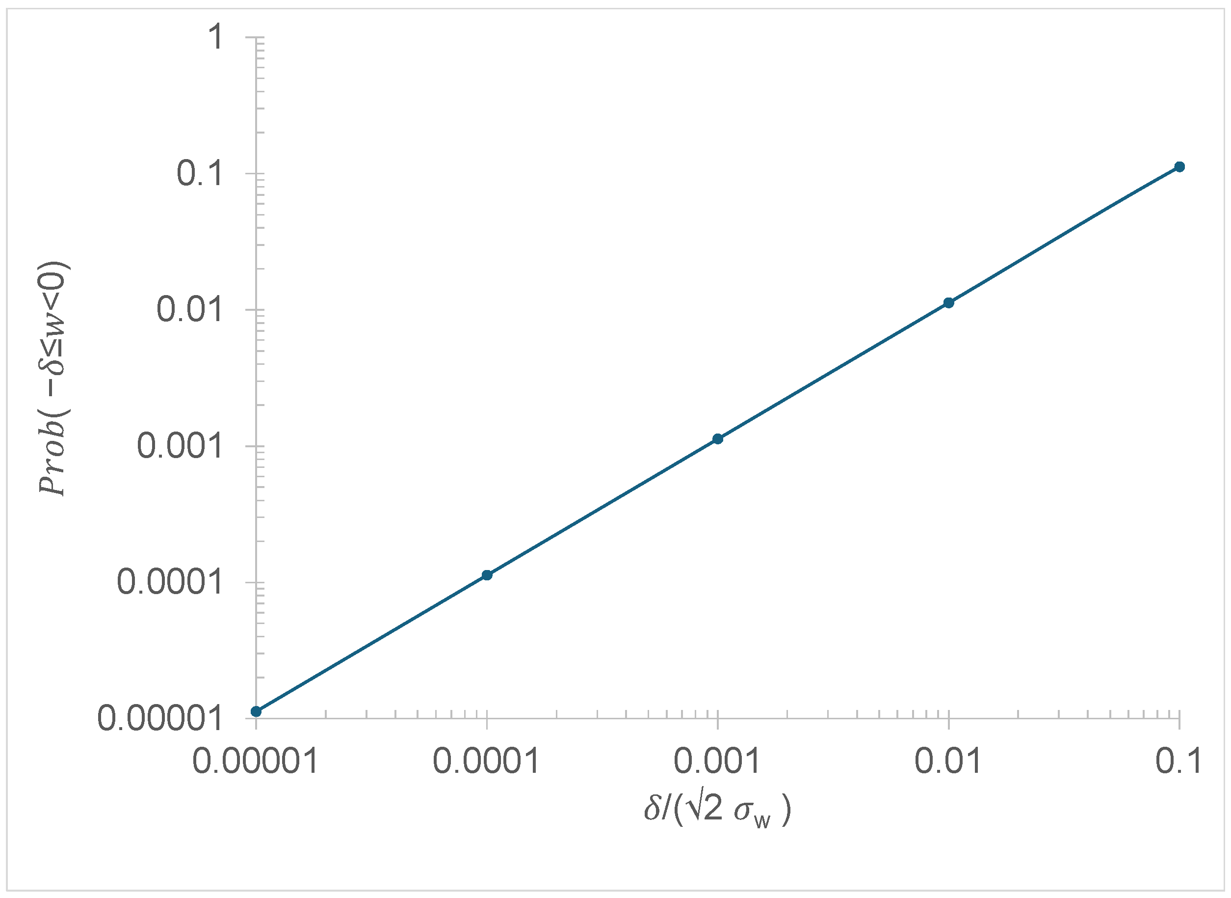
where erf x is the error function [30]. It should be noted that P r o b   0   <   w     δ   in (5) is the same as P r o b     δ     w   <   0 in the bLS modeling. Figure 2 shows that the probability of having w 2 σ w     10     3 is about 10−3, i.e., if the negative vertical velocities are sampled 1000 times in the bLS modeling, the likelihood is high of having one velocity with a magnitude no greater than 2 σ w   ×   10     3 .
The above analysis shows that for Gaussian turbulence there is a high probability of having a negative vertical velocity of a very small magnitude in the bLS modeling. More specifically, if the negative velocities are sampled 10n times, it is very likely to have one velocity whose magnitude is about 10–n m/s. The implication for bLS modeling is that the estimated ratio (C/Q)sim can be affected by the presence of some very small vertical velocities that tracer particles may possess when touching down on the emission source. For non-Gaussian turbulence it is expected that the same problem exists, although we cannot present a rigorous proof here.
We now specifically examine the FWY concentration estimator. It should be noted that the following analysis is valid for both Gaussian and non-Gaussian turbulence. Assume in the bLS model calculation that there are M ( M N ) back-flying tracer particles touching the source area. Let us further assume that among these M particles there is one particle having a very small magnitude of vertical velocity, w0slow, and we refer to this particle as a slow-touchdown particle. If we separate the contributions from the slow-touchdown particle (whose touchdown velocity is w0slow) and remaining particles, (2) can be written as
C Q s i m = 1 N i = 1 M 2 w 0 i = 1 N i = 1 M 1 2 w 0 i + 1 N 2 w 0 s l o w = 2 ( M 1 ) N 1 w 0 m e a n ¯ + 2 N w 0 s l o w ,
where 1 / w 0 m e a n ¯ is the mean of the absolute value of the receptacle of touchdown velocities, excluding the slow-touchdown particle. Rearranging the right-hand side of (6), we have
C Q s i m = 2 ( M 1 ) N 1 w 0 m e a n ¯ 1 + 1 w 0 s l o w M 1 1 w 0 m e a n ¯ .
To obtain a stable estimate for C / Q s i m , M needs to be far greater than unity, so (7) can be approximated as
C Q s i m 2 M N 1 w 0 m e a n ¯ 1 + 1 w 0 s l o w M 1 w 0 m e a n ¯ .
on the condition that M 1 . Denote f = 1 + 1 w 0 s l o w M 1 w 0 m e a n ¯   , it is apparent that with just one slow-touchdown particle C / Q s i m will be f times as high as that in the situation without the slow-touchdown particle. For the convenience of discussion, a positive constant, α, is introduced. It is obvious that when w 0 s l o w α / M 1 / w 0 m e a n ¯ , f 1 + 1 / α , i.e., the ratio, C / Q s i m , is at least 1 + 1 / α times as high as what is obtained without the presence of the slow-touchdown particle. Limiting the minimum allowable vertical velocity is not the solution to this problem since, as shown in Figure 1, setting a minimum allowable velocity in the modeling may artificially change the final outcome of the estimate for C / Q s i m .
It is worthwhile to note that for any given M and N, there may be multiple slow-touchdown particles. Denoting the number of slow-touchdown particles as m ( m M ), then to result in the same level of impact on C / Q s i m , the magnitude of the velocity of slow-touchdown particles needs to satisfy 1 / 1 / w 0 s l o w ¯ α m / M 1 / w 0 m e a n ¯ , a condition that is easier to meet. Obviously, the existence of multiple slow-touchdown particles will make the situation even worse. In any event, the modeled ratio C / Q s i m can be significantly affected by the presence or absence of slow-touchdown particles.
The above analysis shows that the FWY estimator may be significantly affected by the existence of slow-touchdown particles and there is no reason to expect the slow-touchdown particles to not be present.

2.3. An Alternative Concentration Estimator

In the following we propose an alternative concentration estimator.
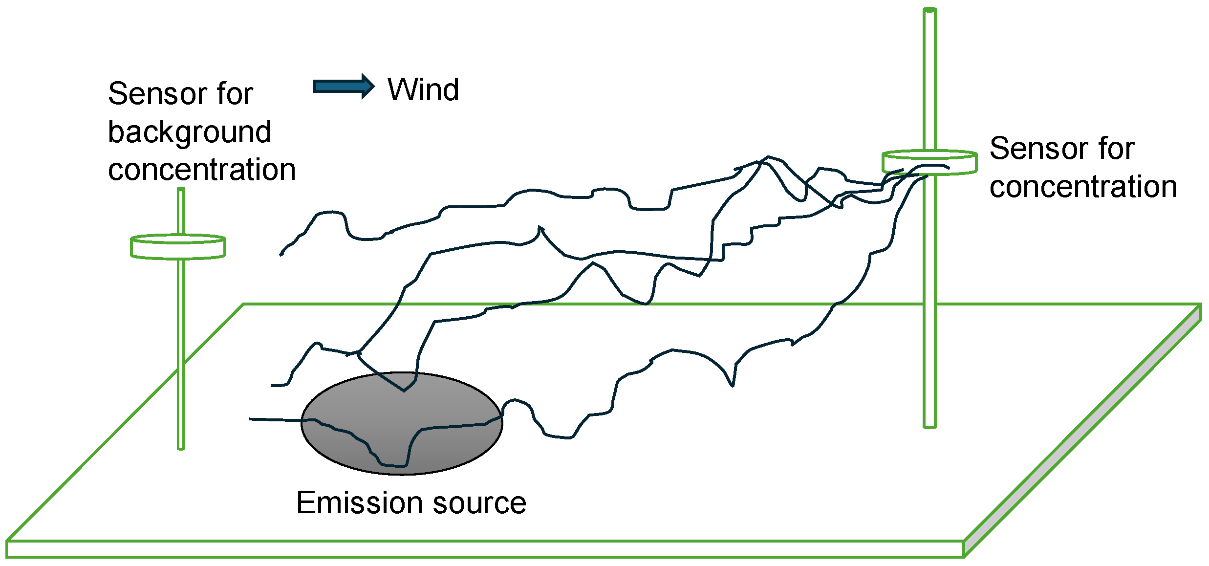
Consider the field experiment setup schematically shown in Figure 3. The concentration is measured by a sensor mounted on a mast that is located downwind of a ground-to-air emission source (i.e., in the plume emitted from the source). Near the source is a meteorological tower (not shown in the drawing) that has instruments to measure micrometeorological conditions needed to carry out the bLS simulation. Immediately upwind of the source the background concentration is measured by another sensor.
Release N particles from the concentration sensor and follow them backward with a bLS model. Assume M of these particles hit the emission source during the backward flights, and assume further that the kth particle hitting the emission source has a concentration of ck, then the concentration at the sensor is
C s i m = 1 N k = 1 M c k .
where Csim is the concentration obtained from the bLS model with the assumed emission rate, Qsim. Please note that the back-flying particles that do not hit the source will identically have a concentration of zero. c k can be related to the area of the source, S, and the emission rate from the entire area source, E (in g/s), by
0 S 1 M k = 1 M c k w p w d w = E .
It should be noted that (8) is applied to the “unresolved basal layer” (UBL), a very shallow layer in the vicinity of the ground. The UBL is so shallow in many cases that it is impractical to carry out any field measurement of flow and concentration statistics within the layer. The concept of UBL was introduced in [31] in the context of reflecting boundary conditions in LS modeling. The UBL may be comparable to the “roughness sublayer”, a layer encompassing and immediately above the roughness elements [32]. Because of the lack of knowledge regarding how ck varies within the UBL, to make progress we average (8) across the UBL 0 h U B L 0 S 1 M k = 1 M c k w p w d w d z = 0 h U B L E   d z . If we divide both sides by hUBL, the depth of the UBL, and denote the UBL-averaged quantities by angle brackets, we have S c 0 w p ( w ) d w = E , where c = 1 M k = 1 M c k . Since the top of the UBL is the same as, or close to, the bottom of the “outer layer” where empirical data exist for vertical turbulent velocities, it is helpful to relate w p ( w ) to its counterpart at the bottom of the “outer layer”, which is normally the lowest part of the atmospheric surface layer. Based on direct numerical simulation (DNS) studies [33,34,35] the standard deviation of vertical velocities increases approximately linearly from zero to the level at the top of the UBL, so it is reasonable to take
w p ( w ) = 1 2 w p h U B L
for positive velocities. For a vertically extensive UBL such as a canopy layer where field measurement can be performed, the above equation also approximately holds true [36,37].
If we write w ¯ = 0 w p ( w ) h U B L d w , and denote E / S = Q s i m (in g·m−2·s−1) we have
c = 2 Q s i m w ¯ .
Since c = 1 M k = 1 M c k and from (9) C s i m = 1 N k = 1 M c k , we have
C s i m = M N c .
Combine (11) and (12), and we obtain
C Q s i m = 2 M N w ¯ .
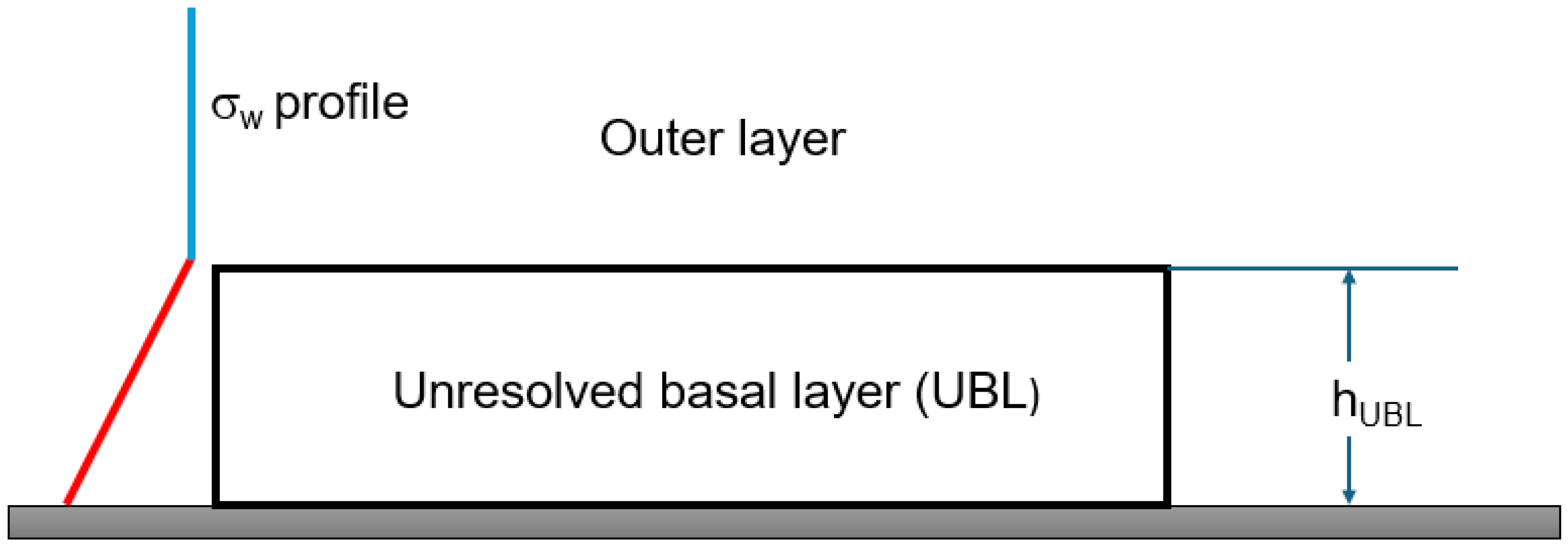
It should be noted that in the real space the counterpart of the touchdown velocity in bLS is actually the upward velocity w . It is also worth noting that w ¯ represents the mean upward flux of velocity (defined as 0 w p w d w ) .   Figure 4 presents a schematic drawing that facilitates the derivation of (12). Also, w ¯ needs to be evaluated at the top of the UBL, which in this work is treated as the bottom of the “outer layer” where the conventional atmospheric boundary layer scaling holds true.
Equation (13) resembles (2) very closely but there exists a fundamental difference between them: (2) contains the ensemble average of 1/w, while in (13) it is related to the ensemble average over w itself (instead of the reciprocal of w), which is well defined.
w ¯ can be related to conventional turbulence statistics. In LS modeling in the atmospheric boundary layer, the distribution of vertical velocity is often assumed to be Gaussian [3]. For Gaussian turbulence,
w ¯ = 0 w p w d w = 0 w 1 2 π σ w e w 2 2 σ w 2 d w = σ w 2 π .
In the convective boundary layer, it has been recognized that Gaussian distribution is not a good approximation and the distribution for vertical velocity can be approximated to be bi-Gaussian [38,39,40], i.e.,
p w = A p A + B p B = A 2 π σ A e w w A 2 2 σ A 2 + B 2 π σ B e w + w B 2 2 σ B 2 .
The basis for the bi-Gaussian distribution is that in the convective boundary layer there exist updrafts and compensating downdrafts. Within updrafts and downdrafts, the distributions of vertical velocities p A and p B can be considered to be Gaussian, respectively [38]. In (15) w A   a n d   σ A are the mean and standard deviation of vertical velocity in the updrafts, and w B   a n d   σ B are their counterparts in the downdrafts. A and B are the fractions of the horizonal areas covered by updrafts and downdrafts, respectively. From (15) it can be shown that
w ¯ = 0 w p w d w = 0 w A 2 π σ A e w w A 2 2 σ A 2 + B 2 π σ B e w + w B 2 2 σ B 2 d w   .
After several steps of mathematical manipulation and by taking σ A = w A and σ B = w B [38] we obtain
w ¯ = e 1 2 + π e r f 2 2 2 π A w A + B w B .
A, B, wA, and wB can be related to conventional turbulence statistics used in [38]
w B = w 3 ¯ 2 + 8 w 2 ¯ 3 w 3 ¯ 4 w 2 ¯ ,   w A = w 2 ¯ 2 w B ,     A = w B w A + w B ,   B = w A w A + w B ,
where w 2 ¯ is the second-order moment of the vertical velocity, commonly referred to as the variance of vertical velocity and denoted as σ w 2 , and w 3 ¯ is the third-order moment of the vertical velocity that quantifies how asymmetric the distribution of vertical velocity is.

3. Results

We tested the new concentration estimator in two types of turbulence: Gaussian turbulence and bi-Gaussian turbulence. For Gaussian turbulence, we used the model that was used in [11], and for bi-Gaussian turbulence, the model equations are presented in [28]. The applicable LS model equations are shown in Appendix A.
In the numerical simulation, a rectangular area source was placed at ground level. The source was 30 m long and 10 m wide. The four vertices were located at (–30 m, –5 m), (–30 m, 5 m), (0 m, 5 m), and (0 m, –5 m). Concentration sensors were placed at 1 m, 2 m, 3 m, 4 m, and 5 m heights and at three sampling distances: 0, 25, 50 m. N = 250,000 particles were released from each sensor and traced backward beyond the source area. In the simulation, the wind direction was assigned to be parallel to the longer side of the rectangle.
(C/Q)sim was calculated with particle trajectories generated by appropriate bLS models. For Gaussian turbulence, we studied two cases: (1) unstable atmospheric surface layer with friction velocity u* = 0.2 m/s and Monin–Obukhov length L = –15 m; and (2) neutral atmospheric surface layer with u* = 0.5 m/s. For bi-Gaussian turbulence, the following two cases were studied: (1) convective atmospheric boundary layer with convective velocity scale w* = 1.1 m/s, depth of mixed layer Zi = 1000 m, and u* = 0.2 m/s; and (2) convective boundary layer with w* = 2.0 m/s, Zi = 1000 m, and u* = 0.2 m/s. In all these cases, the surface roughness length, z0, was set to 0.01 m. For each case, both the FWY and the present concentration estimators were used to calculate (C/Q)sim from the same set of trajectories generated by the bLS model for the four aforementioned cases; therefore, the difference in (C/Q)sim for each case is attributable solely to the difference between the FWY estimator and Equation (13).
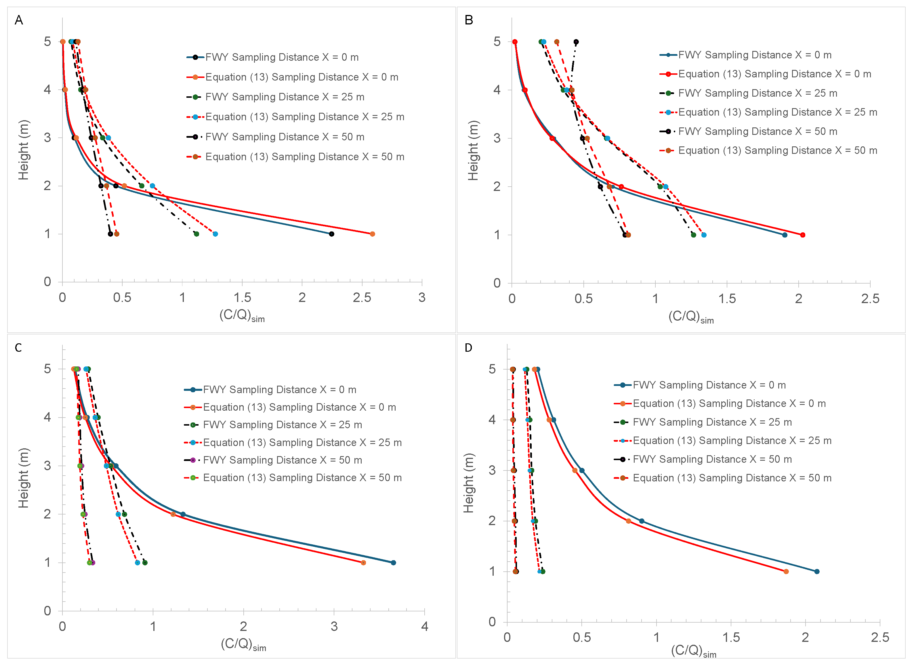
Figure 5 shows that for all these four cases and at most of the sampling locations, good agreement is achieved for the modeling results of (C/Q)sim obtained with FWY estimator and Equation (13). The only obvious exception is the case of the neutral atmospheric surface layer at just one sampling distance and one sensor height: in Figure 5B at the (50 m, 5 m) sensor, the (C/Q)sim calculated with the FWY estimator is higher than that at 4 m height (and the same distance). Such an abnormality is physically impossible. It is unlikely that the abnormality is attributable to the scantness of touchdowns—for this particular case the number of touchdowns was over 10,000.
We scanned the list of touchdown velocities. We found that the smallest velocity was 5.93 × 10     5 m/s. Clearly, it was this stagnant particle that caused the problem for the FWY estimator.
The abnormal (C/Q)sim at (50 m, 5 m) in case B demonstrates that sometimes slow-touchdown particles can indeed cause problems for the FWY estimator, although in most cases the FWY estimator works well. On the other hand, the good performance of FWY in most cases of our sensitivity test explains why in many studies the potential inaccuracy in the FWY estimator has not seemed to cause serious problems. One of the possible reasons why the deficiency has slipped through many studies is that the irregularity was buried in the statistical noise, especially when the number of tracer particles was not adequately large. Another reason is that the stagnant particles did not have the chance to hit the source area.

4. Discussion and Conclusions

We have shown that the FWY concentration estimator for bLS modeling of ground-to-air emissions can potentially be in error when the vertical movement of one or more tracer particles is extremely slow, or in other words, there may exist some slow-touchdown particles that cause significant error in the estimation of concentrations. We have also shown that this type of slow-touchdown particles cannot be eliminated by artificially imposing a minimum allowable vertical velocity. Clearly, for a prescribed number of tracer particles there does not exist a means to control how many particles would end up with touchdown vertical velocities in a pre-determined range, although the probability is known. As such, for any given modeling run, the number of particles with very small touchdown velocity is actually random; as shown in the previous section, the estimated ratio (C/Q)sim is strongly affected by the number of these vertically slow-moving particles. Since the latter is random (unless the number of tracer particles released is impractically large to make the fraction of these slow-moving particles invariant in each modeling run), the uncertainty in the estimated (C/Q)sim can be substantial. As a result, this means that, whether the purpose of bLS modeling is to estimate concentrations from the known emission rate Q or to estimate the emission rate from measured concentrations, the FWY estimator may result in inaccurate results. For the purpose of estimating concentrations from known emission rates, downwind concentrations can be significantly overestimated. On the other hand, if the purpose is to estimate emission rates from measured concentrations, the emission rates can be underestimated to a large extent. The new estimator is free of this type of difficulty so it is expected to give reliable results. In short, the fundamental difference between the two concentration estimators is that the vertically slow-moving particles can cause trouble for the FWY estimator but not for the new estimator.
Another difference between the FWY estimator and the new estimator is that the former is strictly valid under the stationary condition, while the latter is not subject to this restriction. Although it is difficult to quantify how much error would be introduced when the stationary condition is not met, the FWY estimator is not recommended for usage in long-range applications since during the tracer particles’ long flights the meteorological conditions are likely to change with time. By contrast, the new estimator can be used in long-range applications since it is obtained without invoking the stationary condition.
It should be noted that the comparison between the FWY estimator and the new estimator has been carried out with simple source configurations and ideal flow conditions. Since the effects of complex source configuration and non-ideal flow conditions only affect the trajectories of tracer particles, it is expected that the same conclusions about the concentration estimators will be reached if the test cases include these complicating factors.
Since the new concentration estimator often (but not always) gives about the same result as the FWY estimator, it is worthwhile to use both concentration estimators when utilizing the bLS modeling technique to calculate the ratio (C/Q)sim. If the values of (C/Q)sim obtained from both estimators are about the same, it is an indication that the slow-moving particles do not cause a significant problem for the FWY estimator. On the other hand, if (C/Q)sim calculated with FWY is noticeably different from that obtained with the new estimator, there is a need to examine if there are any particles that are touching the source area with extremely slow vertical velocities. A rule of thumb to decide whether a vertical velocity is extremely slow is that the velocity is of the order of σ w / M , where M is the total number of times that tracer particles hit the source. Since removing the vertically slow-moving particles is not scientifically well based, the result obtained with the new estimator is preferrable.

Author Contributions

Conceptualization, S.D.; Methodology, S.D. and C.S.; Software, B.W. and S.D.; Validation, B.W. and X.T.; Formal analysis, B.W., C.S., S.D. and X.T.; Investigation, B.W., C.S., W.W., X.T. and S.D.; Resources, C.S. and W.W.; Data curation, B.W.; Writing—original draft, W.W. and S.D.; Supervision, W.W.; Project administration, C.S. and W.W. All authors have read and agreed to the published version of the manuscript.

Funding

This research was funded by the National Research Program for Key Issues in Air Pollution Control, China, under project number DQGG2021101.

Data Availability Statement

The data presented in this study are available on request from the corresponding authors.

Acknowledgments

The authors are indebted to all four reviewers for their constructive reviews and helpful suggestions to improve the manuscript.

Conflicts of Interest

Author Biao Wang was employed by the company Taizhou Environmental Science Design and Research Institute Co., Ltd. The remaining authors declare that the research was conducted in the absence of any commercial or financial relationships that could be construed as a potential conflict of interest.

Nomenclature

SymbolDescription
Arelative frequency of occurrence of the updrafts (unitless)
Brelative frequency of occurrence of the downdrafts (unitless)
ckconcentration possessed by the kth particle hitting the emission source (in g/m3)
C s i m concentration obtained with the assumed emission rate, Qsim (in g m−3)
C0 Lagrangian velocity structure function constant (unitless)
Eemission rate from the entire area source (in g/s)
hUBLheight of the unresolved basal layer (in m)
LMonin–Obukhov length (in m)
Mnumber of particles that hit the source in backward flights (dimensionless)
Nnumber of particles released at each receptor in a run (dimensionless)
p(w)probability density function of vertical velocity (in m−1 s)
p A (w)probability density function of vertical velocity in updrafts (in m−1 s)
p B (w)probability density function of vertical velocity in downdrafts (in m−1 s)
Q emission rate from a ground-level source (in g m−2 s−1)
Q s i m assumed emission rate in Lagrangian modeling (in g m−2 s−1)
Sarea of the ground-level source (in m2)
u*friction velocity (in m s−1)
Uaverage wind speed (in m s−1)
w*convective velocity scale (in m s−1)
w A the mean vertical velocity in updrafts (in m s−1)
w B the negative mean vertical velocity in downdrafts (in m s−1)
w 2 ¯ the variance of vertical velocity (=   σ w 2 ) (in m2 s−2)
w 3 ¯ the third-order moment of vertical velocity (in m3 s−3)
w0touchdown velocity of tracer particle on the source area (in m s−1)
w ¯ defined as 0 w p ( w ) d w (in m s−1)
Zidepth of mixed layer under convective conditions (in m)
σ A the standard deviation of vertical velocity in updrafts (in m s−1)
σ B the standard deviation of vertical velocity in downdrafts (in m s−1)
σ u the standard deviation of streamwise turbulent velocity in downdrafts (in m s−1)
σ v the standard deviation of lateral turbulent velocity in downdrafts (in m s−1)
σ w the standard deviation of vertical turbulent velocity in downdrafts (in m s−1)
εthe average dissipation rate of turbulent kinetic energy (in m2 s−3)

Appendix A. Equations of Lagrangian Stochastic Models

Two sets of LS model equations were used in the numerical simulation. These sets of equations have been published elsewhere, but for the purpose of easier reference for the reader, they are listed as follows.
The general form of first-order LS models is the three-dimensional Langevin equation [3]
            d u = a u d t + C 0 ε 1 2 d ξ u ,               d x = u d t , d v = a v d t + C 0 ε 1 2 d ξ v ,               d y = v d t ,   d w = a w d t + C 0 ε 1 / 2 d ξ w ,             d z = w d t
where u, v, and w are the velocities of the tracer particle located at (x, y, z) in the streamwise, lateral, and vertical directions; au, au, and aw are the deterministic acceleration of the tracer particle in the streamwise, lateral, and vertical directions; ε is the averaged dissipation rate of turbulent kinetic energy (TKE); C0 is the Lagrangian velocity structure function constant and takes the value of 3.0 [41] in the present study; dξu, dξv, and dξw are independent Gaussian random numbers with mean 0 and variance dt. Ordinarily for studies of the atmospheric surface layer, the x-axis of the Cartesian coordinates is in the direction of average wind, so the average u is not zero and here we denote the average wind speed as U.
Flesch et al. [11] presented a three-dimensional model for Gaussian turbulence. All correlations between components of fluctuating velocities were ignored except the correlation between u and w , and only the vertical variation of σ w 2 is accounted for. Under these conditions and further taking the background turbulence as stationary, the LS model equations can be written as
a u = 1 2 σ u 2 σ w 2 u * 4 C 0 ε σ w 2 u U + u * 2 w + w U z ,
a v = 1 2 C 0 ε v σ v 2 ,
a w = 1 2 σ u 2 σ w 2 u * 4 C 0 ε u * 2 u U + σ u 2 w + 1 2 σ w 2 z + 1 2 σ u 2 σ w 2 u * 4 u * 2 σ w 2 z u U w + σ u 2 σ w 2 z w 2 .
All turbulence statistics needed are shown in [11].
For non-Gaussian turbulence, we used the Luhar and Sawford model [28]. In the model, correlations between all velocity components are neglected. Under the conditions of horizontal homogeneity and of vanishing spatial variation of σ u 2 , the equation for aw is reduced to that of [39], so the model equations can be written as
a u = C 0 ε 2 σ u 2 ( u U ) + w U z ,
  a w = C 0 ε 2 p w Q w + φ w p w ,
where
  Q w = A ( w w A ) σ A 2 p A + B ( w + w B ) σ B 2 p B ,
φ w = 1 2 A w A z + w A A z e r f w w A 2 w A + w A A w A z w 2 w A 2 + 1 + w A A z p A + 1 2 B w B z + w B B z e r f w + w B 2 w B + w B B w B z w 2 w B 2 + 1 + w B B z p B ,
  p ( x , y , z ) w , x , z = A p A + B p B ,
p A w , x , z = A 2 π σ A e x p w w A 2 2 σ A 2 ,
    p B w , x , z = B 2 π σ B e x p w + w B 2 2 σ B 2 ,
  w B = w 3 ¯ 2 + 8 w 2 ¯ 3 w 3 ¯ 4 w 2 ¯ ,  
w A = w 2 ¯ 2 w B ,  
A = w B w A + w B ,  
B = w A w A + w B   .  
In the above equations, subscripts A and B stand for updrafts and downdrafts in the convective boundary layer, respectively. A and B are the relative frequencies of occurrence of updrafts and downdrafts, respectively. w A   a n d   σ A are the mean vertical velocity and the standard deviation in the updrafts, and w B   a n d   σ B are their counterparts in the downdrafts.
The equation for the lateral acceleration is
a v = C 0 ε 2 σ v 2 v .
Turbulence statistics needed to carry out model calculations in the modeling were specified as follows. w 2 ¯ and w 3 ¯ were the same as what were used in [28].
σ u = 2.5 u * 2 + 0.35 w * 2 1 / 2
and
σ v = 2.0 u * 2 + 0.35 w * 2 1 / 2
were adopted from Flesch et al. [12], where w* is the scale of convective velocity. The dissipation rate of TKE was taken as
ε = e z / Z i   4 σ w 3 3 z 1 6 z / L 1 / 4 ,
which was taken from [1] and modified with a factor to be applicable to the entire convectively boundary layer.

References

  1. Wilson, J.D.; Thurtell, G.W.; Kidd, G.E. Numerical simulation of particle trajectories in inhomogeneous turbulence, III: Comparison of predictions with experimental data for the atmospheric surface layer. Bound.-Layer Meteorol. 1981, 21, 443–463. [Google Scholar] [CrossRef]
  2. Legg, B.J.; Raupach, M.R. Markov-chain simulation of particle dispersion in inhomogeneous flows: The mean drift velocity induced by a gradient in Eulerian velocity variance. Bound.-Layer Meteorol. 1982, 24, 3–13. [Google Scholar] [CrossRef]
  3. Thomson, D.J. Criteria for the selection of stochastic models of particle trajectories in turbulent flows. J. Fluid Mech. 1987, 180, 529–556. [Google Scholar] [CrossRef]
  4. Pope, S.B. Consistency conditions for random-walk models of turbulent dispersion. Phys. Fluids 1987, 30, 2374–2379. [Google Scholar] [CrossRef]
  5. Wilson, J.D.; Sawford, B.L. Review of Lagrangian stochastic models for trajectories in the turbulent atmosphere. Bound.-Layer Meteorol. 1996, 78, 191–210. [Google Scholar] [CrossRef]
  6. Lin, J.; Brunner, D.; Gerbig, C.; Stohl, A.; Luhar, A.; Webley, P. (Eds.) Lagrangian Modeling of the Atmosphere; John Wiley & Sons: Hoboken, NJ, USA, 2013. [Google Scholar]
  7. Hurley, P.J.; Physick, W.L.; Luhar, A.K. TAPM: A practical approach to prognostic meteorological and air pollution modelling. Environ. Model. Softw. 2005, 20, 737–752. [Google Scholar] [CrossRef]
  8. Gariazzo, C.; Papaleo, V.; Pelliccioni, A.; Calori, G.; Radice, P.; Tinarelli, G. Application of a Lagrangian particle model to assess the impact of harbour, industrial and urban activities on air quality in the Taranto area, Italy. Atmos. Environ. 2007, 41, 6432–6444. [Google Scholar] [CrossRef]
  9. Yee, E. Theory for reconstruction of an unknown number of contaminant sources using probabilistic inference. Bound.-Layer Meteorol. 2008, 127, 359–394. [Google Scholar] [CrossRef]
  10. Stein, A.F.; Draxler, R.R.; Rolph, G.D.; Stunder, B.J.B.; Cohen, M.D.; Ngan, F. NOAA’s HYSPLIT atmospheric transport and dispersion modeling system. Bull. Am. Meteorol. Soc. 2015, 96, 2059–2077. [Google Scholar] [CrossRef]
  11. Flesch, T.K.; Wilson, J.D.; Harper, L.A.; Crenna, B.P.; Sharpe, R.R. Sharpe, Deducing Ground-to-Air Emissions from Observed Trace Gas Concentrations: A Field Trial. J. Appl. Meteorol. Climatol. 2004, 43, 487–502. [Google Scholar] [CrossRef]
  12. Flesch, T.; Wilson, J.; Harper, L.; Crenna, B. Estimating gas emission from a farm using an inverse-dispersion technique. Atmos. Environ. 2005, 39, 4863–4874. [Google Scholar] [CrossRef]
  13. Prajapati, P.; Santos, E.A. Comparing methane emissions estimated using a backward-Lagrangian stochastic model and the eddy covariance technique in a beef cattle feedlot. Agric. For. Meteorol. 2018, 256, 482–491. [Google Scholar] [CrossRef]
  14. Baldocchi, D.D.; Wilson, K.B. Modeling CO2 and water vapor exchange of a temperate broadleaved forest across hourly to decadal time scales. Ecol. Model. 2001, 142, 155–184. [Google Scholar] [CrossRef]
  15. Woodward, F.I.; Lomas, M.R. Vegetation dynamics–simulating responses to climatic change. Biol. Rev. 2004, 79, 643–670. [Google Scholar] [CrossRef]
  16. Wysocka-Czubaszek, A.; Czubaszek, R.; Roj-Rojewski, S.; Banaszuk, P. Methane and nitrous oxide emissions from agriculture on a regional scale. J. Ecol. Eng. 2018, 19, 206–217. [Google Scholar] [CrossRef]
  17. Mikkelsen, R. Ammonia emissions from agricultural operations: Fertilizer. Better Crops 2009, 93, 9–11. [Google Scholar]
  18. Flesch, T.K.; Wilson, J.D.; Yee, E. Backward-time Lagrangian stochastic dispersion models, and their application to estimate gaseous emissions. J. Appl. Meteorol. 1995, 34, 1320–1332. [Google Scholar] [CrossRef]
  19. Loubet, B.; Milford, C.; Sutton, M.A.; Cellier, P. Investigation of the interaction between sources and sinks of atmospheric ammonia in an upland landscape using a simplified dispersion-exchange model. J. Geophys. Res. Atmos. 2001, 106, 24183–24195. [Google Scholar] [CrossRef]
  20. McBain, M.; Desjardins, R. The evaluation of a backward Lagrangian stochastic (bLS) model to estimate greenhouse gas emissions from agricultural sources using a synthetic tracer source. Agric. For. Meteorol. 2005, 135, 61–72. [Google Scholar] [CrossRef]
  21. Denmead, O.T. Approaches to measuring fluxes of methane and nitrous oxide between landscapes and the atmosphere. Plant Soil 2008, 309, 5–24. [Google Scholar] [CrossRef]
  22. Ni, K.; Köster, J.R.; Seidel, A.; Pacholski, A. Field measurement of ammonia emissions after nitrogen fertilization—A comparison between micrometeorological and chamber methods. Eur. J. Agron. 2015, 71, 115–122. [Google Scholar] [CrossRef]
  23. Riva, C.; Orzi, V.; Carozzi, M.; Acutis, M.; Boccasile, G.; Lonati, S.; Tambone, F.; D’IMporzano, G.; Adani, F. Short-term experiments in using digestate products as substitutes for mineral (N) fertilizer: Agronomic performance, odours, and ammonia emission impacts. Sci. Total Environ. 2016, 547, 206–214. [Google Scholar] [CrossRef]
  24. Yang, W.; Zhu, A.; Zhang, J.; Zhang, X.; Che, W. Assessing the backward Lagrangian stochastic model for determining ammonia emissions using a synthetic source. Agric. For. Meteorol. 2016, 216, 13–19. [Google Scholar] [CrossRef]
  25. Lam, S.K.; Suter, H.; Davies, R.; Bai, M.; Mosier, A.R.; Sun, J.; Chen, D. Direct and indirect greenhouse gas emissions from two intensive vegetable farms applied with a nitrification inhibitor. Soil Biol. Biochem. 2018, 116, 48–51. [Google Scholar] [CrossRef]
  26. Shaw, J.T.; Allen, G.; Pitt, J.; Shah, A.; Wilde, S.; Stamford, L.; Fan, Z.; Ricketts, H.; Williams, P.I.; Bateson, P.; et al. Methane flux from flowback operations at a shale gas site. J. Air Waste Manag. Assoc. 2020, 70, 1324–1339. [Google Scholar] [CrossRef] [PubMed]
  27. Rodean, H.C. Stochastic Lagrangian Models of Turbulent Diffusion. Meteorol. Monogr. 1996, 26, 1–84. [Google Scholar] [CrossRef]
  28. Luhar, A.K.; Sawford, B.L. Lagrangian stochastic modeling of the coastal fumigation phenomenon. J. Appl. Meteorol. Climatol. 1995, 34, 2259–2277. [Google Scholar] [CrossRef]
  29. Wall, H.S. Analytic Theory of Continued Fractions; Chelsea Publishing Company: New York, NY, USA, 1948. [Google Scholar]
  30. Press, W.H.; Vetterling, W.T.; Teukolsky, S. Numerical Recipes: The Art of Scientific Computing, 3rd ed.; Cambridge University Press: New York, NY, USA, 2007; ISBN 978-0-521-88068-8. [Google Scholar]
  31. Wilson, J.D.; Flesch, T.K. Flow boundaries in random flight dispersion models: Enforcing the well-mixed condition. J. Appl. Meteorol. 1993, 32, 1695–1707. [Google Scholar] [CrossRef]
  32. Raupach, M.R.; Antonia, R.A.; Rajagopalan, S. Rough-Wall Turbulent Boundary Layers. Appl. Mech. Rev. 1991, 44, 1–25. [Google Scholar] [CrossRef]
  33. Bhaganagar, K.; Kim, J.; Coleman, G. Effect of roughness on wall-bounded turbulence. Flow Turbul. Combust. 2004, 72, 463–492. [Google Scholar] [CrossRef]
  34. Ismail, U.; Zaki, T.A.; Durbin, P.A. The effect of cube-roughened walls on the response of rough-to-smooth (RTS) turbulent channel flows. Int. J. Heat Fluid Flow 2018, 72, 174–185. [Google Scholar] [CrossRef]
  35. Ma, R.; Alamé, K.; Mahesh, K. Direct numerical simulation of turbulent channel flow over random rough surfaces. J. Fluid Mech. 2021, 908, A40. [Google Scholar] [CrossRef]
  36. Finnigan, J. Turbulence in plant canopies. Annu. Rev. Fluid Mech. 2000, 32, 519–571. [Google Scholar] [CrossRef]
  37. Nemitz, E.; Loubet, B.; Lehmann, B.E.; Cellier, P.; Neftel, A.; Jones, S.K.; Hensen, A.; Ihly, B.; Tarakanov, S.V.; Sutton, M.A. Turbulence characteristics in grassland canopies and implications for tracer transport. Biogeosciences 2009, 6, 1519–1537. [Google Scholar] [CrossRef]
  38. Baerentsen, J.H.; Berkowicz, R. Monte Carlo simulation of plume dispersion in the convective boundary layer. Atmos. Environ. 1984, 18, 701–712. [Google Scholar] [CrossRef]
  39. Luhar, A.K.; Britter, R.E. A random walk model for dispersion in inhomogeneous turbulence in a convective boundary layer. Atmos. Environ. 1989, 23, 1911–1924. [Google Scholar] [CrossRef]
  40. Du, S.; Wilson, J.D.; Yee, E. Probability density functions for velocity in the convective boundary layer, and implied trajectory models. Atmos. Environ. 1994, 28, 1211–1217. [Google Scholar] [CrossRef]
  41. Du, S. Universality of the Lagrangian velocity structure function constant (C0) across different kinds of turbulence. Bound.-Layer Meteorol. 1997, 83, 207–219. [Google Scholar] [CrossRef]
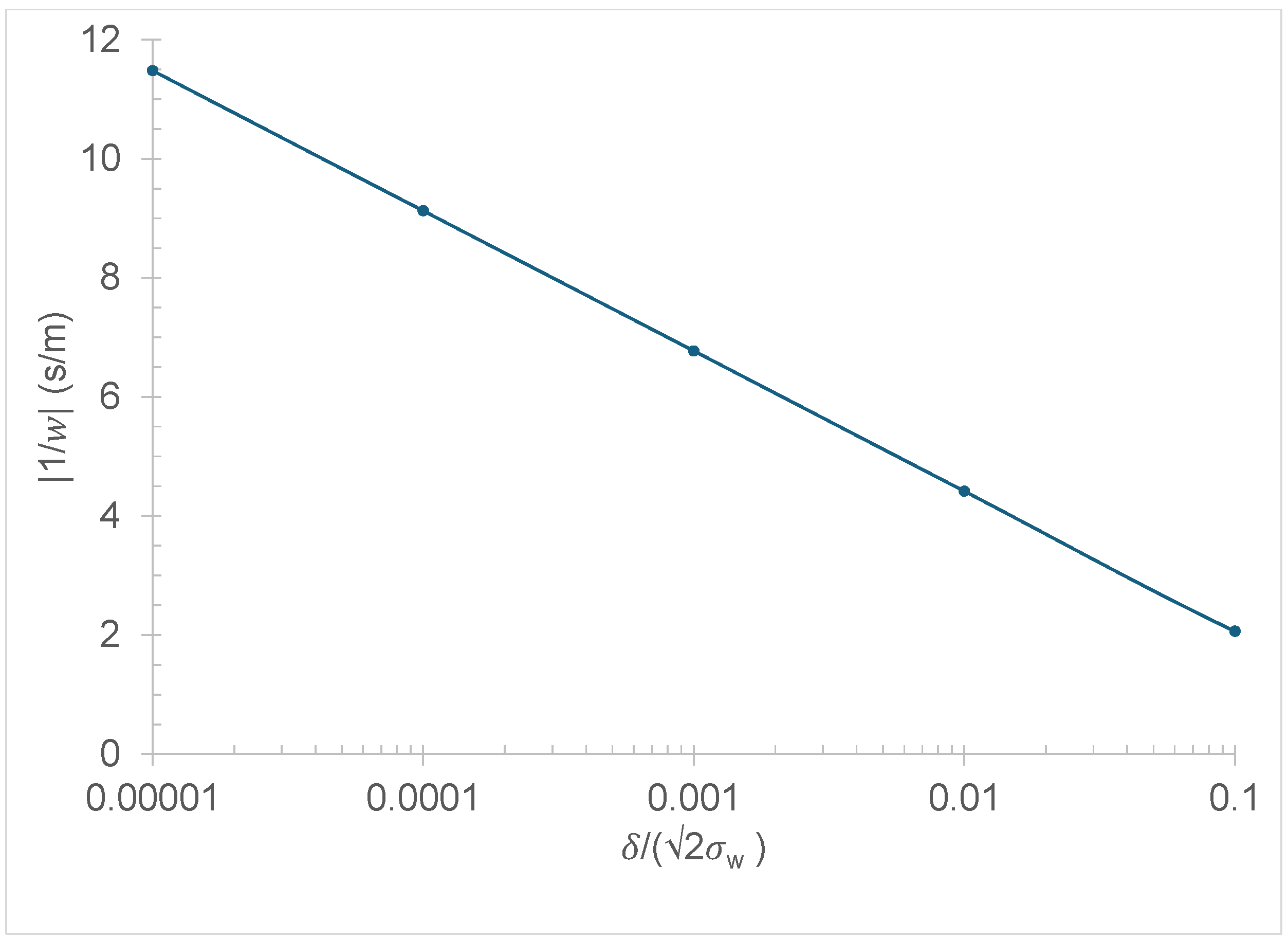
Figure 1. Ensemble average of 1 / w of source-touching particles in the bLS modeling for Gaussian turbulence. In the calculation, sw is set to be 0.39 m/s, a typical value in the atmospheric surface layer under near-neutral conditions.
Earth 06 00105 g001
Figure 2. The probability of the magnitude of the negative velocity in bLS modeling is no greater than certain levels.
Earth 06 00105 g002
Figure 3. A sketch showing the setup of a field experiment to estimate the emission rate with the bLS modeling.
Earth 06 00105 g003
Figure 4. A schematic sketch showing the UBL and the standard deviation of vertical velocity within it.
Earth 06 00105 g004
Figure 5. Comparison of (C/Q)sim obtained with the FWY estimator and a new estimator defined in Equation (13). The unit for (C/Q)sim is s/m, i.e., g m 3 / g m 2 · s . Four cases are shown: (A) Gaussian turbulence with u* = 0.2 m/s, L = –15 m; (B) Gaussian turbulence with u* = 0.5 m/s, neutral stratification; (C) bi-Gaussian turbulence with w* = 1.1 m/s, u* = 0.2 m/s, Zi = 1000 m; and (D) bi-Gaussian turbulence with w* = 2.0 m/s, u* = 0.2 m/s, Zi = 1000 m.
Earth 06 00105 g005
Disclaimer/Publisher’s Note: The statements, opinions and data contained in all publications are solely those of the individual author(s) and contributor(s) and not of MDPI and/or the editor(s). MDPI and/or the editor(s) disclaim responsibility for any injury to people or property resulting from any ideas, methods, instructions or products referred to in the content.