An Assessment of the Epicenter Location and Surroundings of the 24 January 2020 Sivrice Earthquake, SE Türkiye

Abstract

The Sivrice earthquake (Mw 6.8) occurred on 24 January 2020 along the East Anatolian Fault (EAF) zone of Türkiye, and epicentral information and focal mechanism solutions were published by two national and six international seismic stations. Here, we analyzed epicentral locations and the major fault trace using aerial photogrammetric images taken two days after, and synthetic aperture radar (SAR) interferometry. Although the focal mechanism solutions were similar, the epicenters were largely displaced. Several bright lineaments with a stair-like geometry were observed in aerial images of the Euphrates River channel along the fault trace. These lineaments, also called en echelon fractures in structural geology, are like right-lateral segments of a fault plane aligning the river channel, cut and offset by those similar in trend with the EAF and with alignments of a left lateral sense, as is the EAF motion sense. We interpret that the river local channel follows a right-lateral fault structure. The traces were lost a few days later, which proves the essentiality of remote sensing technologies for obtaining precise information in large regions. The time series analysis for one year period from Sentinel-1 SAR data also illustrated the displacements in the region sourced from the earthquake.

1. Introduction

According to the Disaster and Emergency Management Presidency (AFAD) of Türkiye, an earthquake of a magnitude of 6.8 occurred on 24 January 2020, at 20:55 Turkish time, with a duration of 20.4 s near the town Sivrice of Elazig Province, Türkiye. The event was located along the East Anatolian Fault (EAF), one of the major strike-slip fault zones of Türkiye. The earthquake was followed by multiple aftershocks, with the greatest magnitude being 5.0 Mw. The focal mechanism, epicentral location, rupture process, source mechanism, and tectonics were studied by different groups [1,2].

The Sivrice (Elazig) 24 January 2020 earthquake has been studied by a number of scholars for different aspects. Gunaydin et al. [3] provided the seismological characteristics of the earthquake and the damages caused by the shake. Isik et al. [4], Atmaca et al. [5], Yurdakul et al. [6], Bayrak et al. [7], Sayin et al. [8], Nemutlu et al. [9], and Caglar et al. [10] also analyzed the earthquake effects for geotechnical aspects including structural damages in terms of construction materials and crafts. Cetin et al. [11] assessed the site for geotechnical aspects, and reported on soil conditions, large constructions, rock fall, liquefaction, etc. Karakas et al. [12] compiled a co-seismic landslide inventory after the event and assessed the potential of stereo-aerial imagery and volumetric analysis for this purpose. Yalcin et al. [13] investigated the usability of citizen science methods for the rapid production of iso-intensity maps.

In addition, Konca et al. [14] analyzed surface rupture with Global Navigation Satellite Systems (GNSS) surveys and Sentinel-1 synthetic aperture radar (SAR) interferograms. The results indicated the partial rupturing of the Sivrice-Pütürge segment (45 km) with no significant surface slips. On the other hand, Bayik et al. [15] analyzed data from permanent GNSS stations and Sentinel-1 data to identify surface deformations sourced from the event. The interferometric SAR (InSAR) method was used for this purpose. The results showed that the magnitude may have been smaller (6.6), with a fault length of 37 km and depth of 17 km. The strike, dip, and rake values were measured as 242°, 80°, and 1°, respectively.

Here, we analyzed the major fault trace with the help of field studies, aerial photogrammetric images taken two days after the earthquake, and SAR interferometric data. The epicentral information of the event was published by two national and six international seismic stations, along with the focal mechanism solutions. Although the solutions are similar, showing a high-angle dipping segment of the fault zone, the distribution of the epicenters is largely displaced. Two of them are nevertheless compatible for explaining a north-dipping earthquake plane and one along a fault segment joining the East Anatolian Fault trace. After the radiometric enhancement of stereo-aerial images taken on 26 January 2020, several light-colored lineaments with a star-like geometry were observed on the Euphrates River channel along the fault trace. Similar observations were made by geologists working along the northern parts of the river, near the epicentral area of the earthquake immediately after the earthquake, and they explained this as gas bubbling along cracks along the river channel. In structural geology, these lineaments, also called en echelon fractures, are like right-lateral segments of a fault plane aligning the river channel, cut and offset by those similar in trend with the EAF and with alignments of a left lateral sense, as is the EAF motion sense. We interpret that the Euphrates River local channel follows a right-lateral fault structure. A few days later, a geologist who was there declared having seen no anomaly along the river. This observation is important in the sense that aerial photogrammetry may make a contribution with valuable information being obtain within few days following large earthquakes.

On the other hand, we analyzed regional displacements using Sentinel-1 InSAR to relate them with the epicenter locations. In addition, we applied a time series deformation analysis for a one-year period (6 months before and after the event), and analyzed the yearly deformation trends in the region. To our knowledge, this is the first study to analyze the epicenter locations and surroundings with the help of aerial photogrammetry, radar remote sensing, and time series analysis.

2. General Characteristics of the Earthquake

There have been 299 M ≥ 4.0 earthquakes, the largest being 6.8, since 1900 in Elazig region, and there are 40 historical records of earthquakes before 1900 (AFAD, 2020). The locations of the main earthquake and aftershocks published by AFAD for this earthquake with a depth of 8.06 km from the surface are given in Figure 1. The closest settlement to the earthquake is the Çevrimtaş village in the Sivrice district of Elazig Province, and the distance to the earthquake’s epicenter is approximately 800 m. The maximum acceleration recorded by AFAD was 0.293 g [12]. Several reconnaissance reports were published soon after the earthquake [16,17]. According to AFAD, the earthquake occurred in the Sivrice-Pütürge segment of the left-lateral strike-slip East Anatolian Fault (EAF) zone, with a rupture of approximately 50–55 km [18]. The earthquake caused 547 structures to be destroyed, 6247 buildings to be severely damaged, 962 buildings to be moderately damaged, 10,273 buildings to be slightly damaged, and 180 buildings to be demolished [19]. While the earthquake killed 41 people, it injured 1600 others.

According to Kürçer et al. [20], surface deformations have developed in an approximately 48 km long section between Hazar Lake and Pütürge. These surface deformations were observed as fault-related Riedel shear fractures, inter-strike tension cracks, and surface fractures. The lengths of these fractures, which continue in intermittent geometry, usually range from a few meters to several hundred meters. No significant lateral displacements were observed on the fractures [20]. Further information on the study region can be found in Karakas et al. [12] and the earthquake-related publications mentioned above.

3. Materials and Methods

Here, we utilized stereo-aerial stereo, Sentinel-1 Interferometric SAR (InSAR) data, and focal solutions of several seismic stations for our analyses. We also performed time series analysis for one year to characterize the surface changes in the region.

3.1. Aerial Photogrammetric Datasets

Detailed investigations were carried out into the region using stereo-aerial photographs taken before and after the earthquake (see Karakas et al. [12]; Gokceoglu et al. [17]). The post-earthquake images were taken on 26 January 2020 from an airplane at an altitude of 6000–7000 m above sea level by the General Directorate of Mapping (HGM), Türkiye, with a 20 cm spatial resolution. An UltraCam Eagle M3 wide-format metric camera with a sensor size of 26,460 × 17,004 pixels (PAN) was used for this purpose [21]. The sensor is able to acquire images in red, green, blue, and near-infrared (NIR) channels and with a dynamic range of 14 bits (16,384 gray values). It is possible to expect horizontal and vertical accuracies of 5–20 cm from the 3D points produced from these images. The area where the photos were taken is given in Figure 2. Pre-event aerial images were taken in 2017 over Malatya Province and in 2018 over Elazig province with a 30 cm resolution. These datasets were previously utilized for other purposes, such as the derivation of a co-seismic landslide inventory (Karakas et al. [12]) and landslide susceptibility assessment (Karakas et al. [22]). A very-high-resolution digital surface model (DEM) and orthophotos (coordinated photographs in the map projection) were also produced with Agisoft Metashape Professional software version 1.8.1. The resolution of the DEM and the orthophotos of a selected sub-area can be seen in Figure 3. The calibrated camera parameters and adjusted image positions and orientations (external orientation parameters) were also provided by the HGM.

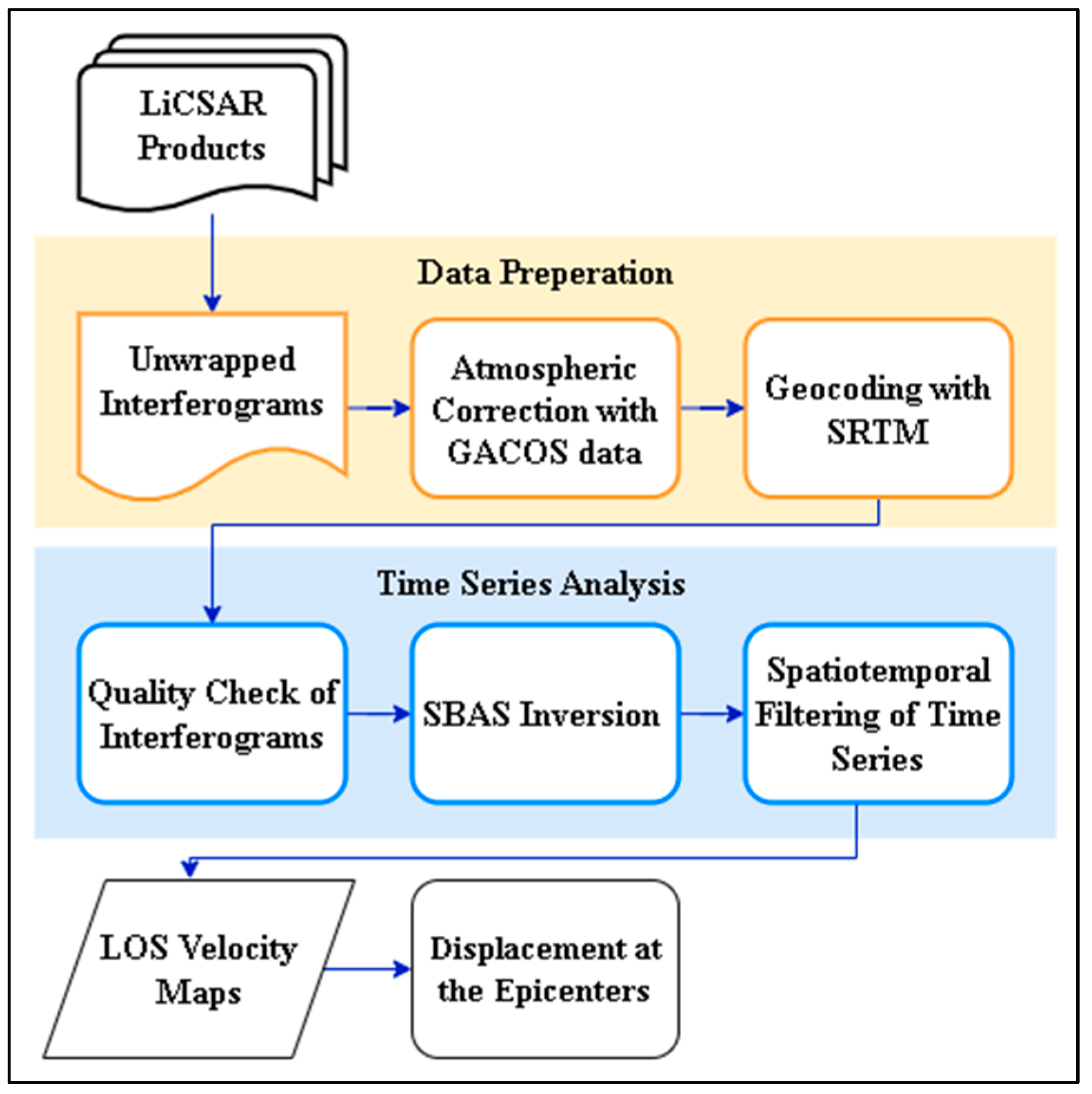
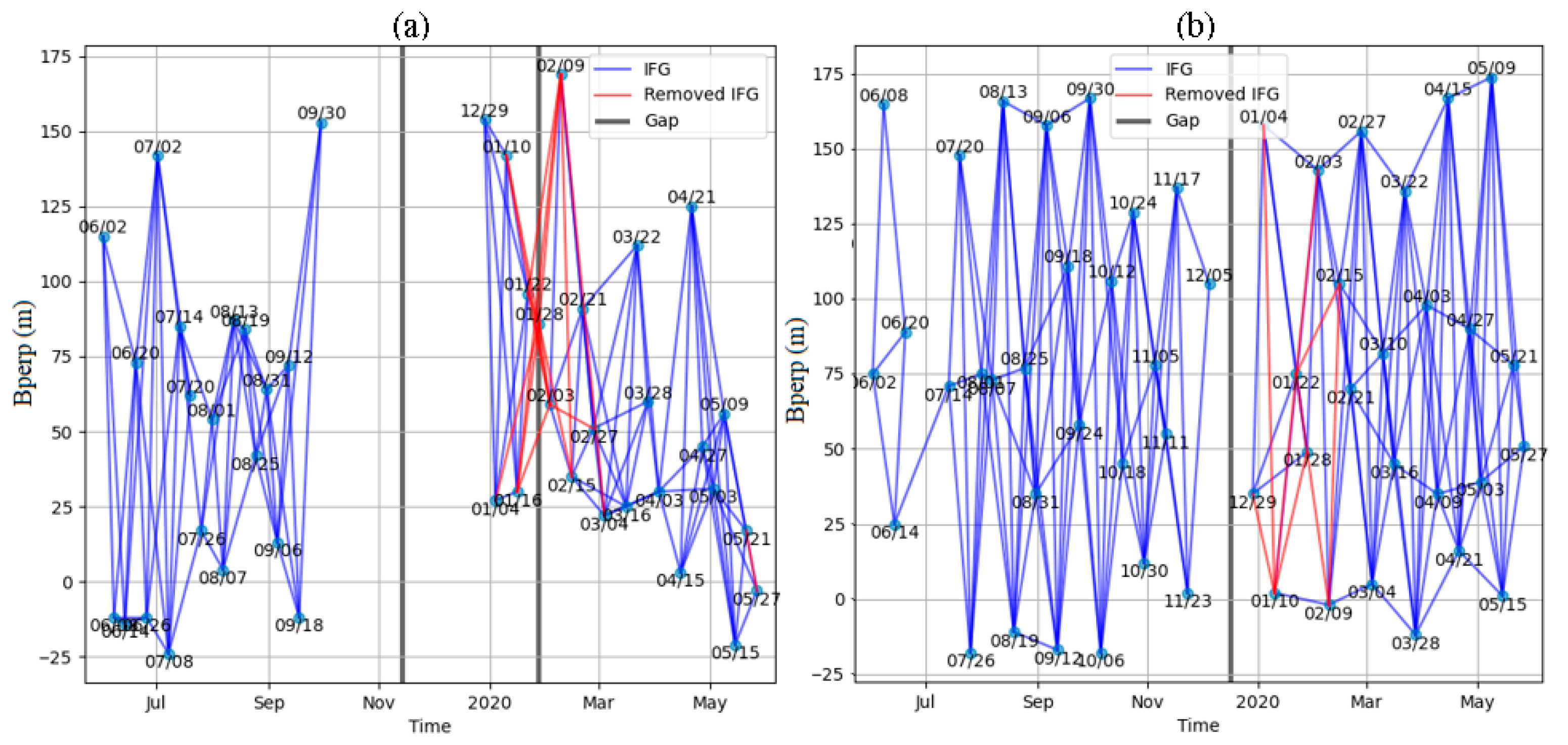
3.2. InSAR Datasets and Processing

Sentinel-1 is a collection of two identical near-polar orbiting satellites controlled by the European Space Agency (ESA) and belongs to the Copernicus program [23]. Sentinel-1A, which was launched on 3 April 2014, was followed by Sentinel-1B two years later, but Sentinel-1B could not continue its mission as of 23 December 2021. Therefore, the temporal resolution of Sentinel-1 data decreased from 6 days to 12 days. Sentinel-1 supplies product types at three levels (0, 1, and 2) of processing. These product types include single-look complex (SLC), ground range detected (GRD), ocean (OCN), and RAW with four sensor modes such as Stripmap (SM), interferometric wide swath (IW), extra-wide swath (EW), and wave (WV). While Level-1 SLC data include complex images with phase and amplitude, Level-1 GRD data include only systematically distributed multi-looked intensity.

In order to determine the changes on the surface with the InSAR method, two image pairs in total including Level-1 SLC products with the IW mode were used as shown in

Table 1. Properties of InSAR datasets.

Interfero gram	ID	Pass Direction	Mode	Date	Relative Orbit
i1	S1A_IW_SLC_....._F5DC	DSC	IW	16 January 2020	123
	S1A_IW_SLC_....._7D4F	DSC	IW	28 January 2020	123
i2	S1A_IW_SLC_....._1DB2	ASC	IW	22 January 2020	43
	S1A_IW_SLC_....._CB26	ASC	IW	28 January 2020	43

. The first pair denoted by i1 in Table 1 represents the descending (DSC) pass direction data dated 16 January 2020 and 28 January 2020, representing pre-event and post-event data, respectively. The second pair denoted by i2 represents the ascending (ASC) pass direction data dated 22 January 2020 and 28 January 2020, representing pre- and post-event data, respectively. These data were analyzed using SNAP software version 9.0.0, provided as an open-source software by ESA [24]. For each pair, data representations before and after the event were co-registered with enhanced spectral diversity (ESD). At this stage, Sentinel-1 precise orbit ephemeris was applied and then 1-arc-second Shuttle Radar Topography Mission elevation (SRTM HGT) was used together with the bilinear interpolation resampling method to eliminate the topographical phase effect. The ESD method was utilized to compute the displacements, and interferograms were produced [25]. Goldstein phase filtering and unwrapping were applied to relate topography [26]. The statistical-cost, network-flow algorithm for phase unwrapping (SNAPHU) package was used by applying the minimum cost flow (MCF) algorithm [27]. Finally, unwrapped phase of each dataset was converted into line-of-sight (LOS) displacement.

The deformations obtained with respect to the satellite line of sight (LOS) have been converted into absolute horizontal and vertical components on the Earth with the help of trigonometric equations and georeferencing methods. By using LOS displacement values produced in both (descending and ascending) orbits for each point, vertical and horizontal (East–West direction only) displacement magnitudes can be obtained using the geometric equations given in Equations (1) and (2) [28]:

$$d_e=\frac{D_{\mathit{d}}\mathit{cos}{\theta }_{\alpha }-D_{\alpha }\mathit{cos}{\theta }_d }{\mathit{sin}\left({\theta }_{\alpha }+{\theta }_d\right)}$$

(1)

$$d_z=\frac{D_{\mathit{d}}\mathit{sin}{\theta }_{\alpha }-D_{\alpha }\mathit{sin}{\theta }_d }{\mathit{sin}\left({\theta }_{\alpha }+{\theta }_d\right)}$$

(2)

where d_e and d_z represent the LOS displacement in the east–west and vertical directions, respectively. θ_α and θ_d are the look angles in both orbit modes and d is the displacement of a surface point, P.

For the time series analysis, LiCSAR products were used to apply the small baseline subset (SBAS) approach based on multi-temporal InSAR analysis [29]. The method was developed to facilitate the exploitation of SAR data for scientific and practical applications and proven to provide an accuracy of 7.5 mm based on comparisons with GNSS and leveling data [29]. LiCSAR, an InSAR processor developed by the Center for the Observation and Modelling of Earthquakes, Volcanoes, and Tectonics (COMET), is openly accessible through the COMET-LiCS interactive web portal [30]. This tool utilizes modified Copernicus Sentinel-1 data from the years 2015 to 2021, processed by COMET. Through this portal, wrapped and unwrapped interferograms as well as coherence maps are provided, resulting in a final product resolution of approximately 26.5 m. The products, derived from Sentinel-1 data, are systematically generated to monitor global tectonic and volcanic regions [31].

The SBAS methodology represents an advanced technique in multi-temporal InSAR analysis, obtaining LOS displacement velocity maps and time series analysis. In this context, the study employed LiCSBAS (version 1.5.11), an open-source Python3 package developed for conducting InSAR time series analysis. LiCSBAS comprises two main steps, data preparation and time series analysis, and uses a batch script with user-specified parameters [28,29]. Figure 4 illustrates the main steps and methodological workflow employed in this study. At the initial step of data preparation, LiCSAR products were downloaded, and the file formats were converted. The atmospheric phase screen (APS) is a crucial challenge in InSAR due to its main error source in interferograms. Many methods based on external meteorological data and phase have been developed to eliminate this error, which may cause displacement signals to be completely masked [32]. Here, the generic atmospheric correction model (GACOS), which is considered the most advanced external data-based method, was used for the tropospheric noise correction [33].

Followed by this step, pixels with an average coherence of ≤0.1 in the unwrapped data were masked to mitigate the effects of unwrapping errors, and all unwrapped interferograms and coherence data were clipped according to the specified area of interest. The unwrapped interferograms were then resampled and geocoded using the Shuttle Radar Topography Mission digital elevation model (SRTM DEM) with a 30 m resolution. In the second main step, low-quality interferograms were omitted from the dataset in accordance with coherence and unwrapped data coverage criteria (Figure 5). Finally, the updated unwrapped interferograms were inverted to generate maps of line-of-sight (LOS) displacement velocity and time series information.

In this study, LiCSAR data covering 1 year, from June 2019 to June 2020, were collected along both ascending (ID: 043A_05221_121313) and descending (ID: 123D_05095_141313) pass directions. The SBAS approach was applied as detailed in the study of Tavus et al. [34]. In total, 277 interferograms obtained from these two orbits were analyzed for this purpose and the results are presented in Section 4.3.

4. Results and Discussion

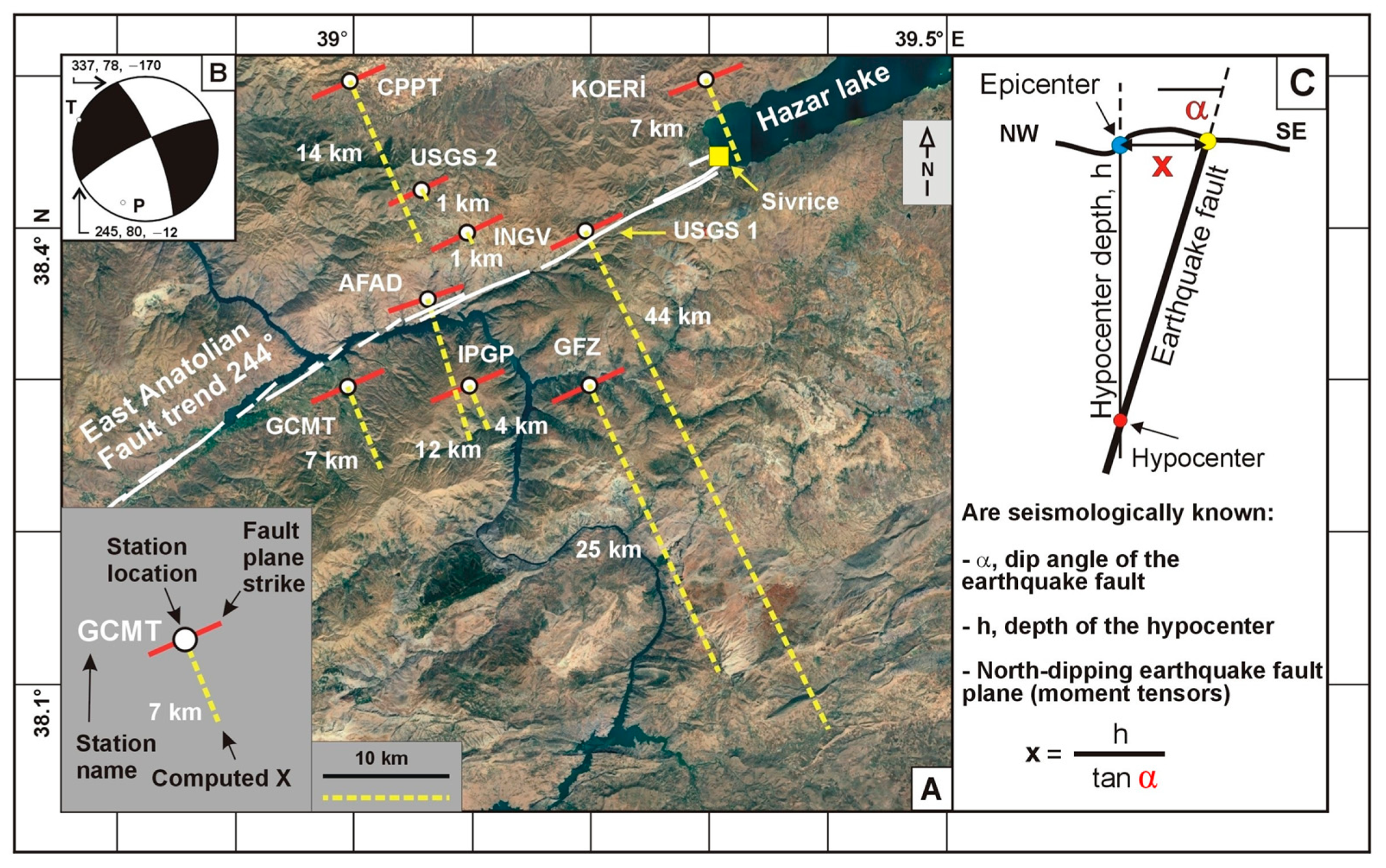
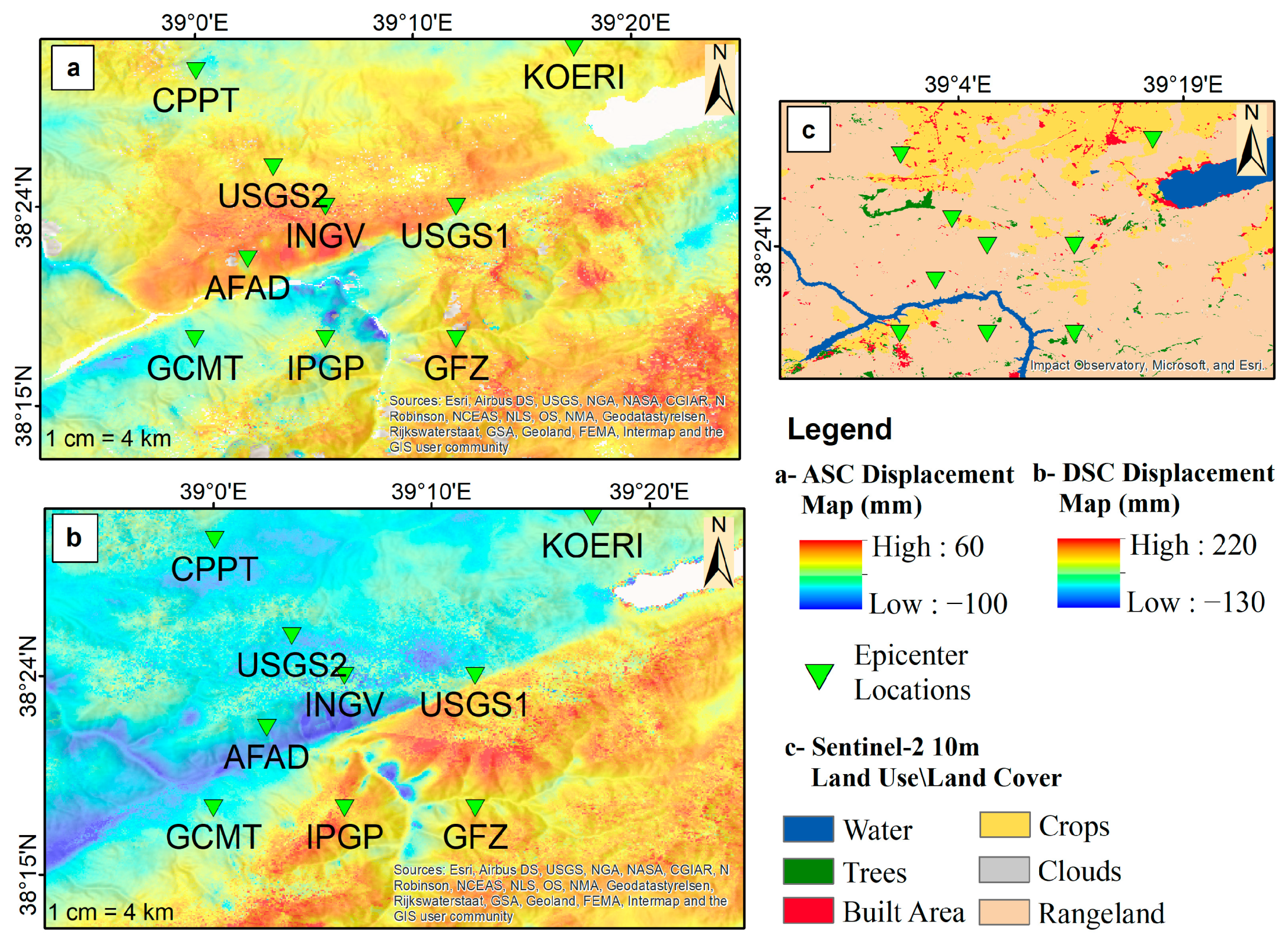
4.1. Epicentral Distribution of the Earthquake

The 24 January 2020 earthquake was studied by several seismic stations, giving the location of the event (Figure 6A) and some of them giving data related to the focal mechanism of the earthquake (Figure 6B). The stations included Global Centroid Moment Tensor Project (GCMT), Kandilli Observatory and Earthquake Research Institute (KOERI), French Polynesia Tsunami Warning Center (CPPT), GFZ German Research Center for Geosciences (GFZ), Istituto Nazionale di Geofisica e Vulcanologia (INGV), United States Geological Survey (USGS), Institut de Physique du Globe de Paris (IPGP), and Report of the Sivrice Earthquake of AFAD [18].

The focal mechanism solutions were very similar, displaying a high northwest dipping plane (

Table 2. Epicentral distribution and planes of focal solution data of the 24 January 2020 Sivrice earthquake. References: EMSC (2023) [35]; KOERI (2022) [36]; USGS (2022) [37]; AFAD (2020) [18].

Station	Lat. (°)	Lon. (°)	Depth (km)	Mag.	Strike 1 (°)	α, Dip1 (°)	Strike 2 (°)	α2, Dip2 (°)	X (km)	Ref.
GCMT	38.3	39.0	12	6.80	246	67	339	81	7	[35]
KOERI	38.52	39.29	10	6.70	339	85	248	87	7	[36]
CPPT	38.5	39.0	15	6.80	246	84	156	87	14	[35]
GFZ	38.3	39.2	20	6.80	338	68	245	81	25	[35]
INGV	38.4	39.1	11	6.80	244	58	338	84	1	[35]
USGS1	38.4	39.2	22	6.70	337	77	244	79	44	[35]
USGS2	38.431	39.061	10	6.70	337	78	245	80	1	[37]
IPGP	38.3	39.1	23	6.70	247	74	341	78	4	[35]
AFAD	38.35	39.06	8.06	6.80	248	76	158	89	12	[38]

) while the distribution of the epicenters was quite large. The latitude (Lat) and longitude (Lon) values given in Table 2 are in degrees. The depths are expressed in kilometers. Mag denotes the earthquake’s computed magnitude. Strike 1 and 2, α, Dip1 and α2, and Dip2 are the fault plane parameters and are given in degrees. X is the distance (in km) from the earthquake’s epicenter to the earthquake’s fault plane trace on the topographic surface (see Figure 6). Dark-colored strike cases in Table 2 show how different solutions are near to the 244° earthquake plane’s azimuth (measured from satellite images on Google Earth platform), while dip values are different in most cases. X is the minimum distance between the epicenter and the intersection of the earthquake plane with the topographic surface, calculated as in Figure 6C. We constructed a hypothetic NW–SE cross-section drawing (Figure 6C), orthogonal to the NW-dipping earthquake fault plane and the hypocenter depth; these two parameters were derived from seismic station web sites data (Table 2). This construction yielded the distance (x in Figure 6C) between the epicenter and the intersection of the earthquake’s fault plane with the topographic surface. Since field observations and interferometric data attest to the deformation along the major trace of the EAF, and not along another segment of the fault zone, we should find the intersection of the earthquake’s fault plane with the topographic surface on the major trace of the EAF.

Figure 6 shows that, first, epicenter locations (stations GCMT, IPGP, and GFZ) at the southeastern sector of the fault trace could not generate fault segments along the main trace of the East Anatolian Fault zone (EAFZ), and therefore cannot be considered reliable epicenter locations. The solution of AFAD is 12 km and does not generate a segment along the EAFZ main trace. This is also the case for the CPPT station, which generates a segment that is about 5 km NW of main earthquake’s fault trace, as is more or less the case for the station INGV. The KOERI station solution falls near Sivrice city and along the main trace of the EAFZ. We reached two solutions of the USGS, one being 44 km and another being 1 km. The earthquake’s epicenter fault trace distance of 1 km, constructed with data available from the NEIC Web page (USGS. [35]), also generates a segment that comes from the NW but far from the earthquake’s fault plane trace. The KOERI solution constructs a location that fits well with the earthquake’s fault trace, and this is the most unique solution among the several others.

In a digital era where several domains of human activity are equipped with artificial intelligence tools, it has become unacceptable to see such errors in the geophysical domain although their members are from the best users of computer-based works. We consider that (1) a reviewer may control the data to be published, as is conducted for NEIC-based solutions, and (2) an artificial intelligence contribution, possibly with a reviewer’s intervention, may be useful in preventing such errors.

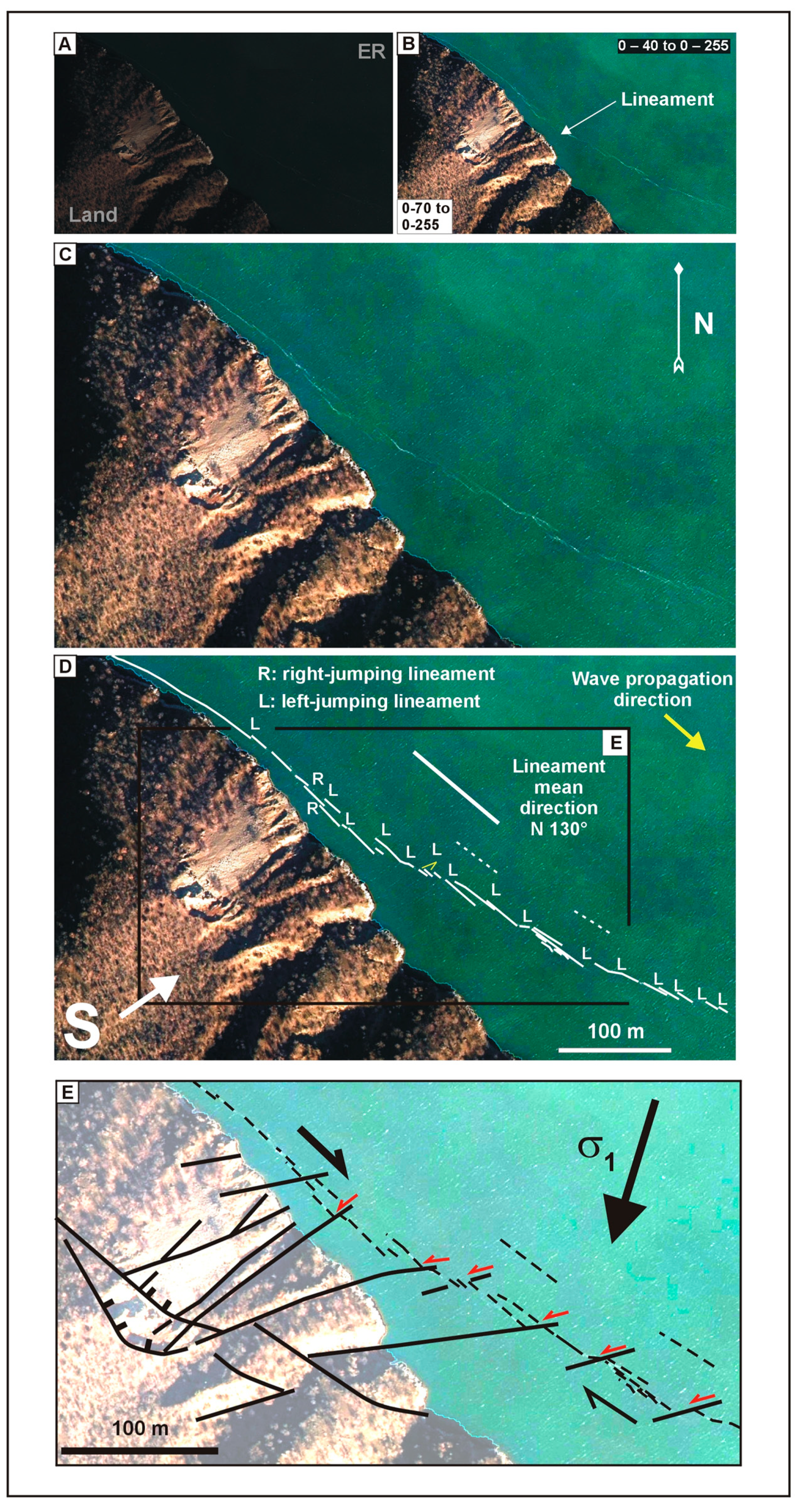
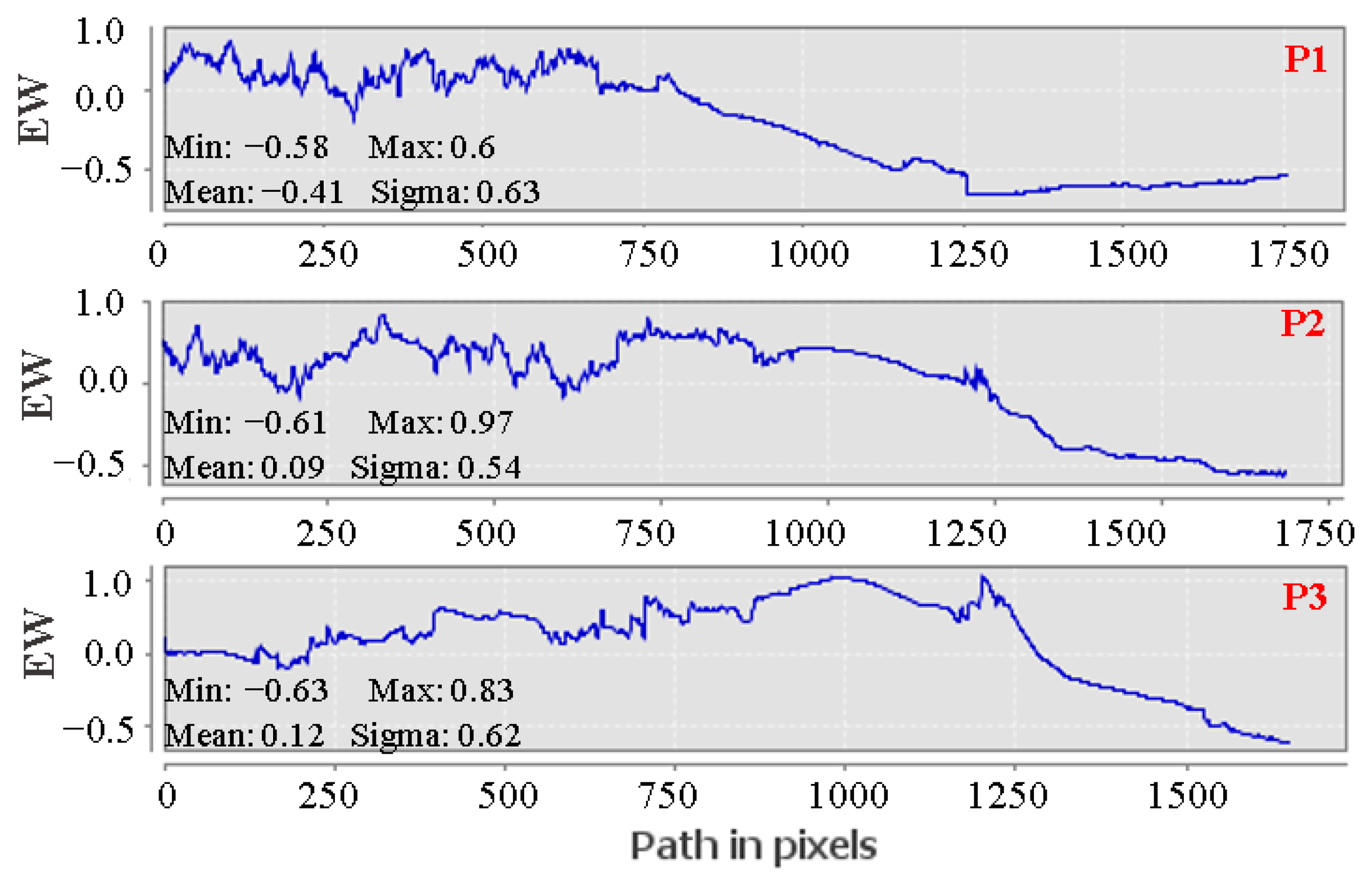
4.2. The Structural Motion along the Euphrates River Channel

Kürçer et al. [20] observed lineaments on the Euphrates River channel along the fault trace while working along the northern parts of the river, near the epicentral area of the earthquake (Figure 7). They explained this as gas bubbling along cracks along the river channel.

However, we have analyzed the very-high-resolution (20 cm) digital aerial photos as explained above. Thanks to the high dynamic range of the aerial camera, many details were visible in the images after the linear stretching of the initially visualized image, which shows the Euphrates River channel, with water in an almost-black color, and the land, at its western shore, in dark colors (Figure 8A). We performed a piecewise linear transformation of the histogram, by stretching the channel water and the land part individually to obtain the image in Figure 8B. In Figure 8C, the image is shown at a larger scale to emphasize a light-colored lineament near the western shore of the river channel. The first idea is that such a lineament may have been generated by the flow currents of the channel waters and/or by waves along the river. The Euphrates River originates from northern parts of Anatolia and joins the Tigris River to flow southwards. Therefore, its current should run locally towards the Southeast, and the lineament may be generated by the current flow. Waves are clearly seen in the stretched image and the whitish bubbling sides attest to a NW to SE wave motion. We do not think the lineament is formed by wave action.

The particularity of the river channel lineament is that it is composed of several small and distinct lineaments as jumping mostly to the left side of the other small adjoining lineaments. We have mapped these lines in Figure 8D, with a majority of them stepping to the left of the following one (the letter L in Figure 8D), and a few of them with a right-jumping geometry (the letter R in Figure 8D). We first think that such jumping lines could hardly be generated by the river channel currents. We interpret this scenario as a structural zone, possibly a strike-slip fault zone, along the Euphrates River local channel, and the NE-trending lineaments, similar in trend to the northern EAFZ orientation, are left-lateral strike-slip fault segments (Figure 8E).

In Figure 8, the river channel’s lineament may be a strike-slip fault zone, and the NE-trending lineaments with red motion arrows are left-lateral fault zone segments. σ₁ is the maximum stress component that affects the local crust and is drawn at 45° to the average trend of the strike-slip fault traces where the left-lateral motion is shown by red arrows. There is a good correlation of the NNE-SSW sigma1 direction with that drawn via earthquake analysis (Figure 1), where the white sub-domains are for the areas of compressional stresses, with bisectors corresponding to the direction of the maximum stress component, there too indicating NE–SW or NNE–SSW orientations.

In the land sector, the area marked by S in Figure 8D is a denuded zone, on the western slope of the river, marked by several NE-trending lineaments. The eastward prolongation of these lineaments meets the channel lineament and creates offsets among the smaller lines of the lineament of the river channel. Most of the left-stepping jumpings appear to form alongside these lineaments crossing the river channel. Eastwards, several straight lines appear on the land, on the prolongation of these lineaments coming from the SW land (Figure 9). They may be faults as some are indicated to be like those on the Elazığ geological map [38]. We also digitally stretched them, but we did not obtain the geometry of smaller stepping lineaments.

Aerial photogrammetry provides useful data on different domains, but such a contribution is very important to understand complicated fracturation processes reigning in the Earth’s crust. A few days later, a geologist in the field near where the lineament appeared claimed to see no trace of the river channel’s lineament. Aerial photogrammetry may help to better understand such structural processes, and in a short time period after the earthquake. River channel local photography may possibly add useful data, or otherwise, it would be better to work on periods where channels have less water.

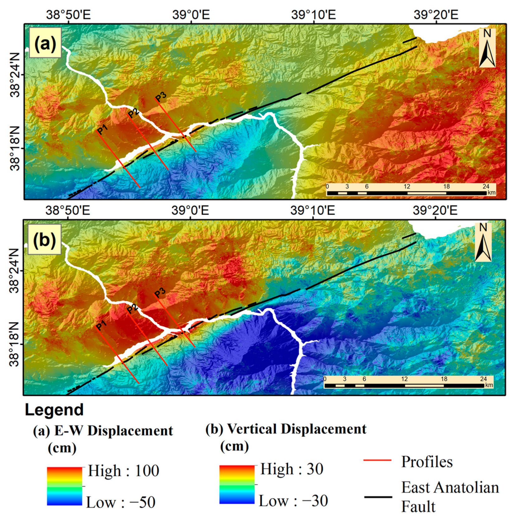
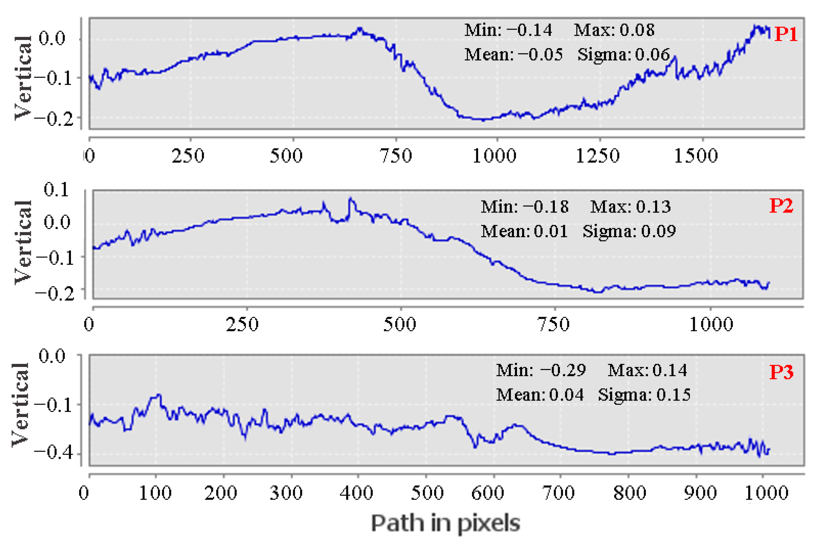
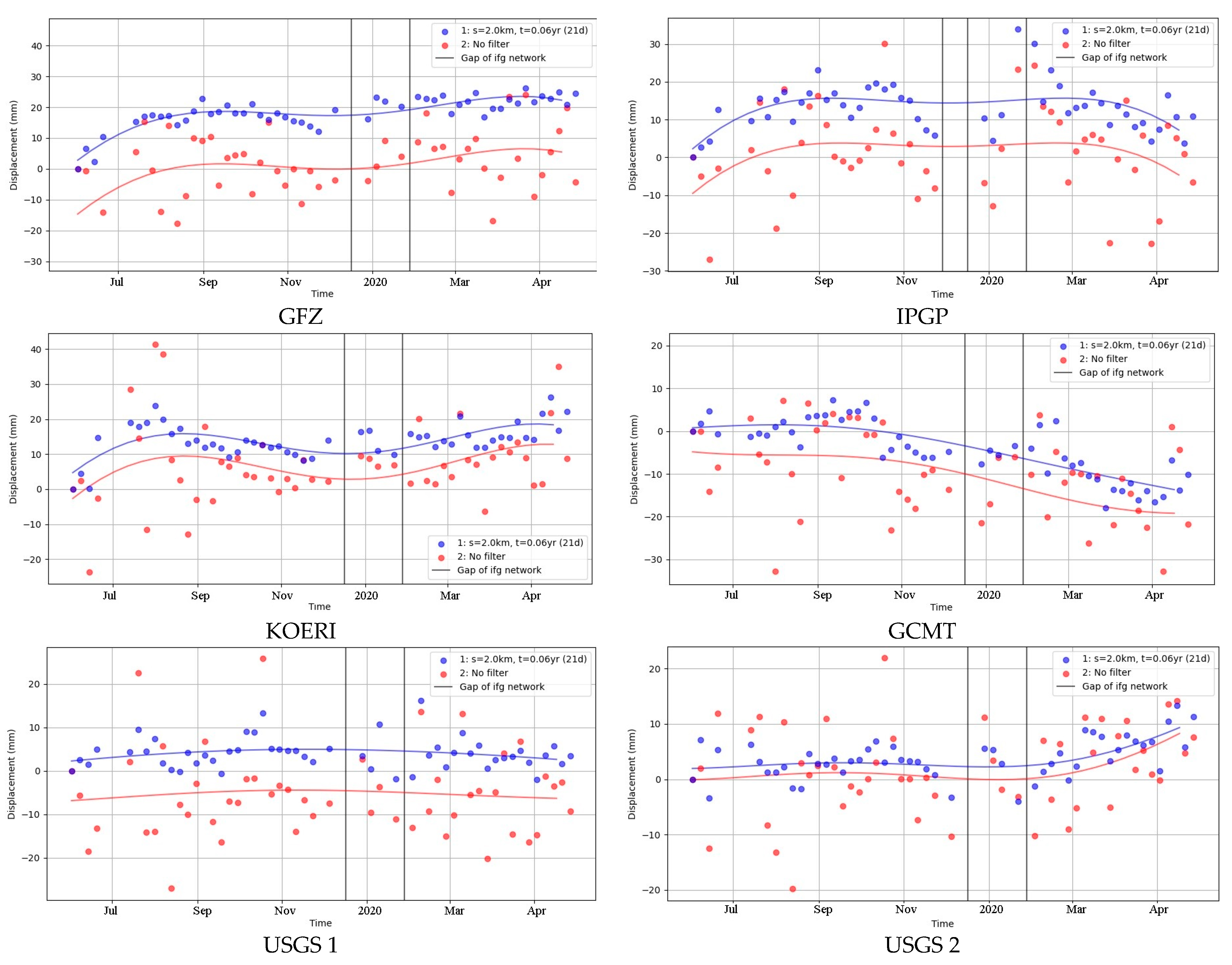
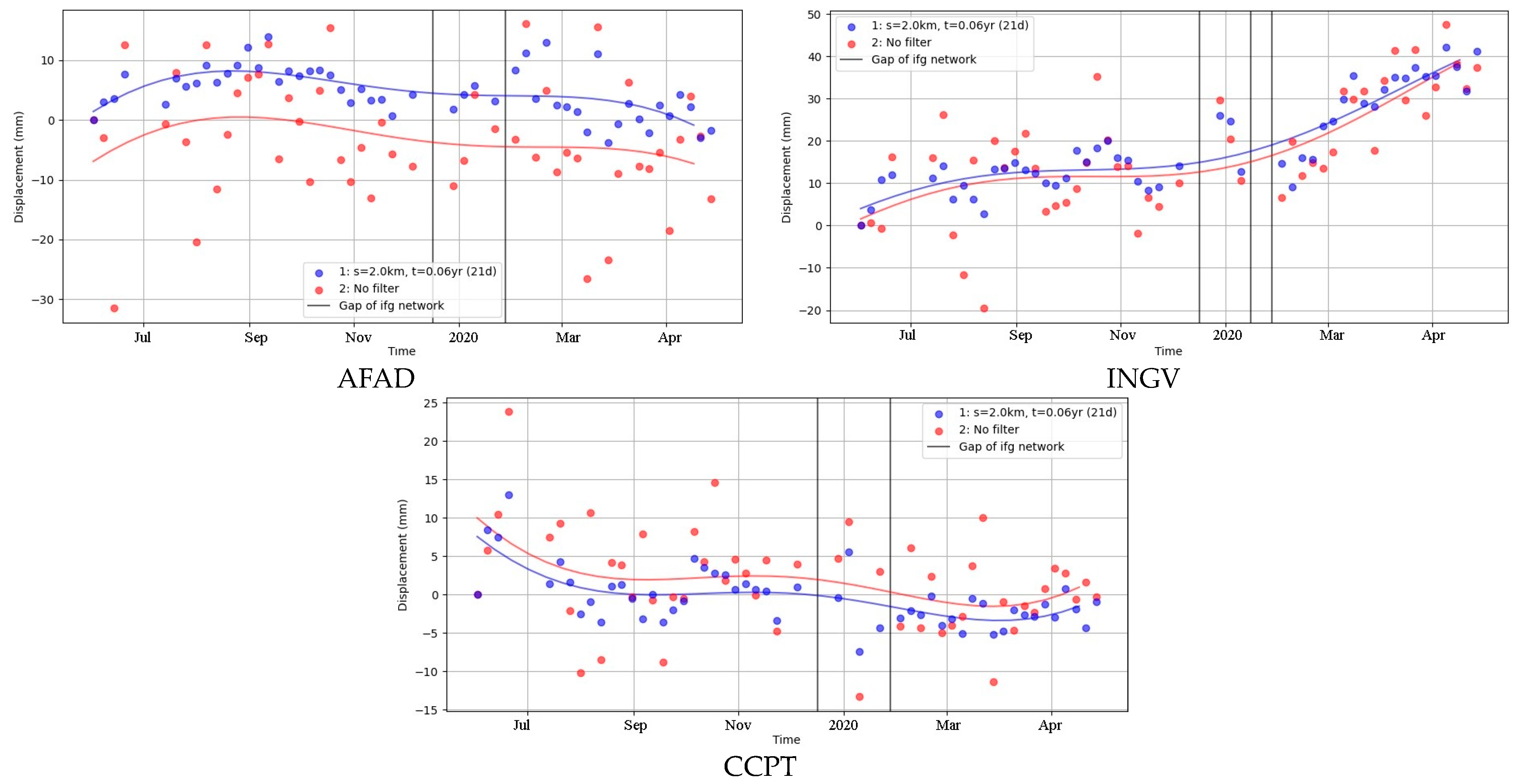
4.3. InSAR Deformations

The vertical and east–west displacement maps obtained from InSAR analysis are given in Figure 10. According to the results, shifts of up to 1 m in the west direction and up to 0.5 m in the east direction were detected (Figure 10a). The total deformation in the study area was up to 1.5 m. The vertical displacements were between −30 cm and 30 cm. The displacement profiles along the red lines on Figure 10 are presented together with statistical values such as min, max, mean, and sigma values in Figure 11. There is good concordance between the focal mechanism of the earthquake (Figure 6) and the results obtained from the InSAR analysis. The general character of the segments of the EAFZ is left-lateral strike-slip faults with a small vertical component.

Total vertical movement in the study area ranges between −30 cm and +30 cm (Figure 10b). There is a total deformation of 60 cm in the vertical direction. The displacement profiles along the red lines shown in Figure 10 can be seen in Figure 12 together with min, max, mean, and sigma values. The maximum displacement of 60 cm is similar to a result of the studies conducted by Bayık et al. [15], Cheloni and Akinci. [39], and Konca et al. [14] using similar methods and data.

Figure 13a,b show the cumulative displacement map in ascending and descending orbits for one year together with the epicenter locations given by different seismic stations; Figure 13c shows the land use land cover (LULC) map obtained from ESA WorldCover [40]. The area as shown in Figure 13c comprises mainly rangeland according to the ESA WorldCover product.

The time series analysis of ascending orbits on the epicenter locations is shown in Figure 14. Here, we used displacement values in ascending orbits due to the nearly-equal-to-vertical displacement in Figure 10b for the time series analysis shown in Figure 14. All epicenter locations except of KOERI were found in the rangeland according to the ESA WorldCover map (Figure 13c). The KOERI solution was located in a crop area. The blue dots in Figure 13 indicate filtered (high-coherence) solutions of InSAR. The IPGP, USGS-1, USGS-2, INGV, and CCPT solutions indicate sudden displacements around the time of the earthquake. The epicenters given by GCMT, IPGP, and GFZ are located on the south-east block while the others are on the north-west block (Figure 13a). The sudden displacements around the time of the earthquake were strongly related to the position of the epicenters because most of these points were located on the north-west block. However, there is no an agreement among the time series behaviors of the epicenter locations. The epicenters given by GCMT, IPGP, and GFZ are located on the south-east block while the others are on the north-west block (Figure 13a). It must be noted that some changes may also be associated with slope deformations, which requires further analysis.

5. Conclusions

In this study, we analyzed the epicenters determined for the Sivrice earthquake (26 January 2020) using aerial photogrammetry and InSAR time series analysis. We observed that almost all epicenters were not compatible with other seismic data. KOERI station is found to construct a good earthquake fault plane, but its location is out of the rangeland according to the ESA WorldCover map (Figure 13c). We suggest a review of the acquired seismic geographic data with the existing fracture data, as already carried out by some stations with human intervention, or by artificial intelligence tools followed and possibly finished by a human reviewer to minimize errors. We saw the valuable contribution of aerial photogrammetry with photos taken immediately after an earthquake occurs in a time period of few days after the event, and using, if necessary, digital image enhancement techniques.

The InSAR analysis results for horizontal and vertical displacements show agreements with the findings in the literature. According to the results, displacements of up to 1 m in the westward direction and up to 0.5 m in the eastward direction were revealed. The vertical displacements were between −30 cm and 30 cm. In addition, we analyzed the epicenter locations with time series, and observed sudden changes around the time of the event. The sudden displacements around the time of the earthquake are considered to be related to the position of the epicenters as they are located on the NW block. However, no agreement among the time series behaviors of the epicenter locations was found. The main reason for this different behavior is mainly due to the locations of the epicenters because the epicenters given by GCMT, IPGP, and GFZ are located on the SE block while the others are located on the north-west block. In future work, an in-depth analysis of the changes based on LULC can be performed to comprehend the sources of surface changes in different locations.

References

1. Taymaz, T.; Ganas, A.; Yolsal-Çevikbilen, S.; Vera, F.; Eken, T.; Erman, C.; Öcalan, T. Source mechanism and rupture process of the 24 January 2020 Mw 6.7 Doğanyol–Sivrice earthquake obtained from seismological waveform analysis and space geodetic observations on the East Anatolian Fault Zone (Turkey). Tectonophysics 2021, 804, 228745. [Google Scholar] [CrossRef]
2. Tatar, O.; Sözbilir, H.; Koçbulut, F.; Bozkurt, E.; Aksoy, E.; Eski, S.; Özmen, B.; Meti, Y. Surface deformations of 24 January 2020 Sivrice (Elazığ)–Doğanyol (Malatya) earthquake (Mw = 6.8) along the Pütürge segment of the East Anatolian Fault Zone and its comparison with Turkey’s 100-year-surface ruptures. Mediterr. Geosci. Rev. 2020, 2, 385–410. [Google Scholar] [CrossRef]
3. Günaydin, M.; Atmaca, B.; Demir, S.; Altunişik, A.C.; Hüsem, M.; Adanur, S.; Ateş, Ş.; Angin, Z. Seismic damage assessment of masonry buildings in Elazığ and Malatya following the 2020 Elazığ-Sivrice earthquake, Turkey. Bull. Earthq. Eng. 2021, 19, 2421–2456. [Google Scholar] [CrossRef]
4. Isik, E.; Aydin, M.C.; Buyuksarac, A. 24 January 2020 Sivrice (Elazig) earthquake damages and determination of earthquake parameters in the region. Earthq. Struct. 2020, 19, 145. [Google Scholar]
5. Atmaca, B.; Demir, S.; Günaydin, M.; Altunişik, A.C.; Hüsem, M.; Ateş, Ş.; Adanur, S.; Angin, Z. Field investigation on the performance of mosques and minarets during the Elazig-Sivrice Earthquake. J. Perform. Constr. Facil. 2020, 34, 04020120. [Google Scholar] [CrossRef]
6. Yurdakul, Ö.; Duran, B.; Tunaboyu, O.; Avşar, Ö. Field reconnaissance on seismic performance of RC buildings after the 24 January 2020 Elazığ-Sivrice earthquake. Nat. Hazards 2021, 105, 859–887. [Google Scholar] [CrossRef]
7. Bayrak, O.F.; Bikçe, M.; Erdem, M.M. Failures of structures during the 24 January 2020, Sivrice (Elazığ) Earthquake in Turkey. Nat. Hazards 2021, 108, 1943–1969. [Google Scholar] [CrossRef]
8. Sayın, E.; Yön, B.; Onat, O.; Gör, M.; Öncü, M.E.; Tunç, E.; Bakır, E.; Karaton, M.; Calayır, Y. 24 January 2020 Sivrice-Elazığ, Turkey earthquake: Geotechnical evaluation and performance of structures. Bull. Earthq. Eng. 2021, 19, 657–684. [Google Scholar] [CrossRef]
9. Nemutlu, O.F.; Balun, B.; Sari, A. Damage assessment of buildings after 24 January 2020 Elazig-Sivrice earthquake. Earthq. Struct. 2021, 20, 325. [Google Scholar] [CrossRef]
10. Caglar, N.; Vural, I.; Kirtel, O.; Saribiyik, A.; Sumer, Y. Structural damages observed in buildings after the 24 January 2020 Elazığ-Sivrice earthquake in Türkiye. Case Stud. Constr. Mater. 2023, 18, e01886. [Google Scholar] [CrossRef]
11. Cetin, K.O.; Cakir, E.; Ilgac, M.; Can, G.; Soylemez, B.; Elsaid, A.; Cuceoglu, F.; Gulerce, Z.; Askan, A.; Aydin, S.; et al. Geotechnical aspects of reconnaissance findings after 24 January 2020, M6. 8 Sivrice–Elazig–Turkey earthquake. Bull. Earthq. Eng. 2021, 19, 3415–3459. [Google Scholar] [CrossRef]
12. Karakas, G.; Nefeslioglu, H.A.; Kocaman, S.; Buyukdemircioglu, M.; Yurur, T.; Gokceoglu, C. Derivation of earthquake-induced landslide distribution using aerial photogrammetry: The 24 January 2020, Elazig (Turkey) earthquake. Landslides 2021, 18, 2193–2209. [Google Scholar] [CrossRef]
13. Yalcin, I.; Kocaman, S.; Gokceoglu, C. Production of Iso-Intensity Map for the Elazig Earthquake (24 January 2020) Using Citizen Collected Geodata. Int. Arch. Photogramm. Remote Sens. Spat. Inf. Sci. 2020, 43, 51–56. [Google Scholar] [CrossRef]
14. Konca, A.Ö.; Karabulut, H.; Güvercin, S.E.; Eskiköy, F.; Özarpacı, S.; Özdemir, A.; Floyd, M.; Ergintav, S.; Doğan, U. From Interseismic Deformation with Near-Repeating Earthquakes to Co-Seismic Rupture: A Unified View of the 2020 Mw6. 8 Sivrice (Elazığ) Eastern Turkey Earthquake. J. Geophys. Res. Solid Earth 2021, 126, e2021JB021830. [Google Scholar] [CrossRef]
15. Bayik, C.; Gurbuz, G.; Abdikan, S.; Gormus, K.S.; Kutoglu, S.H. Investigation of Source Parameters of the 2020 Elazig-Sivrice Earthquake (Mw 6.8) in the East Anatolian Fault Zone. Pure Appl. Geophys. 2022, 179, 587–598. [Google Scholar] [CrossRef]
16. Gokceoglu, C.; Sahmaran, M.; Unutmaz, B.; Aldemir, A.; Kockar, M.K.; Sandikkaya, A.; Icen, A. Preliminary Investigation Report on the 24 January 2020 Elazig—Sivrice Earthquake (Mw = 6.8); Civil Engineering Department, Engineering Faculty, Hacettepe University: Ankara, Türkiye, 2020; 45p. [Google Scholar] [CrossRef]
17. Gokceoglu, C.; Yurur., M.T.; Kocaman, S.; Nefeslioglu, H.A.; Durmaz, M.; Tavus, B.; Karakas, G.; Buyukdemircioglu, M.; Atasoy, K.; Can, R.; et al. Investigation of Elazig Sivrice Earthquake (24 January 2020, Mw = 6.8) Employing Radar Interferometry and Stereo airphoto Photogrammetry; Geomatics and Geological Engineering Departments, Engineering Faculty, Hacettepe University: Ankara, Türkiye, 2020; 51p. [Google Scholar] [CrossRef]
18. AFAD. T.C. İçişleri Bakanlığı, Afet ve Acil Durum Yönetimi Başkanlığı, 24 Ocak 2020 Sivrice (Elaziğ) Mw 6.8 Depremine İlişkin ön Değerlendirme Raporu; Deprem Dairesi Başkanliği: Ankara, Türkiye, 2020; p. 10s. (In Turkish) [Google Scholar]
19. Supporttolife. Elazig Earthquake Situation Report 3. 2020. Available online: https://reliefweb.int/sites/reliefweb.int/files/resources/200207_Turkey%20Earthquake_Sitrep3.pdf (accessed on 26 February 2020).
20. Kürçer, A.; Elmacı, H.; Yıldırım, N.; Özelip, S. 24 Ocak 2020 Sivrice (Elazığ) Depremi (Mw = 6.8) Saha Gözlemleri ve Değerlendirme Raporu; MTA Jeoloji Etüdleri Dairesi: Ankara, Türkiye, 2020; 48p. (In Turkish) [Google Scholar]
21. UltraCam Eagle M3. Available online: https://www.vexcel-imaging.com/brochures/UC_Eagle_M3_en.pdf (accessed on 5 August 2023).
22. Karakas, G.; Kocaman, S.; Gokceoglu, C. Comprehensive performance assessment of landslide susceptibility mapping with MLP and random forest: A case study after Elazig earthquake (24 January 2020, Mw 6.8), Turkey. Environ. Earth Sci. 2022, 81, 144. [Google Scholar] [CrossRef]
23. ESA Sentinel-1. Available online: https://sentinel.esa.int/web/sentinel/missions/sentinel-1 (accessed on 13 August 2023).
24. ESA SNAP. Available online: https://step.esa.int/main/toolboxes/snap/ (accessed on 13 August 2023).
25. Fattahi, H.; Agram, P.; Simons, M. A network-based enhanced spectral diversity approach for TOPS time-series analysis. IEEE Trans. Geosci. Remote Sens. 2016, 55, 777–786. [Google Scholar] [CrossRef]
26. Goldstein, R.M.; Zebker, H.A.; Werner, C.L. Satellite radar interferometry: Two-dimensional phase unwrapping. Radio Sci. 1988, 23, 713–720. [Google Scholar] [CrossRef]
27. Costantini, M. A novel phase unwrapping method based on network programming. IEEE Trans. Geosci. Remote Sens. 1998, 36, 813–821. [Google Scholar] [CrossRef]
28. Dalla Via, G.; Crosetto, M.; Crippa, B. Resolving vertical and east-west horizontal motion from differential interferometric synthetic aperture radar: The L’Aquila earthquake. J. Geophys. Res. Solid Earth 2012, 117. [Google Scholar] [CrossRef]
29. Morishita, Y.; Lazecky, M.; Wright, T.J.; Weiss, J.R.; Elliott, J.R.; Hooper, A. LiCSBAS: An open-source InSAR time series analysis package integrated with the LiCSAR automated Sentinel-1 InSAR processor. Remote Sens. 2020, 12, 424. [Google Scholar] [CrossRef]
30. COMET-LiCS Sentinel-1 InSAR Portal. Available online: https://comet.nerc.ac.uk/comet-lics-portal/ (accessed on 4 May 2021).
31. Lazecký, M.; Spaans, K.; González, P.J.; Maghsoudi, Y.; Morishita, Y.; Albino, F.; Elliott, J.; Greenall, N.; Hatton, E.; Hooper, A. LiCSAR: An automatic InSAR tool for measuring and monitoring tectonic and volcanic activity. Remote Sens. 2020, 12, 2430. [Google Scholar] [CrossRef]
32. Chen, Y.; Bruzzone, L.; Jiang, L.; Sun, Q. ARU-net: Reduction of atmospheric phase screen in SAR interferometry using attention-based deep residual U-net. IEEE Trans. Geosci. Remote Sens. 2020, 59, 5780–5793. [Google Scholar] [CrossRef]
33. Yu, C.; Li, Z.; Penna, N.T.; Crippa, P. Generic atmospheric correction model for interferometric synthetic aperture radar observations. J. Geophys. Res. Solid Earth 2018, 123, 9202–9222. [Google Scholar] [CrossRef]
34. Tavus, B.; Kocaman, S.; Nefeslioglu, H.A. Landslide detection using InSAR time series in the Kalekoy dam reservoir: Bingol, Türkiye. In Proceedings of the Image and Signal Processing for Remote Sensing XXVIII, Berlin, Germany, 5–6 September 2022; Volume 12267, pp. 218–226. [Google Scholar]
35. EMSC. Earthquake Moment Tensors. 2023. Available online: https://www.emsc-csem.org/Earthquake_data/tensors.php?date=2020-01-24 (accessed on 8 August 2023).
36. KOERI. Moment Tensor Solutions. 2022. Available online: https://www.frontiersin.org/articles/10.3389/feart.2022.945022/full (accessed on 10 May 2023).
37. USGS. W-Phase Moment Tensor (Mww), M 6.7–13 km N of Doğanyol, Turkey. 2022. Available online: https://earthquake.usgs.gov/earthquakes/eventpage/us60007ewc/moment-tensor?source=us&code=us_60007ewc_mww (accessed on 24 January 2020).
38. MTA. MTA Geological Maps, 1/500.000 Scale Geological Maps, Elazığ Sheet. 2022. Available online: https://www.mta.gov.tr/v3.0/hizmetler/500bas (accessed on 31 January 2017).
39. Cheloni, D.; Akinci, A. Source modelling and strong ground motion simulations for the 24 January 2020, M w 6.8 Elazığ earthquake, Turkey. Geophys. J. Int. 2020, 223, 1054–1068. [Google Scholar] [CrossRef]
40. Zanaga, D.; Van De Kerchove, R.; De Keersmaecker, W.; Souverijns, N.; Brockmann, C.; Quast, R.; Wevers, J.; Grosu, A.; Paccini, A.; Vergnaud, S.; et al. ESA WorldCover 10 m 2020 v100. 2021. Available online: https://zenodo.org/records/5571936 (accessed on 8 August 2023).
Figure 1. Locations and focal analyses of the main shock and aftershocks of the Elazig Sivrice earthquake published by AFAD [18].
Earth 04 00043 g001
Figure 2. Footprint (red polygon) of the aerial photogrammetric mission performed on 26 February 2020 by the HGM (map credit: HGM).
Earth 04 00043 g002
Figure 3. Perspective views of the DEMs, (a) with the orthophoto overlayed, and (b) color-coded.
Earth 04 00043 g003
Figure 4. InSAR time series analysis methodology for the assessment of displacement between June 2019 and June 2020.
Earth 04 00043 g004
Figure 5. Perpendicular baseline configuration and network of the interferograms from (a) descending and (b) ascending orbits. Red lines represent low-quality interferograms omitted from the dataset.
Earth 04 00043 g005
Figure 6. (A) Epicenter locations given by different seismic stations for the 24 January 2020 Sivrice earthquake. (B) Focal mechanism of the earthquake [35]. (C) Sketch showing how calculations are carried out. In (A), the yellow lines denote where the earthquake’s fault plane intersects with the topographic surface.
Earth 04 00043 g006
Figure 7. Linearity developed due to gas outflow from the surface rupture in the Euphrates River south of Ilincak Village (modified after [20]).
Earth 04 00043 g007
Figure 8. (A) Original view of the aerial photograph. ER: Euphrates River. (B) Digitally stretched image showing the light-colored lineament along the river channel. Numerical values are the radiometric values of the pixels used for piecewise linear stretching, e.g., values between 0 and 40 were stretched to 0 and 255. (C) Enlarged image of B. (D) Stepping lines detected along the river channel’s lineament. S: land sector of the study area. (E) Structural interpretation.
Earth 04 00043 g008
Figure 9. (A) Inset showing the location of (B), and (B) Google Earth satellite image showing the NE-trending lineaments, possibly of fault origin, NE of the river channel lineament studied. Several lineaments, marked by L, are visible on the water channel.
Earth 04 00043 g009
Figure 10. Displacements in (a) east–west and (b) vertical directions.
Earth 04 00043 g010
Figure 11. East–west displacement profiles along the lines (P1–3) shown in Figure 10 (in meters).
Earth 04 00043 g011
Figure 12. Vertical displacement profiles along the lines (P1–3) shown in Figure 10 (in meters).
Earth 04 00043 g012
Figure 13. (a) Displacement map in ASC orbit, (b) displacement map in DSC orbit, and (c) the LULC map obtained from ESA WorldCover.
Earth 04 00043 g013
Figure 14. Time series analysis results for the epicenter locations. Blue and red colors represent the filtered and unfiltered data, respectively.
Earth 04 00043 g014aEarth 04 00043 g014b