Article

Evaluation of Groundwater Potential Using Aquifer Characteristics in Urambo District, Tabora Region, Tanzania

by
Athuman R. Yohana
1,*,
Edikafubeni E. Makoba
2,
Kassim R. Mussa
2 and
Ibrahimu C. Mjemah
2
1
Ministry of Water, Lake Tanganyika Basin Water Board, Tabora Sub-Office, Tabora P.O. Box 307, Tanzania
2
Department of Geography and Environmental Studies, Sokoine University of Agriculture, Morogoro P.O. Box 3038, Tanzania
*
Author to whom correspondence should be addressed.
Earth 2023, 4(4), 776-805; https://doi.org/10.3390/earth4040042
Submission received: 16 July 2023 / Revised: 23 September 2023 / Accepted: 3 October 2023 / Published: 18 October 2023

Abstract

:
In developing countries like Tanzania, groundwater studies are essential for water resource planning, development, and management. Limited hydrogeological information on groundwater occurrence, availability, and distribution in Urambo District is termed a key factor that hinders groundwater development. This research was aimed at the evaluation of groundwater potential zones in a granitic gneiss aquifer in Urambo District by integrating six indicators (transmissivity, specific capacity, static water level, yield, total dissolved solids, and geology) that were developed and applied in the study area. The indicators were further combined, and a groundwater potential index map (GWPIM) was prepared using relative weights derived from the analytical hierarchy process (AHP). The results show that 67% and 27% of the study area are categorized as moderate and high groundwater potential zones, respectively. Groundwater is controlled by both Quaternary sediments (sands and gravels) and weathered to fractured granitic gneiss. Quaternary sediments host the major shallow aquifers (<35 m) with relatively high transmissivity, specific capacity, and yield (1.5 m2/day, 16.36 m2/day, and 108 m3/day, respectively). Granitic gneiss is not strongly fractured/weathered and forms an aquifer with a relatively low yield of about 10.08 m3/day. The findings were validated using three boreholes, and the results are consistent with the developed GWPIM. Such findings are of great importance in groundwater development as the techniques applied can be extended to other areas in Tanzania as well as other countries that experience similar geological environments.

1. Introduction

Globally, it is estimated that about 26% of the population has no access to safe and clean water [1]. Population growth and climate change have largely increased water demand, forcing the utilization of groundwater as the main alternative water source for domestic purposes [2,3]. Exploration and well drilling are the most common interventions to extract this resource. Unfortunately, limited understanding of the complex groundwater system has resulted in lower success rates for drilling groundwater production wells, particularly in developing countries.
In sub-Saharan Africa, most people depend on water from rivers, streams, lakes, and ponds for socio-economic purposes [4]. These sources are largely affected by pollution, a likely result of anthropogenic activities [5]. Hence, it appears that the solution to the problems of these sources lies basically in the efficient utilization of groundwater and the efficient management of aquifers, hand-dug wells, and boreholes [6].
In Tanzania, groundwater serves more than 25% of the population for drinking, irrigation, and industrial activities [7]. Over the past 24 years, there has been a tremendous increase in the number of newly developed boreholes in regions with high population growth, such as the cities of Dar es Salaam and Arusha [3]. Despite the fact that groundwater in the country is inadequately explored [5], the country is likely to have potential for groundwater. For instance, there are some boreholes with yields of about 460 m3h−1 in the semi-arid region of Dodoma [8], and in the Pangani basin, the yield of boreholes ranges between 10 and 800 m3 h−1 [9].
In Urambo District, there are limited surface water sources, and the local people depend solely on groundwater [10]. Groundwater is not well explored, and there is limited hydrogeological information on groundwater occurrence, availability, and distribution within the study area. Due to the overdependence on groundwater in Urambo District as a result of inadequate public water supply, it is essential to evaluate the potential of groundwater for proper management and development for the population of the study area due to the fact that the majority of people and towns use groundwater for home and some agricultural purposes. According to [11], a typical barrier to efficient groundwater management in the study area resulted from a poor understanding of groundwater resources and the heterogeneity of groundwater occurrence in the complex basement terrain. Thus, there is a need to evaluate the groundwater potential in Urambo District.
The major hydrogeological works that have been carried out in the study area are the work completed by the Japanese International Cooperation Agency (JICA). In the year 2011, 11 boreholes were drilled in the study area by the Rural Water Supply Project in the Tabora region. In this project, about 91% of the drilled boreholes were not productive, and the few productive boreholes were characterized by low yields averaging 10.08 m3/day [12]. The findings indicated that barren boreholes were associated with crystalline rocks in high altitude areas, and this indicated that the employed exploration techniques were vertical electrical sounding (VES) and electrical resistivity tomography (ERT). Productive boreholes (although their yield was low) were found to be associated with sand and gravel.
The borehole distribution indicated that most of the barren boreholes were centered in basement rocks and productive boreholes were located in swamps and the low altitude areas. Such findings provide preliminary information that guides groundwater exploration in the study area.
Studies on aquifer properties can be used to provide more reliable information on the aquifer characteristics of the formation that controls groundwater occurrence, storage, and movement [5,11,13,14,15,16]. The pumping test is one of the most effective methods for determining the hydraulic properties of the water-bearing layers simply because it allows for the quantification of groundwater and hydraulic conductivity, both of which depend on porosity, specifically the secondary porosity in the hard rock aquifer formation [15]. In areas with hard rocks and more exposed fractures and weathered formations, pumping tests are usually carried out as one of the hydraulic studies for assessment of the aquifer’s performance [16].
Different methods, such as Theis (1935), Cooper–Jacob (1946), Neuman (1972), and Walton’s (1962), have been proposed to evaluate aquifer properties in both confined and unconfined aquifers. When a pumping test is conducted without an observation well, the Cooper–Jacob (1946) straight line method is commonly used to evaluate groundwater potentiality due to its simplicity, low cost, and the fact that it can give the true formation parameters [17,18].
In Urambo District, the groundwater supply potential and its spatial distribution are inadequately known, mainly due to their hydrogeological complexity. This has led to improper sitting and drilling of productive boreholes within the study area, thus wasting the meager financial resources that would otherwise be allocated to other sectors of development.
This study therefore aims to evaluate the groundwater potential in Urambo District so as to provide reliable and vital hydrogeological information that will help in the exploration, planning, and management of groundwater resources in the district.

2. Materials and Methods

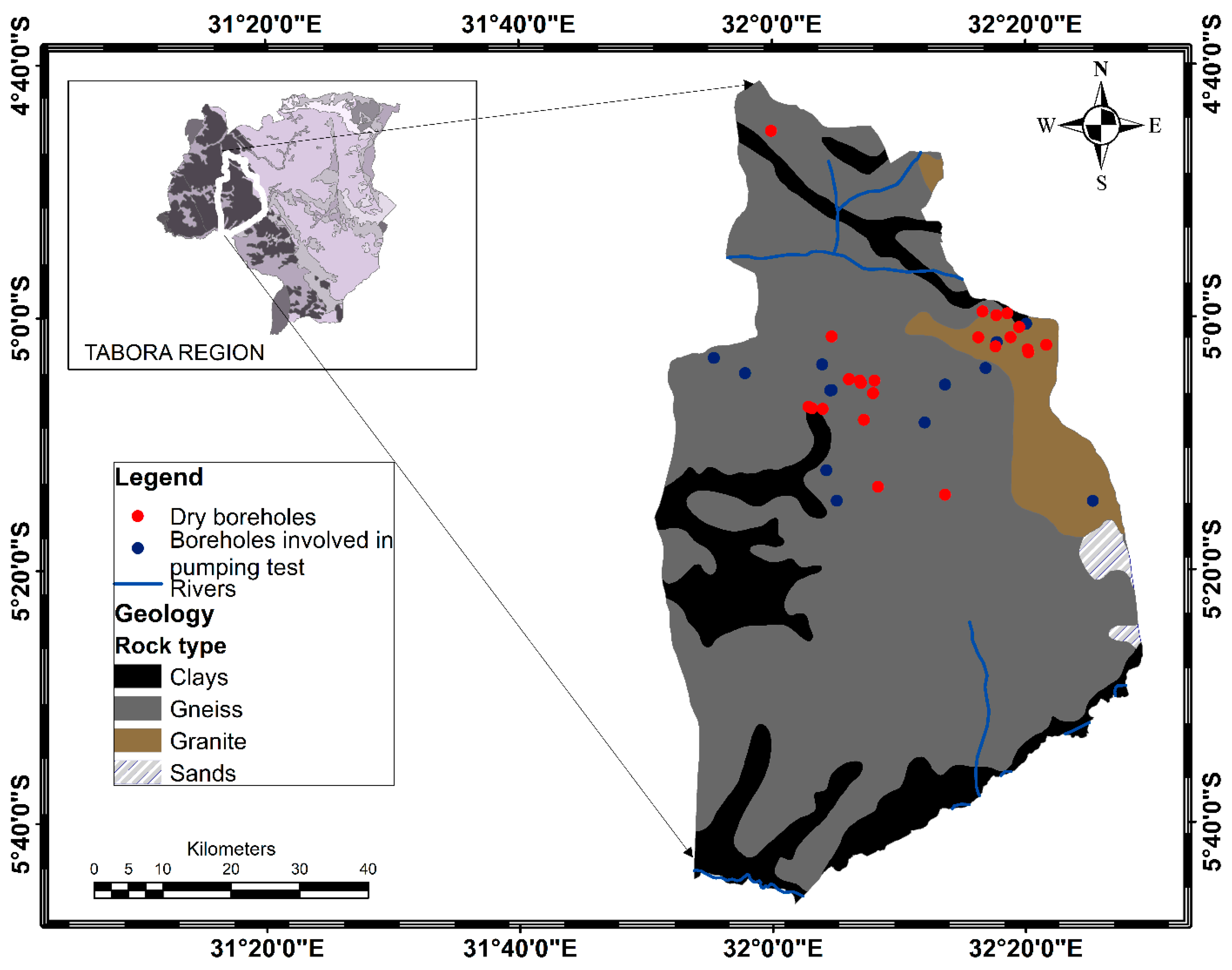
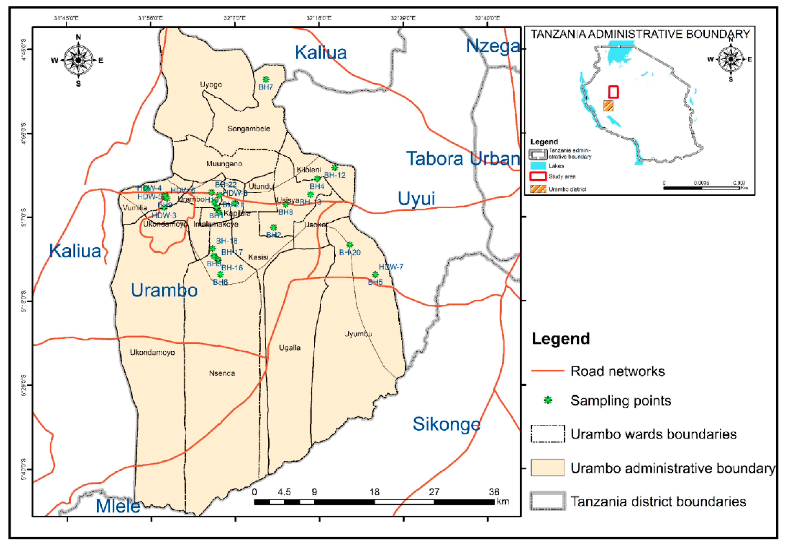
2.1. Description of the Study Area
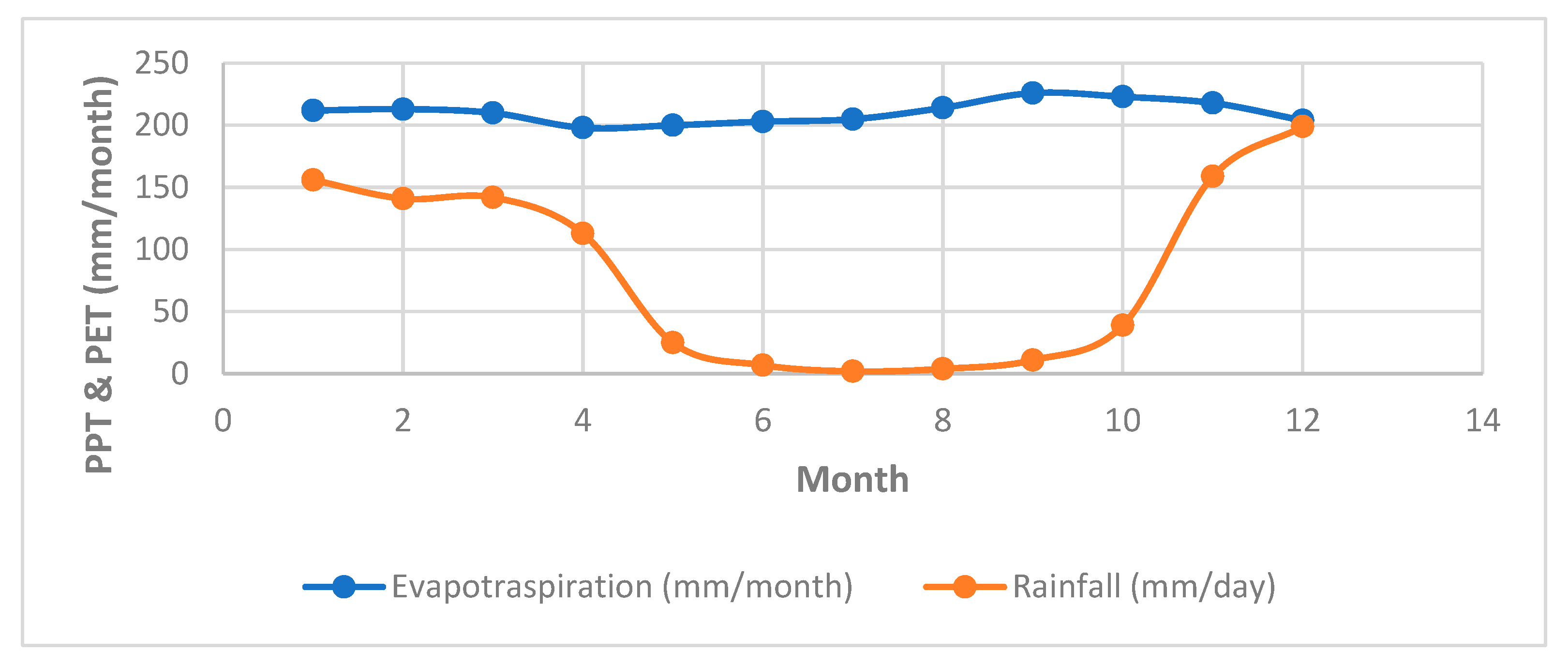
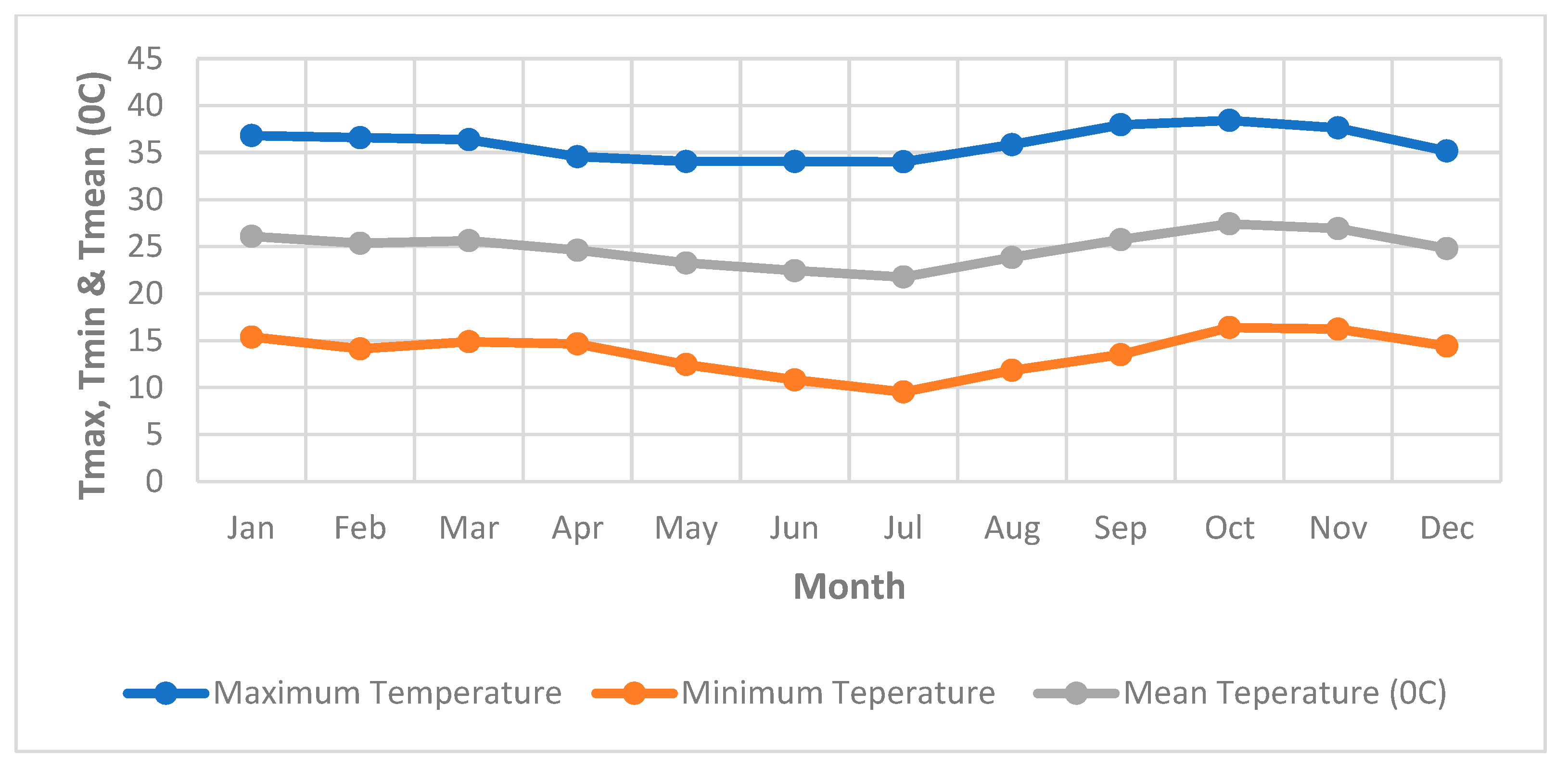
The study area is located in the northwestern part of Tanzania, in the Tabora region, between latitudes 4.69°–5.81° S and longitudes 31.82°–32.45° E (Figure 1). It covers an area of 6110 km2 [19] with an elevation varying from 1000 to 1500 m [20]. The study area is accessible throughout the year by Tabora to Kigoma Road in the town center and on rough roads in the surrounding areas.

2.2. Climate

Urambo district receives a relatively low amount of rainfall of about 997 mm/year (https://power.larc.nasa.gov/data-access-viewer/, accessed on 15 September 2023). The main rainy season is between November and May, with dry spells between June and October [11] (Table 1). Based on climatic data for 20 years (2001–2021) and potential evapotranspiration (PET) estimation using the Hargreaves–Samani (HS) method, the area has a high PET of approximately 2525 mm/year (Table 1) (Figure A1 in Appendix A). The study area had only one weather station with inconsistent data records, so the study opted to use meteorological datasets from the National Aeronautics and Space Administration (NASA) due to their quality of data with a resolution of 0.5 × 0.625-degree lat/long region = 1097.84 m. This has also been reported by other researchers [21].
On average, the area exhibits a semi-arid climatic condition (aridity index of 0.4) (Table 1), with patches of humid conditions in January, February, and March. Nevertheless, from May to October, it is generally dry, with an aridity index ranging between 0.12 and 0.17 (Table 1), which literally indicates arid or hyper-arid conditions (Table 2).
The monthly average temperature ranges between 14 and 36 °C with a mean monthly temperature of 25 °C (Table 1). The highest average monthly temperature occurs between September and April, with the peak at about 38 °C in October, just before the beginning of the wet season, while minimum temperatures occur between May and August, with a peak of about 10 °C. (Figure A2 in Appendix A).

2.3. Geology and Hydrogeology

Geologically, Urambo district is largely characterized by Archaean crystalline basement rocks of the Dodoman system which is the oldest stratum in Tanzania (~4000–2500 Ma [22]). It is largely composed of metamorphic rocks (gneiss, amphibolite, migmatite, and schist) and intrusive rocks (granite and granodiorite) which are distributed in the vast area of the eastern part of the district [12,23] (Figure 2). Within the study area, most of the low land areas/depressions are characterized by lacustrine sediments and old alluvium (Pleistocene) to recent alluvium (Quaternary age grading from clays to sands). Generally, the age of these sediments ranges between 0 and 2.58 Ma [22]. Major tectonic events in the study area are related to the intrusive events that led to the formation of granite and granodiorite. Other recent tectonic activities are associated with the East Africa Rift System which is sub-parallel to the faults that make up the basement [12]. These faults are primarily formed in the north–south and northwest–southeast directions of the basement [12].
The groundwater potentiality in the study area is generally low because of the low permeability of the common gneissic and granitoid rocks in the study area. However, there is increased groundwater potentiality in a few specific areas where weathering is relatively high or rocks are structured [24]. There is shallow groundwater occurrence in low land areas that are covered by sediments. However, most of these areas are dominated by clays (Figure 2), which overlay the basement rocks. Both clays and basement granitoid to gneissic rocks are characterized by relatively low permeability [23]. This lowers the groundwater potentiality in the areas. Groundwater potentiality is likely to increase in depression areas where alluvial sediments are grading to coarse sands and gravels, forming shallow aquifers.
Within the study area there are limited ephemeral streams that fall under the Malagarasi catchment with three major tributaries: the Igombe, Ugalla, and Wara rivers [12]. These streams can recharge the surrounding areas during the rainy season, depending on the porosity and permeability of the surrounding geological materials. Thus, the potential recharge is expected to be regional, and, in most cases, such recharges are likely to favor deep aquifers [25]. However, this is contrary to the study by [24], which indicated that groundwater in some specific areas is controlled by weathered zones [26].

2.4. Data Collection

In order to evaluate groundwater potential in the area, a pumping test was conducted involving 15 boreholes (Figure 2), followed by physical parameter measurements using a Wangtech multi-parameter instrument. The primary data were supported by the secondary data which were borehole logs from the Lake Tanganyika Basin Water Board, Tabora Sub Office.

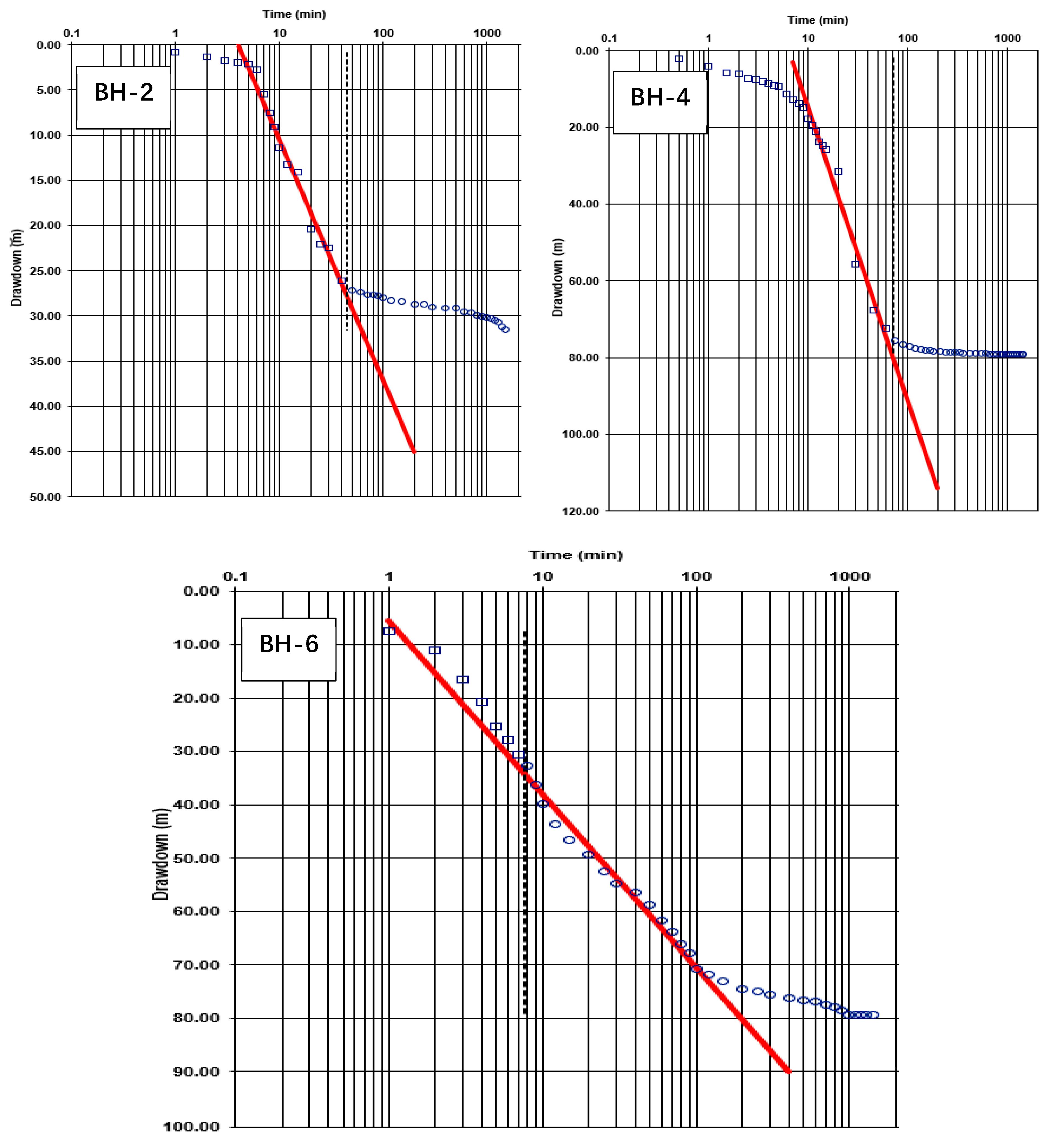
2.4.1. Execution of Pumping Tests

The pumping tests were carried out in 15 boreholes for the evaluation of aquifer properties (transmissivity and specific capacity). Before the pumping tests, important borehole data such as borehole depth, static water level, well diameter, and location were measured. Both step and constant pumping tests were implemented in all boreholes without an observation well. Specifically, the step test aims at determining the discharge that is within the well aquifers’ yield limits, which can be tested by a continuous constant pumping test [18,19,26]. All boreholes had a diameter of 6 inches and depths ranging between 25 and 150 m. Thus, a submersible pump with a capacity of 5.5 HP was used. During the constant rate of pumping, the drawdown (water level response) and the time were measured and recorded using an electric dipper and stopwatch, respectively. The flow rate of water pumped from the borehole was measured immediately after starting the pumping test, and the measurements were repeated at different time intervals using a bucket of known volume (22 L). On average, equilibrium was attained after 360 min (6 h) to 1440 min (24 h). Recovery time was measured at the same intervals as those used to measure drawdown until it attained approximately its original static water level.

2.4.2. Water Sample Collection and Measurement of Physico-Chemical Parameters

A total of 30 wells (22 boreholes and 8 hand-dug wells) were sampled in May 2022 using standard procedures as reported by [27]. In situ measurements of physical parameters such as total dissolved solids (TDS), dissolved oxygen (DO), temperature, pH, turbidity, and electric conductivity (EC) were carried out using the Wangtech multi-parameter. Equipment calibration was carried out prior to taking the measurements.

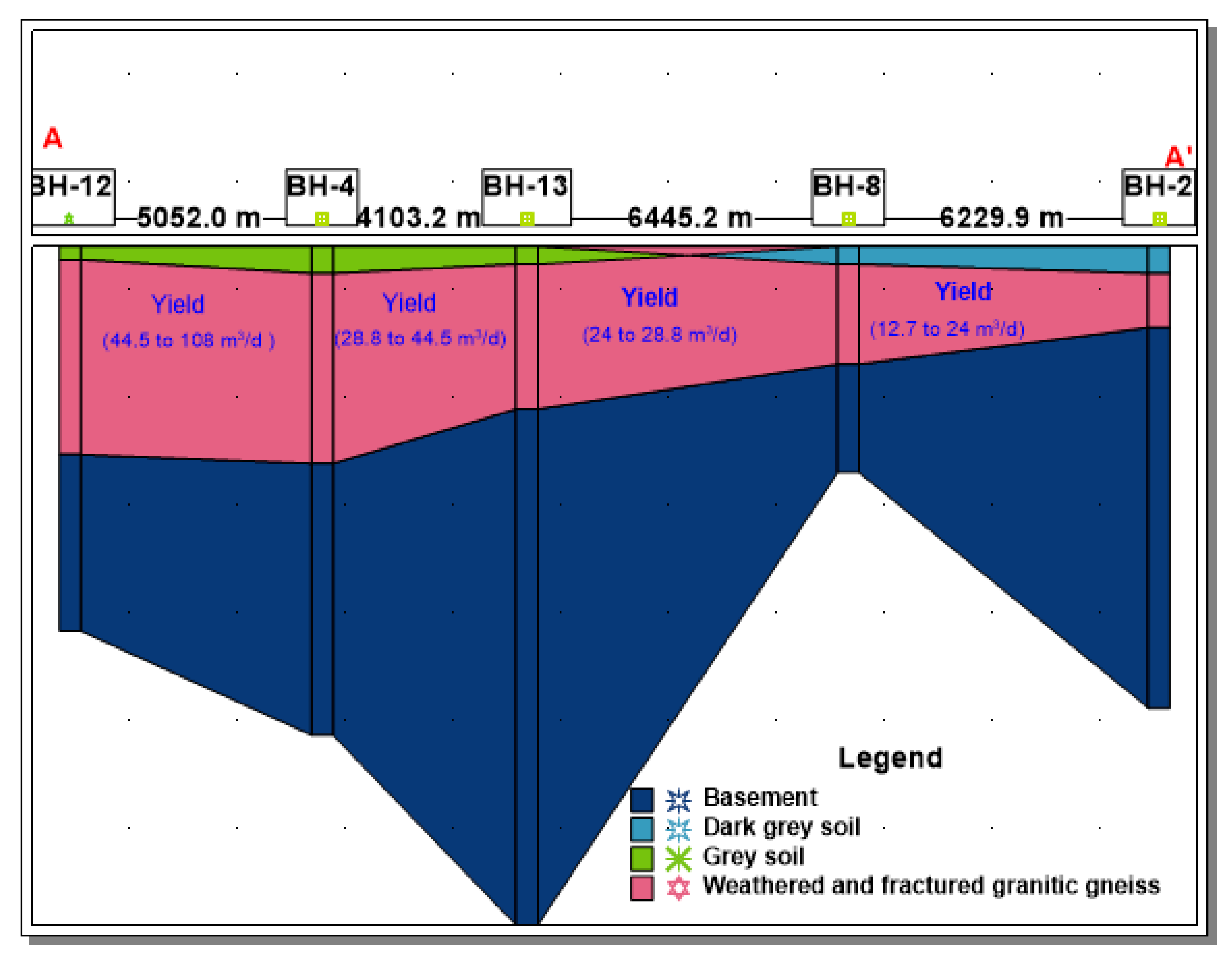
2.4.3. Lithology and Hydrogeological Cross-Section

The borehole drill cuttings (chips) at 2 m intervals were logged based on visual inspection of the samples. Key parameters in relation to groundwater occurrence, which are rock types, the degree of weathering, color, grain size, the degree of sorting, and the development of secondary minerals, were documented. The developed lithological logs were further used to construct three hydrogeological cross-sections using Strater 5 software.

2.5. Pumping Test Analysis and Interpretation Methods

The Cooper and Jacob method, a common method for the evaluation of pumping test data [27,28], was employed to evaluate transmissivity and specific capacity in the study area. A semi-logarithmic paper was used to plot the graph of drawdown against the elapsed time during the pumping test. Analysis with the Cooper and Jacob method involved the best-fitting straight line to the drawdown data plotted [29]. The early points were ignored during fitting because they are known to be affected by the volume of water that was stored in the borehole [30]. Thus, the middle and/or latter points were considered during the fitting of the line.
The discharge rate (m3/day) during the pumping test and the slope (∆s), which is the change in drawdown of one logarithmic cycle, were determined and assimilated into the Cooper and Jacob well flow equations for the determination of transmissivity (T) and specific capacity (Sc) (Equations (1) and (2), respectively).
T = 2.3 Q/(4π∆s)
where Q and ∆s stand for the constant pumping rate (m3/day) and drawdown difference per one log cycle (m), respectively, while specific capacity was calculated using the ratio of discharge to drawdown as shown in Equation (2).
Sc = Q/∆s
Transmissivity and specific capacity values are commonly integrated together to assess groundwater potentiality [14]. Inverse distance weighting (IDW), kriging, and trend surfaces are among the prediction approaches used in spatial interpolation for a given dataset, but their effectiveness has not been consistently demonstrated by any consistent findings [30]. Some researchers discovered that the Kriging method outperformed IDW and other methods due to the careful selection of the ideal number of neighboring points as well as the variogram model and its parameters. However, other researchers found that kriging was not superior to the other methods, as reported by [31]. Hence, selecting the right spatial interpolation approach for a given dataset is normally difficult. In this study, these parameters (transmissivity and specific capacity) were interpolated using inverse distance weighting (IDW) in Arc GIS Version 10.5 to generate the spatial map.

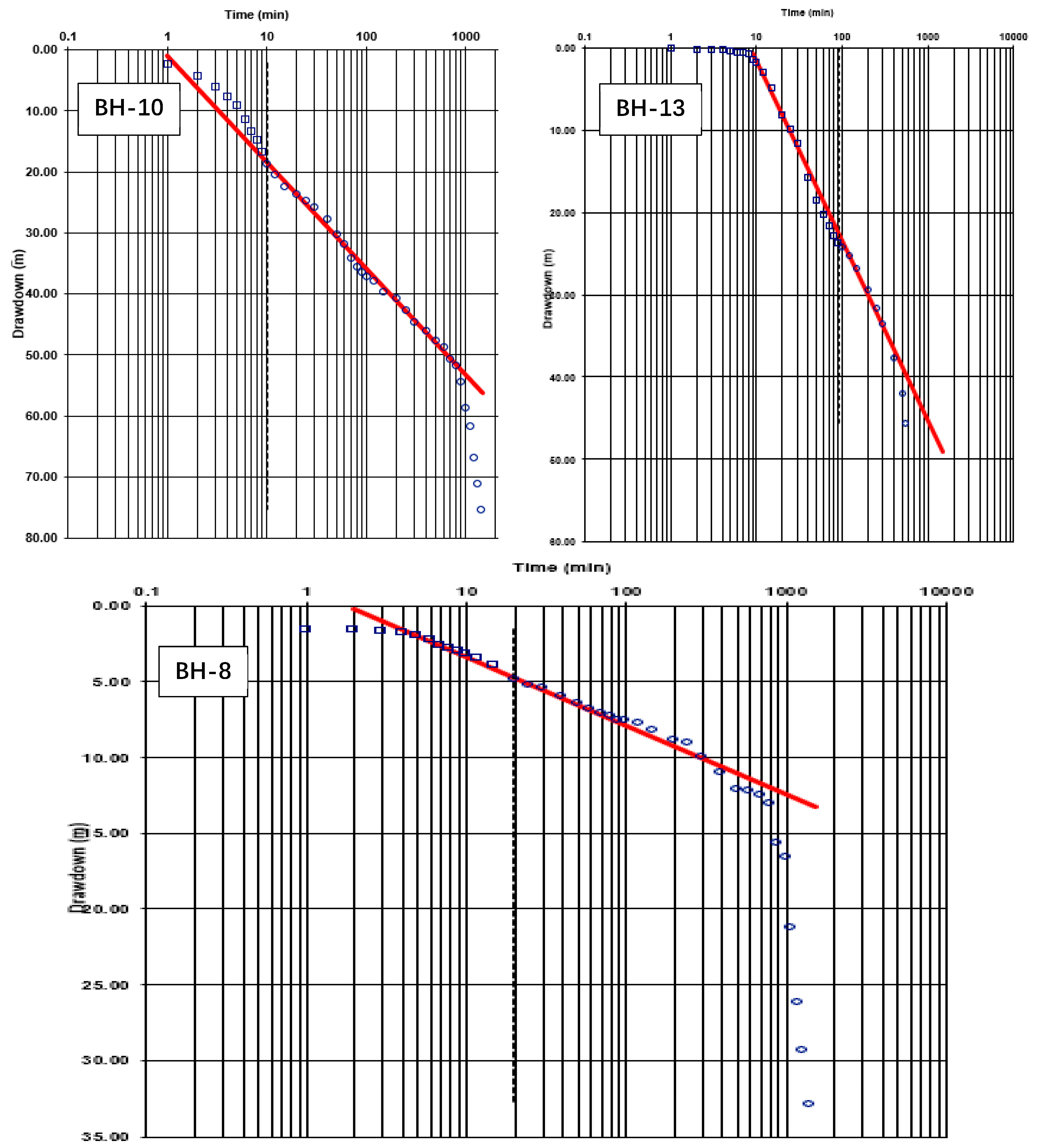
2.5.1. Transmissivity Analysis

Two methods were involved in the transmissivity analysis. The first method was descriptive statistical testing, which is commonly used in assessing transmissivity [14,17,18,30,31,32]. With this method, transmissivity values were assembled together and then the transmissivity index was calculated using Equation (4).
T = 10Y−8.96 × 86400
Equation (3) may be rearranged to obtain Equation (4)
Y = Log (T/86400) + 8.96
where Y—transmissivity index.
The second method is Krasny’s classifications; this approach considers a transmissivity classification system based on transmissivity magnitude, variation, and index values as proposed by [33] (Table 3, Table 4 and Table 5). These classification methods are presented in Table 3, Table 4 and Table 5. However, this classification left out other details. For that matter, therefore this study created another classification which yielded five classes: very low, low, high and very high.

2.5.2. Specific Capacity

The specific capacity of a well is simply the pumping rate (yield) divided by the drawdown (Equation (5)). It is a very valuable number that can be used to provide the design pumping rate or maximum yield for the well. It can be used to identify potential well, pump, or aquifer problems and can be used accordingly to develop a proper well maintenance schedule [27]. In this study, specific capacity was estimated in 15 pumped boreholes.
Sc = Q/∆s
where Sc = specific capacity (m2/day)
Q = constant pumping rate (m3/day)
∆s = unit drawdown

2.6. Charactrizaion of Physical Parameters in the Water Samples

All generated physical parameters were analyzed statistically using descriptive statistical methods, particularly mean values, and the values were compared with national and international standards. Furthermore, Arc GIS Version 10.5 was employed to assess the spatial distribution of these values.

2.7. Lithological Log Analysis and the Development of Cross-Sections

The lithological logs collected from the Lake Tanganyika Basin Water Board were first validated by re-logging a few existing rock chips stored in chip trays in the Tabora Water Office. Thereafter, the logs were subjected to Strata 5 software, which requires general lithological logs, complex lithological logs (geological stratigraphic formations with known thickness), and the depth of the well. This information was arranged in accordance with the software requirements (tables of depth, lithological logs, complex lithological logs, and well construction) and was integrated into the Strater 5 software to attain the well design and finally the hydrogeological cross-section of the selected boreholes. Three cross-sections were developed based on the borehole proximity, geology (boreholes located in different geological units), and depths for reliable interpolation of lithological units.

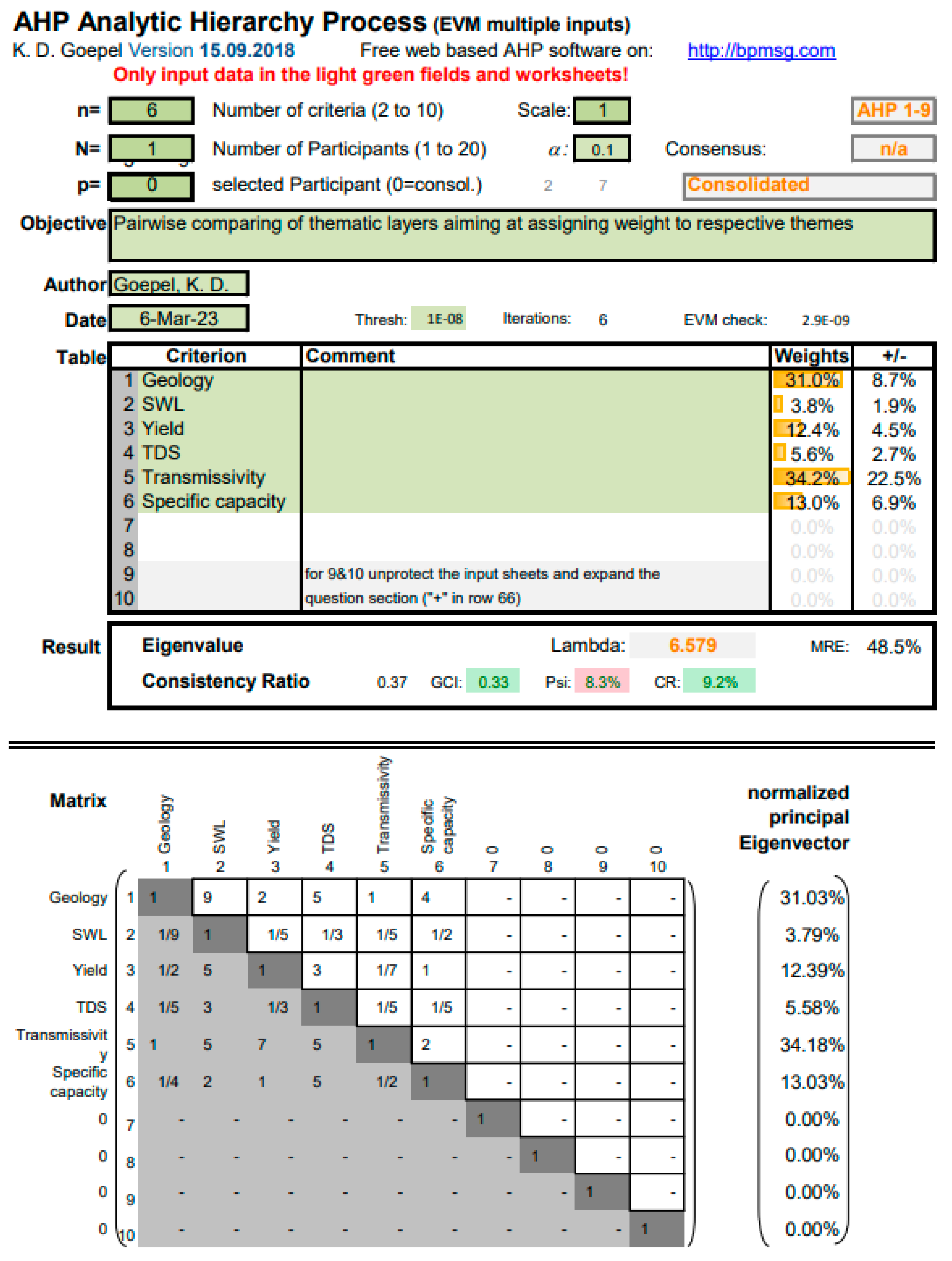
2.8. Integration of Datasets for Assessing Groundwater Potentiality

Pumping test parameters, including transmissivity, specific capacity, yield, static water level, TDS, and geology, were processed into six thematic maps. The analytical hierarchy process (AHP) technique was adopted in the calculation of the percentage of influence based on the user’s awareness of the importance of the thematic layers to groundwater potential. AHP is the most popular technique pioneered in the identification of groundwater potential zones, it is one of the most effective instruments for making decisions, and the outcomes are frequently trustworthy [34]. It breaks down complex choices into a series of pair-wise comparisons and integrates the outcomes, as well as minimizing biases in the decision-making process.
By using the AHP technique, the weight was assigned to each parameter by comparing a pair of matrices at a consistency ratio (CR) of 0.09, which meets the consistency criteria for pair-wise comparison with CR ≤ 0.1 [34]. The scale factor in AHP, which depends on the user’s selection, was used to categorize the thematic layers into classes. The scale value represents the importance of the individual features in a layer, whereas influence (weight) represents the layer’s overall importance. The values on the scale ranged from 1 to 5. Based on the classes of the thematic layers, each layer was given a ranking from 1 to 9, a large value representing a higher influence on groundwater potential and vice versa.
The groundwater potential index map (GWPIM) was then constructed by overlaying six thematic layers (transmissivity, specific capacity, yield, static water level, TDS, and geology) using the overlay function in GIS. The generated map was validated using three boreholes drilled in December 2022 in the study area.

3. Results

3.1. Physico-Chemical Parameters in the Water Samples

The descriptive statistics of the physicochemical parameters of the analyzed water samples are summarized in Table 6 hereunder.
Turbidity varies from 0.0 to 218 NTU (mean = 33 NTU). The mean value is high relative to the WHO recommended value of 5.00 NTU. This is largely attributed to elevated values at (BH-4, BH-5, BH-7, BH-13, HDW-I, HDW-2, HDW-3, HDW-4, and HDW-5) (Table 6). With the exception of BH-20, BH-15, and BH-14 with pH values between 6.4 and 6.85, all other sampled water was slightly alkaline with pH values between 6.4 and 8.5., which are within the permissible limits of 6.5 to 8.5 [35] and 6.5 to 9.2 [36].
In this study, the electrical conductivity values demonstrated a wide range between 60 to 3762 μS/cm (mean = 770 μS/cm) (Table 6 and Figure 3 refer). Approximately 17.24% of the samples had values beyond the maximum permissible limit of the WHO standard for drinking water. These boreholes are BH-14, BH-22, BH-1, BH-19, BH-2, BH-8, and BH-9. According to WHO standards, EC value should not exceed 400 μS/cm and 1000 μS/cm for TBS [36]. These results clearly indicate that the water in the study area was considerably ionized and has slightly high level of ionic concentration activity due to relatively high dissolved solids (Table 6).

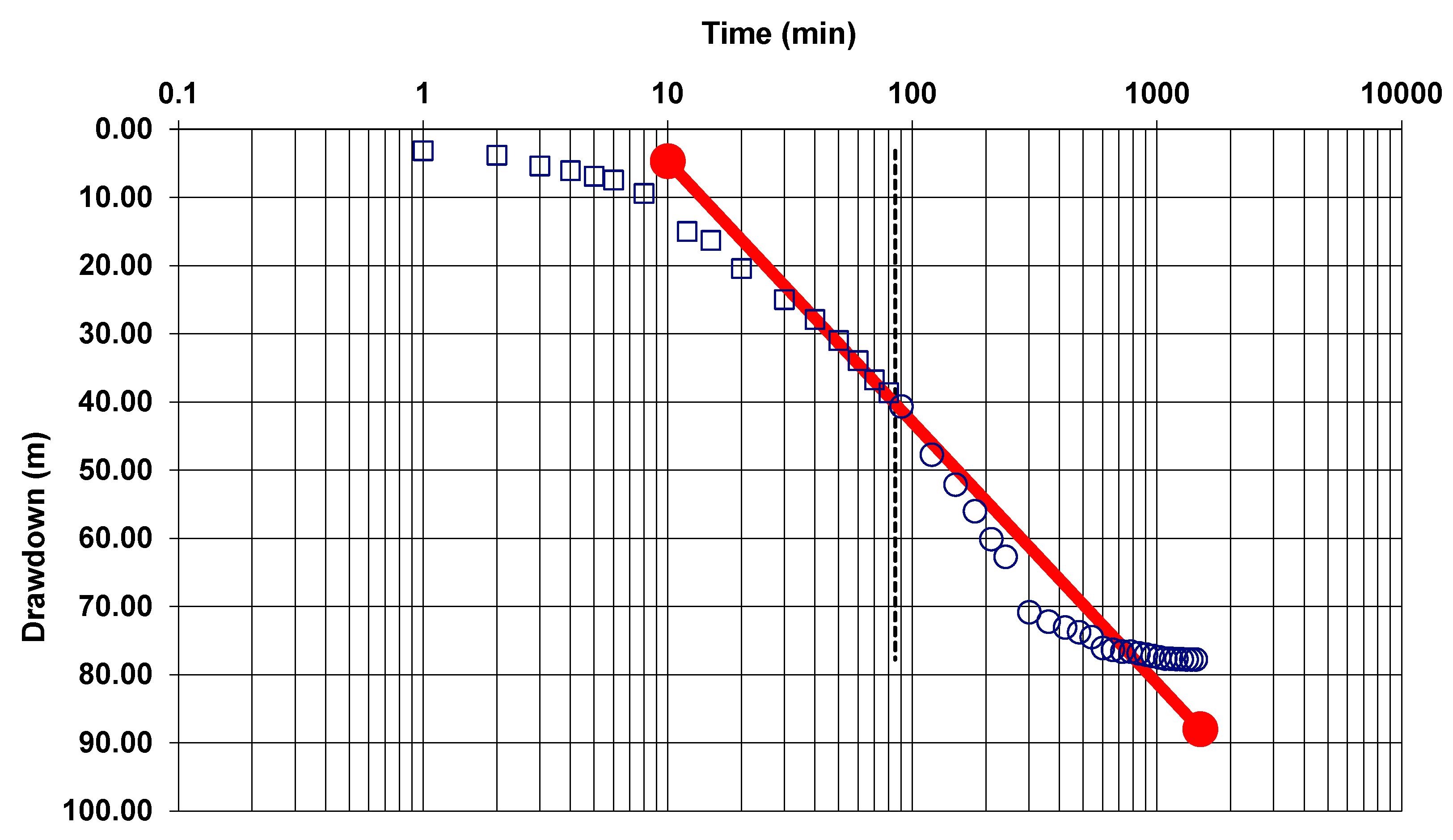
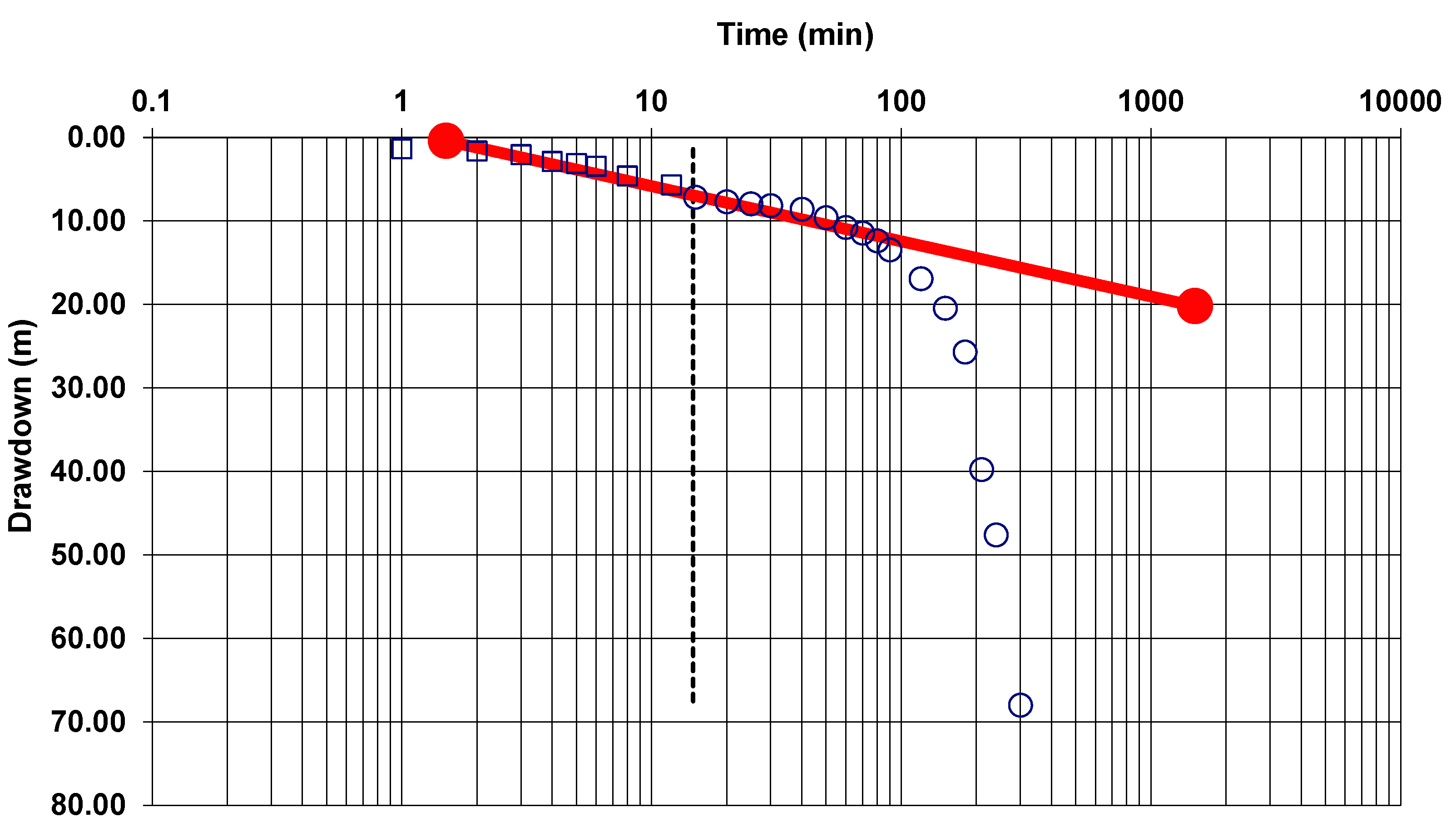
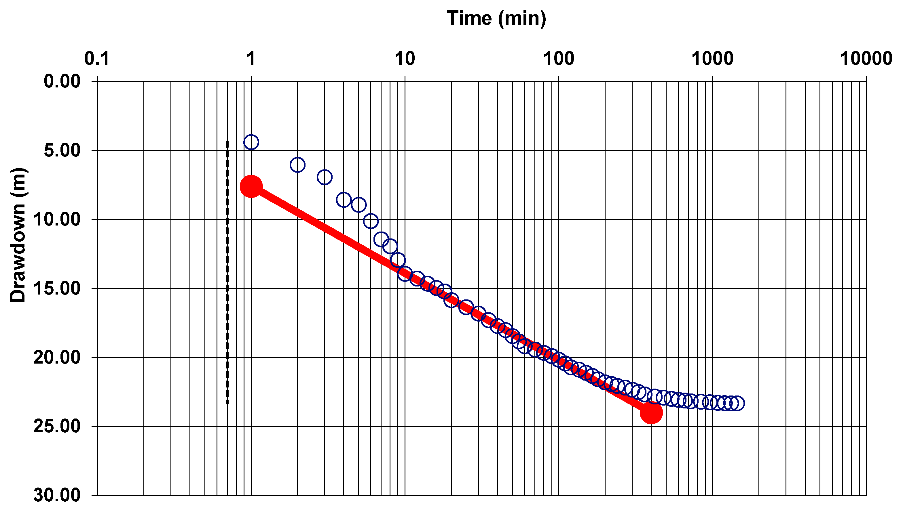
3.2. Pumping Test Results

The pumping test results (static water level, yield, transmissivity, and specific capacity) for 15 boreholes are presented in Table 7. Transmissivity and specific capacity were obtained from Cooper and Jacob graphs.
The drawdown values computed after the pumping test (Table 7) were between 4.47 and 44.27 m with a mean value of 20.35 m. In general, the average drawdown value of 20.35 m indicates that the aquifers in the study area are generally poor in terms of both recharge and discharge, pointing to low permeability [37].
The pumping test results for BH No.3 (Figure 4) are closely related to the results of boreholes BH-2, BH-4, and BH-6 (Table 7). All display gentle deflection of time-drawdown data on the left side (latter data) of the Cooper–Jacob straight line method (Figure A4 in Appendix B).
The pumping test results for BH No. 12 (Figure 5) are closely related to the pumping results for boreholes BH-8, BH-10, and BH-13. They are characterized by sharp deflection of time-drawdown data to the right side (latter data) of the Cooper—Jacob straight line method (Figure A5 in Appendix B).
The pumping test results for the Kichangani borehole (Figure 6) are closely related to the pumping results for boreholes BH-2, BH-4, and BH-6. They are characterized by sharp deflection of time-drawdown data to the left side (latter data) of the Cooper—Jacob straight line method (Figure A4 in Appendix B).

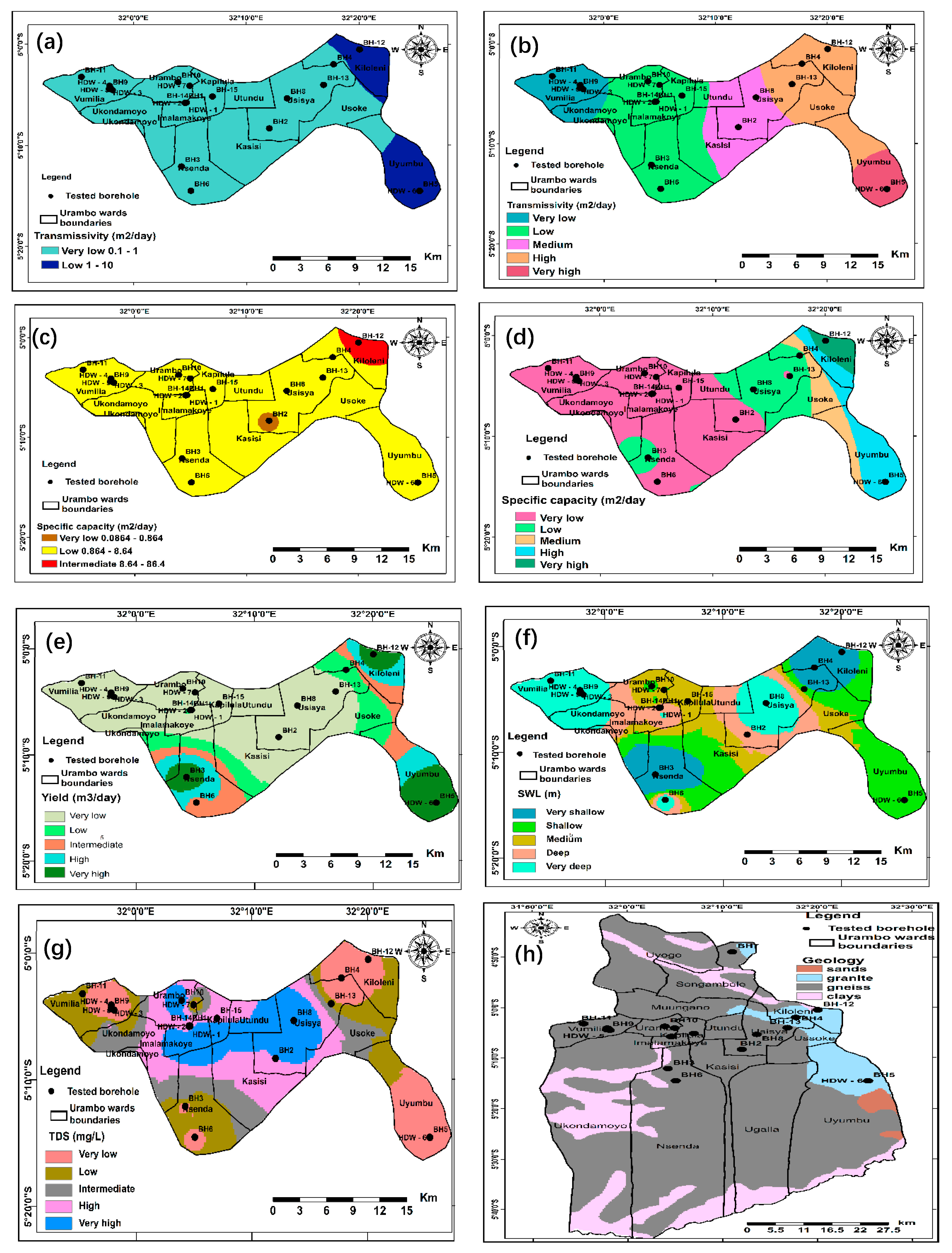
3.3. Development of Thematic Layers

The thematic layers were developed from transmissivity, specific capacity, yield, static water level, TDS, and geology maps (Figure 7).

3.3.1. Geology

The geological map of the study area was prepared using the geological map of the Tabora region as the base map. The thematic geologic map with an assigned weight of 31.03% (Table 8) (Figure 7h) indicates that the study area is underlain by four major rock types with different hydrogeological potential, namely sand, granite, gneiss, and clay. The sand area is considered to be a high groundwater potential zone, the granite area is considered to be a moderate groundwater potential zone, gneiss area is considered to be a low groundwater potential zone while the clay area is considered to be the least groundwater potential zone. The sand area is found in the eastern parts of the study area while granitic gneiss complex formation is dominant in the majority of the area. According to the rock characteristics, very high weight is assigned for sand, high weight is assigned for granite, moderate weight is assigned for gneiss, and low weight is assigned for clay. The regions with a significantly higher rating are considered to have good groundwater potential (Table 8).

3.3.2. Transmissivity

The transmissivity values for 15 boreholes, which were computed using Equation (1), ranged from 0.1 to 1.5 m2/day with a mean value of 0.7 m2/day (Table 7). These values were used to construct a transmissivity thematic map, which is classified based on both Kransy (Figure 7a) and research classification, which is based on the range of the acquired data (Figure 7b) with an assigned weight of 34.2% (Table 8).
Based on Kransy’s classification, the study area was categorized as an area with very low to low groundwater potential by [33] (Table 4) (Figure 7a) and according to this research classification, the area was categorized as very low (0.1–0.6 m2/day), low (0.6–1.0 m2/day), medium (1.0–1.6 m2/day), high (1.6–2.3 m2/day), and very high (2.3–3.0 m2/day), as illustrated in Figure 7b (Table 8). The well at Izimbili Village (BH No. 5) exhibited the highest transmissivity value of 1.5 m2/day with a transmissivity index value of 4.2 m2/day falling under a background anomaly that categorized the area as having potential for small withdrawal for local water supply (Table 4) while the lowest value of 0.1 m2/day was observed in Katanguru Village (BH-2) with a transmissivity index value of 3.02 m2/day falling under a negative anomaly which categorized the area as having potential for withdrawal for local water supply with limited consumption (Table 4).

3.3.3. Specific Capacity

The specific capacity values for 15 boreholes that were computed using Equation (2) ranged from 0.29 to 16.36 m2/day (mean = 3.7 m2/day) (Table 7). The generated Specific capacity map was also classified into both Kransy and research classifications with an assigned weight of 13.03% (Table 8). The specific capacity values computed ranges as presented in Table 7.
Based on Kransy’s classification [33], the study area was categorized as an area very low, low, and intermediate groundwater potential by [33] (Table 4) (Figure 7c). Based on this study, the area was categorized as area with very low (0.3–3.1 m2/day), low (3.1–5.7 m2/day), medium (5.7–9.0 m2/day), high (9.0–12.5 m2/day), and very high (12.5–16.4 m2/day) (Figure 7d).

3.3.4. Wells Yield

Well yields for 15 boreholes were determined through pumping tests and ranged from 10.8 to 108 m3/day with a mean value of 48.66 m3/day (Table 7). The generated well yield map was classified into five classes with an assigned weight of 12.39%: very high (77–108 m3/day), high (57–77 m3/day), intermediate (4–53 m3/day), low (31–43 m3/day), and very low (1–31 m3/day) (Figure 7e).

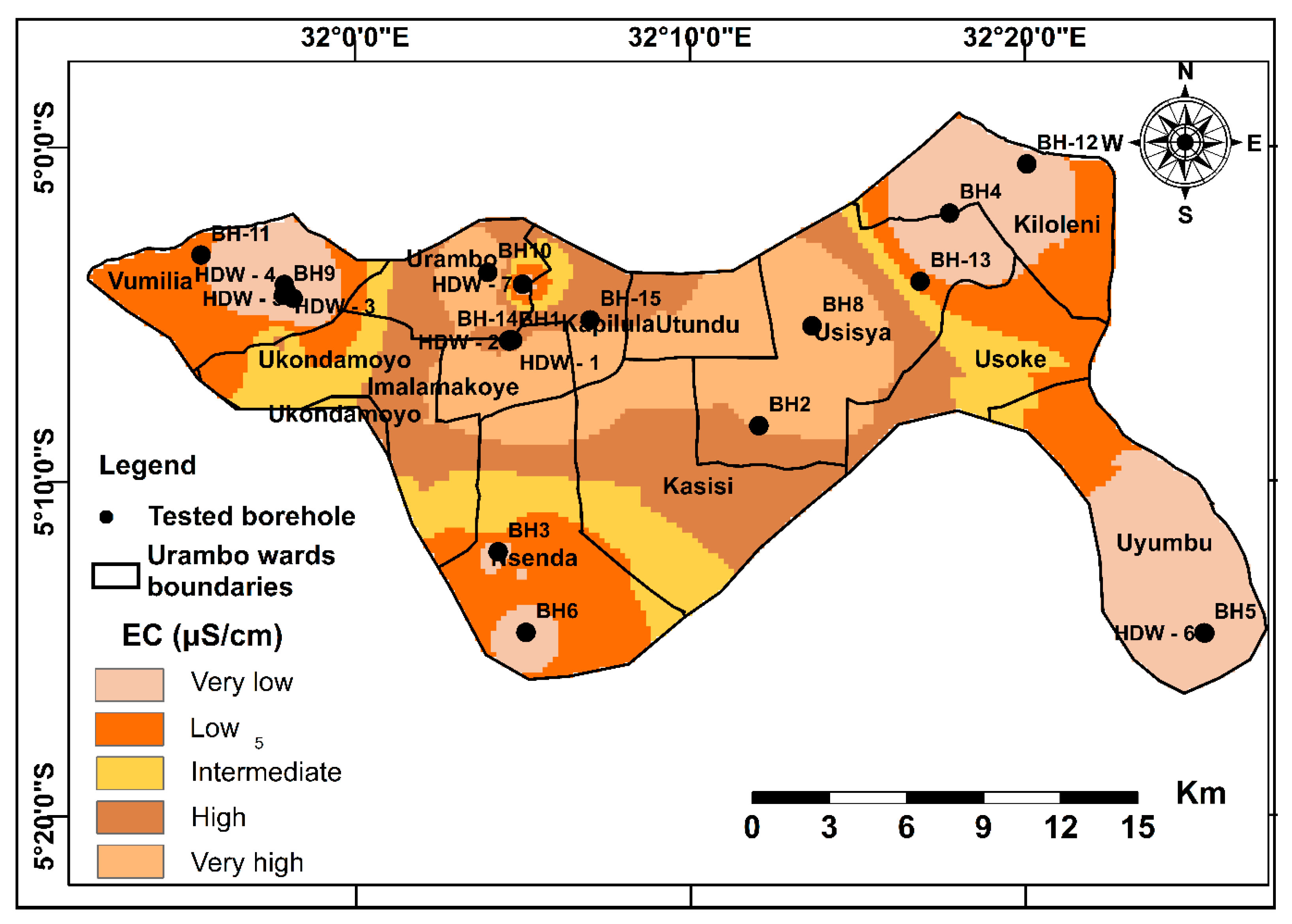
3.3.5. Total Dissolved Solids (TDS)

The total dissolved solids (TDS) ranged between 57 and 2445 mg/L (mean = 533 mg/L) (Table 6). The generated TDS map was classified into five classes with an assigned weight of 5.58%: very high (938.6–2423.4 mg/L), high (715.9–938.6 mg/L), intermediate (539.6–715.9 mg/L), low (344.7–539.6 mg/L), and very low (57.1–344.7 mg/L) (Figure 7g). The water with high TDS of 2445 mg/L (Table 6.) indicates that the water is highly mineralized. The desirable limit for TDS is 500 mg/L and the maximum limit is 1000 mg/L for water prescribed for drinking purpose [34,35]. Although the mean value shows that the TDS value is within the range recommended by the WHO [35], some boreholes were reported to exceed the permissible range.

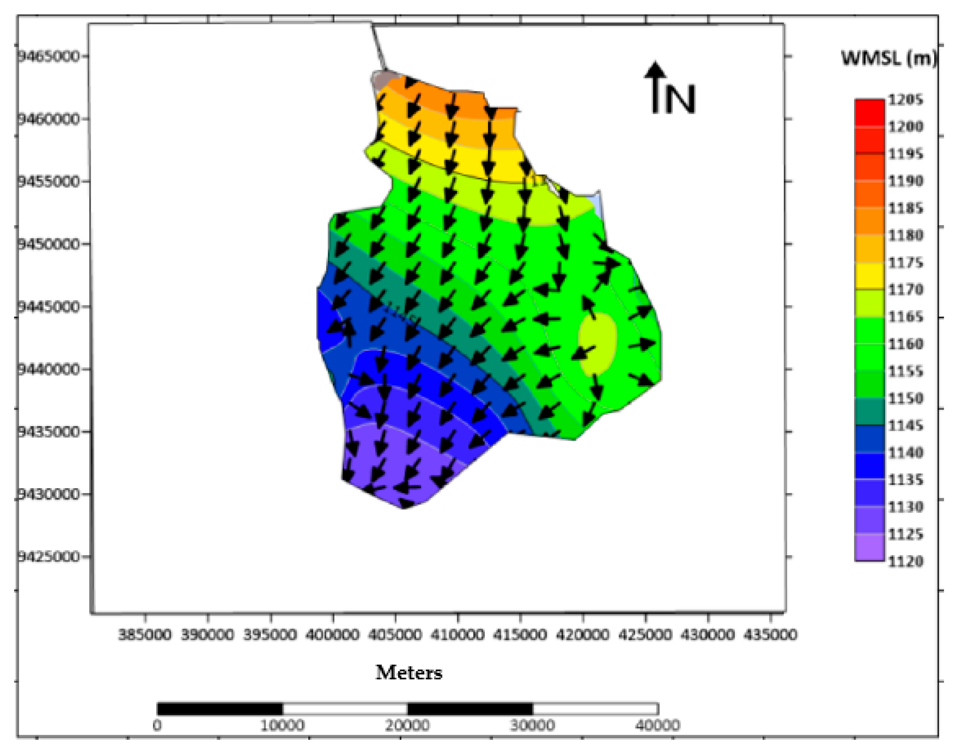
3.3.6. Static Water Level

The static water levels that were measured in 15 boreholes ranged between 0.60 and 7.97 m with a mean value of 3.5 m (Table 7). The generated static water level map was classified into five classes with an assigned weight of 3.79%: very shallow (0.6–2.2 m), shallow (2.2–3.2 m), medium (3.2–4.1 m), deep (4.1–5.1 m), and very deep (5.1–7.97 m) (Figure 7f) (Table 8).
For all thematic maps, the relevant weights were assigned to the six themes (static water level yield, total dissolved solids, transmissivity, specific capacity, and geology) based on the influence on groundwater development during the computation of AHP, as tabulated in Table 8. The value of CR obtained was 0.09 (Appendix C), implying that the criteria weight was based on a reasonable level of consistency. The factors and their classes are presented in Table 8.

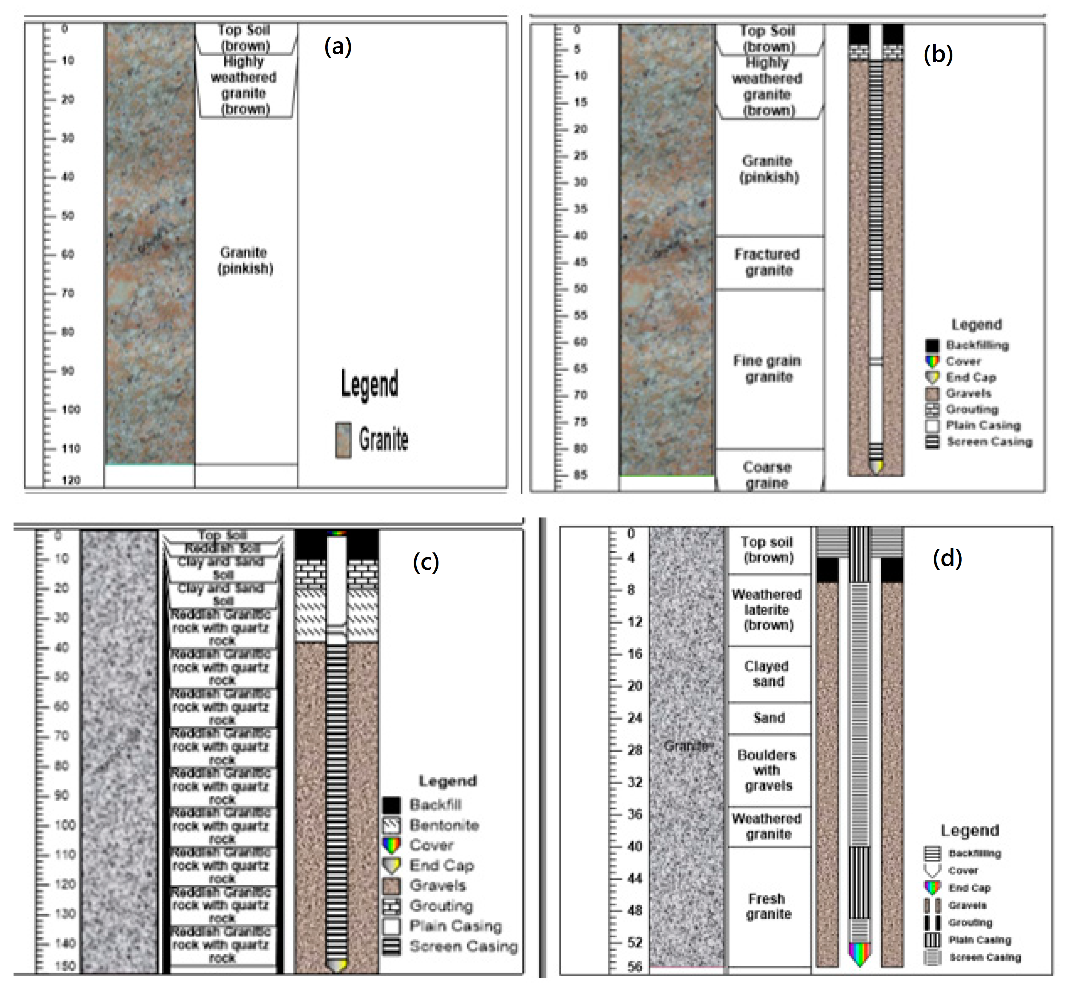
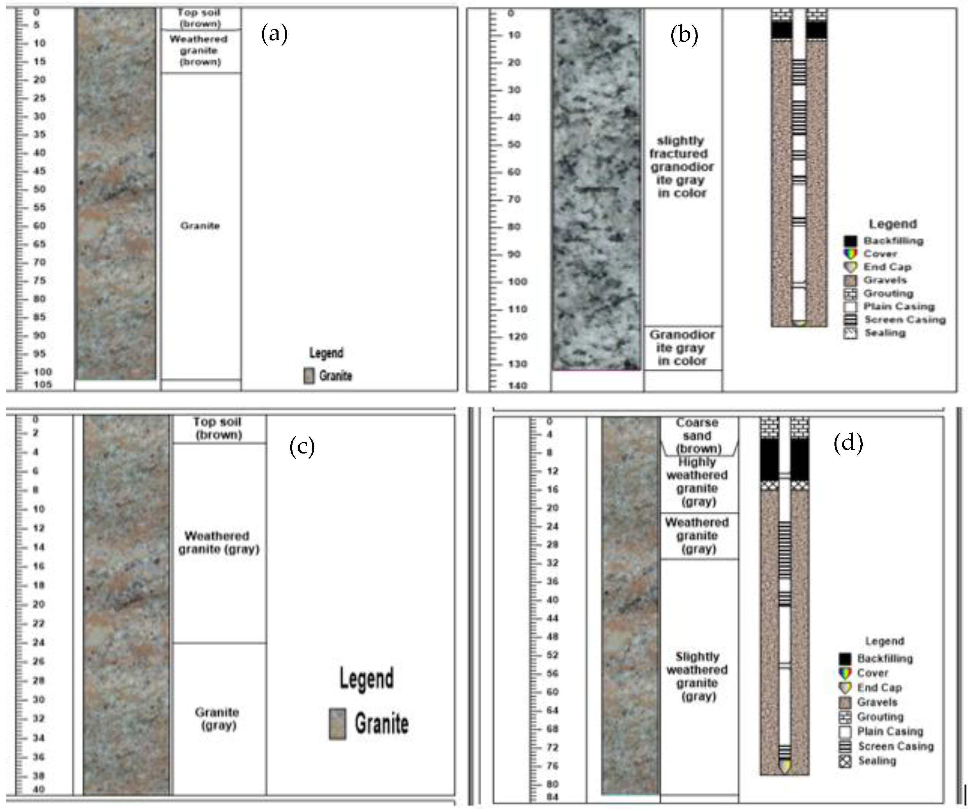
3.4. Lithological Logs

Lithological logs for eight boreholes are presented in Figure 8 and Appendix E. The results indicate that the upper part (0–8 m) is dominated by brown soils likely to be a mixture of organic matter and that the soils developed from the underling granitic gneiss formation. Granites extend to a depth of about 150 m and they are slightly weathered and fractured in some areas. Such weathered and fractured zones favor groundwater occurrence as the boreholes in such areas exhibit a high yield of 108 m3/d (Table 7) along with high transmissivity between 0.6 and 3 m2/d and a specific capacity between 3.09 and 16.36 m2/d. The boreholes located in fresh granitic and gneissic formations were found to be dry or to have a very low yield of 10.08 m3/d (Table 7).

4. Discussion

To evaluate groundwater potentiality in Urambo District, all datasets, which are pumping test data (15 boreholes), lithological logs (8 boreholes), and physico-chemical parameters in 28 wells, were integrated together to develop thematic layers for geology, specific capacity, transmissivity, total dissolved solids, static water level, and yield. Such information was further used to construct hydrogeological cross-sections and a groundwater potential index map as the basic tools for assessing groundwater occurrence and potentiality in the district.

4.1. Characterization of Groundwater

The extremely low electric conductivity (60 μS/cm, Table 6) that was recorded at BH-15 (Kapilula Village) is attributed to the low dissolution of ions from fresh granite, and the extremely high EC (3762 μS/cm, Table 6) that was recorded at BH-21 (Imalamakoye) is attributed to the high dissolution of gneiss formation which is relatively weak. BH-15 is located in a granitic zone, where groundwater is likely to be controlled by structures (Figure 2). BH-14, BH-22, BH-1, BH-19, BH-2, BH-8, and BH-9 were above the permissible limits of both WHO and TBS standards which are 120 and 1000 μS/cm, respectively [38]. The high EC values of the stated boreholes is basically due to integrated factors such as human activities, differential weathering, and the decomposition of organic matter, clay material, and salts resulting from evaporation–crystallization circles. Spatial variation of these values within the study area is shown in Figure 3. It is well indicated that the high EC values are generally in the central to northern part (Figure 3).
The highest turbidity values for boreholes BH-4, BH-5, BH-7, BH-13, HDW-I, HDW-2, HDW-3, HDW-4, and HDW-5 (Table 6) are attributed to their spatial locations. They are located in swampy areas, and therefore, the high turbidity is due to the high clay and organic matter content within the swamps, similar to [38].
The potential of hydrogen (PH) records in the study area is acidic. The acidity of the water in BH-14, 15, and 20 could be due to the geology or low water–sediment contact time relative to other areas. Such findings concur with the studies by [36,39].

4.2. Groundwater Occurrence

Groundwater occurrence is influenced by several factors that include but are not limited to topography, climate, geology, and material properties. The latter factor is subdivided into porosity and permeability, which are related to either primary or secondary porosity. Urambo District in particular is a basement crystalline that depends on secondary porosity as media for groundwater storage [23]. The secondary porosity results from chemical weathering, joining, shearing, and fracturing. Two main aquifer systems can be identified: the weathered zone aquifer system and the fractured zone aquifer system. The pumping test results as described earlier provided a good assessment of the case study data recorded.
The pumping test data were used to assess the aquifer characteristics largely through the boundary conditions and changes in drawdown. The time–drawdown curves shown in Figure 4, Figure 5 and Figure 6 reflect leaky aquifer conditions, barrier conditions, and recharge conditions, respectively. Both the first and last conditions are attributed to an increase in water storage, which leads to less drawdown at given times during the latter part of the test. Water may be added to the aquifer through leakage from the adjoining aquitards (semi-containing units) or recharge (e.g., to an unconfined aquifer from a surface water body or precipitation). However, the only difference between the two conditions is the degree of deflection; thus, the first has gentle deflection compared to the sharp deflection exhibited by the recharge condition [39]. The barrier condition in particular may be caused by low-permeability strata against the aquifer, causing the cone of depression to deepen instead of expanding laterally [40].
The highest specific capacity value of 16.36 m2/day at Kiloleni (BH-12) is associated with sands, gravels and clayey sand in shallow aquifers whereas the lowest specific capacity value of 0.29 m2/day at Katunguru (BH No. 2, Figure 7) is associated with slightly fresh gneiss with low permeability. Based on the specific capacity classification displayed in Table 4, about 87% of the tested boreholes do not have the capacity to establish communities’ water supply. BH-2 with a specific capacity value of 0.29 m2/day qualifies for the withdrawal of water for local water supply with limited consumption as specified by [33] while BH-12 with a specific capacity value of 16.36 m2/day qualifies for withdrawal for local water supply (small communities and plants).
In general, according to the classification magnitude of transmissivity and specific capacity [33], transmissivity values greater than 100 m2/day have high possibilities of groundwater potential [15]. In this study, the low drawdown, high transmissivity, and high specific capacity represent locations that are considered groundwater zones for development (Figure 7).
The variation in the distribution of transmissivity and specific capacity values in most pumping test locations in this study is almost the same, ranging from very low to low. This may be because of the presence of a thin layer of weathered rock and massive rock. This fact may be supported by borehole design; hence, the study area depends on shallow aquifer from alluvial deposits as observed in Kiloleni (BH-12) and Izimbili (BH-5).
According to [33] based on transmissivity magnitude, variation, and index, the study area falls under the groundwater supply potential of withdrawal for local water supply with limited consumption (Table 4), the hydrogeological environment is considerably heterogeneous because the standard deviation range is between 0.6–0.8 m2/day (Table 5), and 93% of the area is under background anomaly (Table 3) while 7% is under negative anomaly.
The well at Izimbili (BH-5) with the water supply with the highest yield value of 108 m3/day is located in depression area (Figure 7. The lithological borehole log (Figure 8 and Appendix E) indicates that it is composed of sediments varying from gravels and sands to clayey sand to a depth of 35 m. Thereafter, this is followed by granite to a depth of 55 m, which is the end of the hole. These data indicate that there is an unconfined shallow aquifer where groundwater is largely hosted in alluvial formation; these are likely to form shallow aquifers with a total depth of 55 m. The lowest yield value of 10.08 m3/day at Imalamakoye (BH-14) was located on a flat area with a total depth of 116 m. The lithological borehole log for this well revealed a fine sand, fine to medium sand sequence which is a derivative of granitic gneiss rocks (Figure 7h). The lithological logs of the drilled wells used for this study correlate positively and agree with the model produced by MacDonald [37]. However, 12 wells have yield values that vary between 0.12 and 0.72 L/s (10.08 and 62.4 m3/day). A previous study showed that most of the borehole yields in Precambrian crystalline basement rocks such as granitic gneiss range between 0.1–1 L/s (8.64–86.4 m3/day) [37], which agrees with findings of this study. Three boreholes however exhibited exceptionality by having yield values between 1 and 10 L/s due to coarse sand and gravel materials confined between the top clay layers hosted in alluvial deposits.
The high values of TDS in the study area as exhibited by BH-1, HDW-2, BH-9, BH-17, and BH-19 located in the town were probably due to residential runoff. Similarly, BH-2, BH-8, BH-18, and BH -21 located in swamps with clay materials were found to have high TDS values, probably due to the decomposition of organic and clay materials. These findings correspond to those of other researches [41,42]. High values of TDS in groundwater are generally not harmful to human beings [41], but high concentrations of these may affect people who are suffering from kidney and heart diseases [39].
The static water level of the study area is generally low, emphasizing that the hydraulic head is generally high across the study area as supported by other researchers [43]. This phenomenon can be ascribed to the thin overburden as well as favorable tropical climate conditions.
Geologically, the area is dominated by crystalline basement complex rocks (Figure 2) that form the basement aquifer, which was categorized into four major rock types with different hydrogeological potential, namely sand, granite, gneiss, and clay. The sand area is considered to be a high groundwater potential zone, the granite area is considered to be a moderate groundwater potential zone, the gneiss area is considered to be a low groundwater potential zone, and the clay area is considered to be the least groundwater potential zone. The areas with higher potential are associated with high permeability and relatively high transmissivity, while those with poor groundwater potential are associated with low permeability [44,45].

4.3. Groundwater Flow Direction

Groundwater flows from locations with more potential energy to areas with less potential energy. The black arrows in Figure 9 represent the direction of groundwater flow, which is deduced from the equipotential contours created using hydraulic heads. Groundwater flow direction and gradients are significantly influenced by the topography where the low land areas act as a major discharge area for both bedrock and buried sand and gravel aquifers [45]. The direction of groundwater flow in Urambo is both north–east and downward–southwest. A thick succession of granitic gneiss in the area appears to have some control over the gradient through this region as it exhibits very low hydraulic conductivity.

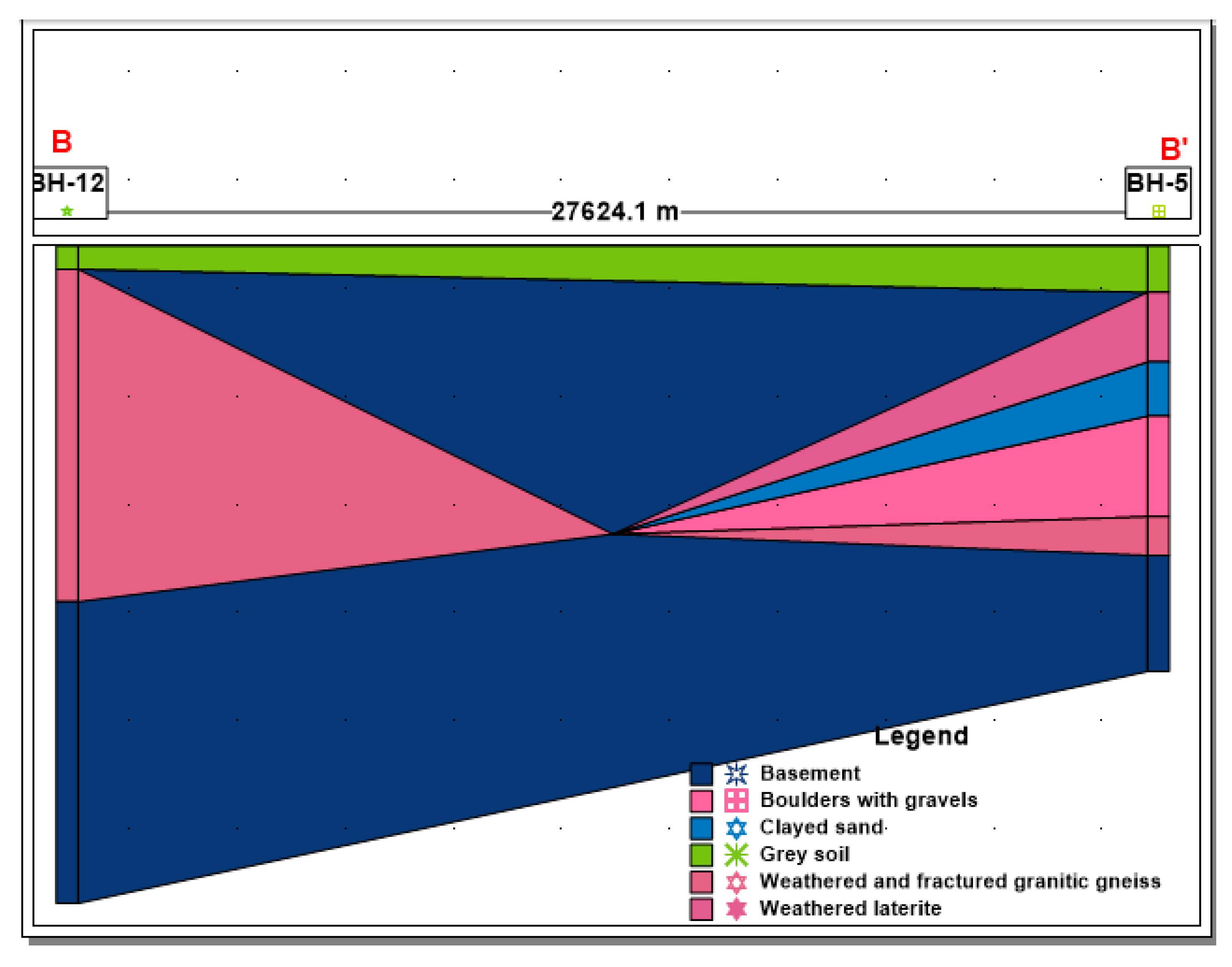
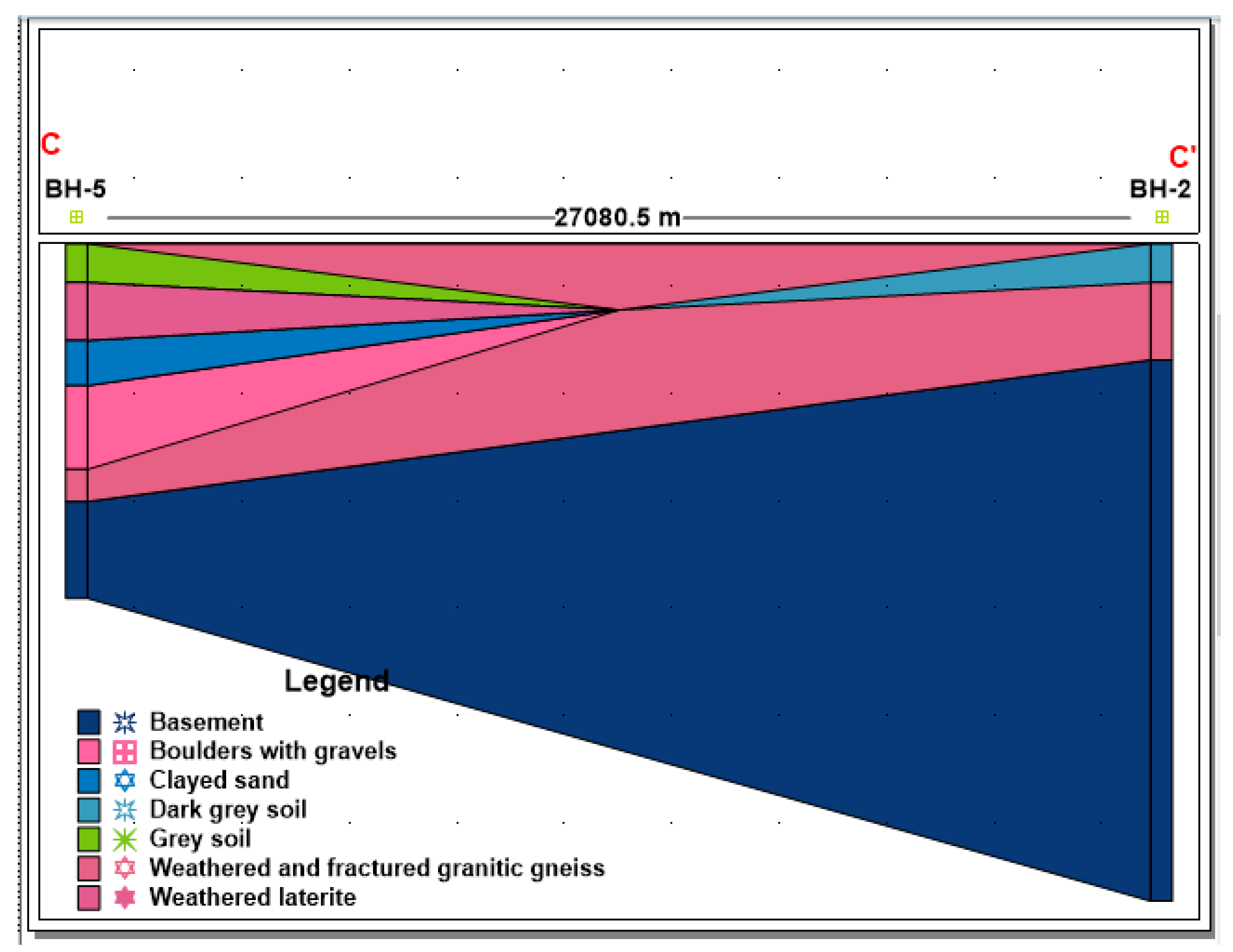
4.4. Hydrogeological Cross-Section

Hydrogeological cross-sections, as marked out in Figure 10, were developed to produce the horizontal and vertical extent of aquifers and aquitards commonly encountered in Urambo District. The eastern part of the study area has a more weathered and fractured formation than the western part. Likewise, the yield of the study area decreases towards the west.
The cross-section in Figure 11 and Figure A7 and Figure A8 in Appendix D illustrates the horizontal and vertical extent of aquifers and aquitards commonly encountered in Urambo. The cross-section identifies a surficial sand aquifer, quaternary buried sand and gravel aquifers, and two bedrock aquifers (weathered and fractured). The Quaternary buried sand and gravel aquifers are adequate for domestic wells, but variability in their thickness and extent can make them inadequate for large water supply wells that require higher pumping capacities. Most high-capacity wells (BH-5 and BH-12) with yields of 108 m3/d each (Figure 11) are constructed in Quaternary buried sand and gravel and weathered formation aquifers. The study area indicates that the yield increased from the western part to the eastern part due to an increase in the degree of weathering or fracturing and the thickness of the aquifer (Figure 11).

4.5. Groundwater Potential Index Map and Validation

A groundwater potential index map (GWPIM) was constructed by integrating maps of transmissivity, specific capacity, static water level, yield, TDS, and geology by preference with weights of 31%, 34.2%, 3.8%, 5.6%, 12.41%, and 13%, respectively, using the analytical hierarchy process (AHP) approach as discussed in Section 2.8. These parameters are direct indicators of groundwater potential in this study, which shows the spatial variation of groundwater potential across the study area. The groundwater potential index map (Figure 12) identified four distinct groundwater potential areas: least, low, moderate, and high. The majority of the study area (67%) was classified in the moderate groundwater potential zone, and 33% was classified in the high potential zone; high potential areas occupy parts of the eastern side of the study area as seen in Figure 12. The high groundwater potential area is attributed to the presence of alluvial deposits (sands) and weathered formations, which are located on depressions that make up some of the swamp area, with a high yield (108 m3/day) and high transmissivity values ranging from 1.5 to 3 m2/day. The presence of sand formations and high transmissivity values in this zone promises a high groundwater recharge rate, as supported by pumping test data from Izimbili Village (BH-5). The low groundwater potential zone in the western part was attributed to the presence of compacted geological formations which do not allow easy infiltration of rainwater and have low yield and transmissivity values. Generally, groundwater potential increases in Quaternary buried sand and gravel and weathered formation aquifers in the study area.
The developed GWPIM was validated using three boreholes (Figure 12) drilled in December 2022. The results are in agreement with the developed GWPI for the borehole at Kinhwa, which is drilled in a high potential zone (Figure 12) with an 88 m3/day yield and whose aquifers are controlled by Quaternary buried sand and gravel at a depth between 10 and 35 m. These findings are well supported by the pumping test results for BH-5 and BH-12, which are found in areas of high groundwater potential, and BH-9 and BH-11, which are found in areas of moderate groundwater potential. BH-5 and BH-12 exhibited the highest yield value of 108 m3/day and were located in high groundwater potential areas, while BH-9 and BH-11 had moderate yields of 33.48 and 32.76 m3/day, respectively, and were found to have moderate groundwater potential. Moreover, the other boreholes located in areas with moderate groundwater potential have low groundwater yields, for example, BH-2, BH-8, BH-14, and BH-15.

5. Conclusions

This study applied a customized indicator-based methodology for the evaluation of groundwater potential zones in a granitic gneiss aquifer formation in Urambo District. The use of integrated datasets for the evaluation of groundwater potentiality, especially pumping test data (SWL, yield, T, and SC), total dissolved solids (TDS), and geology, can adequately characterize groundwater potential zones in Urambo District with varying levels of influence. Higher weightages of 31% and 34.2% are suitable for geology and transmissivity, respectively. Similarly, moderate weights of 13%, and 12.4% for specific capacity and borehole yield, respectively, are proposed for such a granitic gneiss aquifer in Urambo District, whereas there are respective low weightages of 3.8%, and 5.6% for SWL and TDS. This study revealed that groundwater is controlled by Quaternary sediments and weathered to fractured granitic gneiss. Quaternary sediments, particularly sands and gravels, host the major shallow aquifers (<35 m) with relatively high transmissivity, specific capacity, and yield (1.5 m2/day, 16.36 m2/day, and 108 m3/day, respectively). The granitic gneiss in Urambo District is not strongly fractured/weathered and forms aquifers with a relatively low yield of about 10.08 m3/day. The hydrogeological cross-sections revealed that there is an increase in borehole yield as you move from the slightly weathered gneiss formation (12.7 m3/day) on the western side to the highly fractured and weathered granitic gneiss formation and alluvial (100.8 m3/day) on the eastern side. Such findings were validated using three boreholes, and the results are consistent with the developed groundwater potential index map.
Based on the analysis of the spatial variation of transmissivity magnitude and transmissivity variation, we classified the study area according to its groundwater supply potential, ranging from zones without groundwater supply prospects to withdrawals of lesser regional importance. The standard deviation of 0.7 m2/day in the transmissivity index identified the study area as a considerably heterogeneous hydrogeological environment. The overall implication of the data analysis in this research is that transmissivity index classification has been successfully applied to assess the groundwater resource potential of the study area. The results of the study are reliable and consistent with the geology of the study area. Aquifer characteristics are of crucial importance in groundwater prospecting.
Future studies should be planned to gather more pumping tests, drilling, and water quality parameters, which could increase the evaluation of groundwater potential using aquifer characteristics eligibility for use in Urambo district and other locations. Such findings are of great importance in groundwater development as the techniques applied can be extended to other areas in Tanzania as well as other countries that experience similar geological environments.

6. Recommendation

As it has been shown on the groundwater potentiality map that 67% of the study area is in low potential zones and 33% is in the moderate potential zone, borehole development should be centred in the demarcated moderate groundwater potential zone. Furthermore, due to the inadequate availability of groundwater data, this study recommends more groundwater studies in Urambo District.

Author Contributions

Conceptualization, A.R.Y.; methodology, A.R.Y., E.E.M., K.R.M. and I.C.M.; software, A.R.Y.; validation, A.R.Y., E.E.M., K.R.M. and I.C.M.; formal analysis, A.R.Y., E.E.M., K.R.M. and I.C.M.; investigation, A.R.Y.; resources, A.R.Y., E.E.M., K.R.M. and I.C.M.; data curation, A.R.Y., E.E.M., K.R.M. and I.C.M.; writing—original draft preparation, A.R.Y.; writing—review and editing, E.E.M., K.R.M., I.C.M. and A.R.Y.; visualization, A.R.Y., E.E.M., K.R.M. and I.C.M.; supervision, E.E.M., K.R.M. and I.C.M. All authors have read and agreed to the published version of the manuscript.

Funding

This research received no external funding.

Data Availability Statement

Not applicable.

Acknowledgments

The author wishes to acknowledge the Ministry of Water (MOW) through the Lake Tanganyika Basin Water Board (LTBWB) for giving permission to join the Degree of Hydrogeology and Water Resources Management. Also, special thanks are given to my supervisors and colleagues for the support and help given during the study. Last but not least, I want to express my gratitude to my family, including my parents, brothers, and sisters, for their prayers and support throughout my academic career. The assistance of several people in numerous ways was necessary to complete this effort. I want to genuinely thank them for everything.

Conflicts of Interest

The authors declare no conflict of interest.

Appendix A. Meteorological Data

Figure A1. Monthly average potential evapotranspiration and rainfall (2001–2021).
Earth 04 00042 g0a1
Figure A2. Monthly average maximum and minimum temperature.
Earth 04 00042 g0a2

Appendix B. Pumping Test Results as Interpreted by the Cooper and Jacob Method

Figure A3. Pumping test analysis result of the Kiloleni hand-dug well) where blue squares = Pumping Water Level (not used in interpretation), blue circles = Pumping Water Level (used in interpretation), red line = Best Fit Line while dotted line (u) = 0.05.
Earth 04 00042 g0a3
Figure A4. Pumping test analysis results of BH-2, BH-4, and BH-6 (recharge condition) where blue squares = Pumping Water Level (not used in interpretation), blue circles = Pumping Water Level (used in interpretation), red line = Best Fit Line while dotted line (u) = 0.05.
Earth 04 00042 g0a4
Figure A5. Pumping test analysis results of BH-10, BH-13, and BH-8 (barrier condition) where blue squares = Pumping Water Level (not used in interpretation), blue circles = Pumping Water Level (used in interpretation), red line = Best Fit Line while dotted line (u) = 0.05.
Earth 04 00042 g0a5

Appendix C. AHP Weighing Procedures and Results

Figure A6. AHP Weight Assignment during Groundwater Potential map Development.
Earth 04 00042 g0a6

Appendix D. Hydrogeological Cross-Section

Figure A7. Hydrogeological cross-section of the study area from B to B’.
Earth 04 00042 g0a7
Figure A8. Hydrogeological cross-section of the study area from C to C’.
Earth 04 00042 g0a8

Appendix E. Lithology and Well Design

Figure A9. The lithology and well design: (a) lithology of the dry borehole at Kiloleni, (b) lithology and well design of BH-12 at Kiloleni, (c) lithology and well design of BH-1, and (d) lithology and well design of BH-5.
Earth 04 00042 g0a9

References

  1. United Nations Children’s Fund (UNICEF). State of the World’s Hand Hygiene: A Global Call to Action to Make Hand Hygiene a Priority in Policy and Practice; UNICEF; WHO: New York, NY, USA, 2021; ISBN 9789280652901. [Google Scholar]
  2. Makoba, E.; Muzuka, A.N.N. Water quality and hydrogeochemical characteristics of groundwater around Mt. Meru, Northern Tanzania. Appl. Water Sci. 2019, 9, 120. [Google Scholar] [CrossRef]
  3. Mjemah, I.C.; van Camp, M.; Martens, K.; Walraevens, K. Groundwater exploitation and recharge rate estimation of a quaternary sand aquifer in Dar-es-Salaam area, Tanzania. Environ. Earth Sci. 2011, 63, 559–569. [Google Scholar] [CrossRef]
  4. UNICEF. Progress on Sanitation and Drinking Water; UNICEF: New York, NY, USA, 2015. [Google Scholar]
  5. Makoba, E.; Muzuka, A.N.N. Delineation of groundwater zones with contrasting quality in the fluorotic zone, around Mount Meru, northern Tanzania. Hydrol. Sci. J. 2021, 66, 322–346. [Google Scholar] [CrossRef]
  6. Braune, E.; Xu, Y. The Role of Ground Water in Sub-Saharan Africa. Groundwater 2010, 48, 229–238. [Google Scholar] [CrossRef]
  7. Elisante, E.; Muzuka, A.N.N. Occurrence of nitrate in Tanzanian groundwater aquifers: A review. Appl. Water Sci. 2017, 7, 71–87. [Google Scholar] [CrossRef]
  8. Kashaigili, J.J. Assessment of Groundwater Availability and Its Current and Potential Use and Impacts in Tanzania. 2010, pp. 1–67. Available online: https://www.suaire.sua.ac.tz/handle/123456789/1484 (accessed on 2 October 2023).
  9. Sadiki, H. Groundwater Management in Africa: The Case of Pangani Basin, Tanzania. In Proceedings of the 5th World Water Forum, Istanbul, Turkey, 20 March 2009. [Google Scholar]
  10. SMEC. Integrated Water Reources Management and Development Plans for Lake Tanganyika Basin Water Board; SMEC: Kigoma, Tanzanai, 2015. [Google Scholar]
  11. Davies, J.; Dochartaigh, B.Ó. Visit to Undertake Groundwater Development Studies in Tabora Region Tanzania (July–September 2000); British Geological Servey: Nottingham, UK, 2000. [Google Scholar]
  12. JICA. Project of Rural Water Supply in Tabora Region, Tanzania; Ministry of Water: Dodoma, Tanzania, 2011.
  13. Popoola, A.A.A.O.I.; Ogungbe, O.T.O.A.S.; Okediji, O.A.O.S.O. Assessment of groundwater potential and quality using geophysical and physicochemical methods in the basement terrain of Southwestern, Nigeria. Environ. Earth Sci. 2020, 79, 364. [Google Scholar] [CrossRef]
  14. Agbede, O.A.; Oyelakin, J.; Sciences, E.; Aiyelokun, O. Evaluation of Groundwater Potential through Aquifer Hydraulic Properties in Oyo State, Southwestern Basement Complex Nigeria. In Proceedings of the 2019 Civil Engineering Conference on Sustainable Construction for National Development, Ibada, Nigeria, 10–12 July 2019. [Google Scholar]
  15. Kumar, T.J.R.; Balasubramanian, A.; Kumar, R.S.; Dushiyanthan, C.; Thiruneelakandan, B.; Suresh, R.; Karthikeyan, K.; Davidraju, D. Assessment of groundwater potential based on aquifer properties of hard rock terrain in the Chittar—Uppodai watershed, Tamil Nadu, India. Appl. Water Sci. 2016, 6, 179–186. [Google Scholar] [CrossRef]
  16. Ugbaja, A.N.; William, G.A.; Ugbaja, U.A. Evaluation of Groundwater Potential Using Aquifer Characteristics on Parts of Boki Area, South—Eastern. J. Geol. Sci. 2021, 19, 93–104. [Google Scholar] [CrossRef]
  17. Gomo, M. On the practical application of the Cooper and Jacob distance-drawdown method to analyse aquifer-pumping test data. Groundw. Sustain. Dev. 2020, 11, 100478. [Google Scholar] [CrossRef]
  18. Mawlood, D.K.; Mustafa, J.S. Cooper-Jacob’s Method for Estimating of the Aquifer Parameters. Math. Model. Civ. Eng. 2016, 12, 9–20. [Google Scholar] [CrossRef]
  19. Council, U.D. Medium Term Rolling Strategic Plan for. 2018. Available online: https://urambodc.go.tz (accessed on 2 October 2023).
  20. Mwita, M.M. Shifting Cultivation, Wood Use and Deforestation Attributes of Tobacco Farming in Urambo District, Tanzania. Curr. Res. J. Soc. Sci. 2012, 4, 135–140. [Google Scholar]
  21. Quansah, A.D.; Dogbey, F.; Asilevi, P.J.; Boakye, P.; Darkwah, L.; Oduro-Kwarteng, S.; Sokama-Neuyam, Y.A.; Mensah, P. Assessment of solar radiation resource from the NASA-POWER reanalysis products for tropical climates in Ghana towards clean energy application. Sci. Rep. 2022, 12, 10684. [Google Scholar] [CrossRef] [PubMed]
  22. Cohen, K.; Finney, S.; Gibbard, P.; Fan, J.-X. International Chronostratigraphic Chart v2016/04. Int. Comm. Stratigr. 2013, 36, 199–204. [Google Scholar]
  23. Davies, J.; Dochartaigh, B.E.O. Low Permeability Rocks in Sub-Saharan Africa: Groundwater Development in the Tabora Region, Tanzania; British Geological Survey: Nottingham, UK, 2002; p. 76. [Google Scholar]
  24. Nakayama, H.; Yamasaki, Y.; Ohashi, K.; Nakaya, S. Simple method for estimating well yield potential through geostatistical approach in fractured crystalline rock formations. J. Hydrol. 2021, 597, 125719. [Google Scholar] [CrossRef]
  25. Gleeson, T.; Manning, A.H. Regional groundwater flow in mountainous terrain: Three-dimensional simulations of topographic and hydrogeologic controls. Water Resour. Res. 2008, 44, W10403. [Google Scholar] [CrossRef]
  26. Ige, O.O.; Obasaju, D.O.; Baiyegunhi, C.; Ogunsanwo, O.; Baiyegunhi, T.L. Evaluation of aquifer hydraulic characteristics using geoelectrical sounding, pumping and laboratory tests: A case study of Lokoja and Patti Formations, Southern Bida Basin, Nigeria. Open Geosci. 2018, 10, 807–820. [Google Scholar] [CrossRef]
  27. Chikira, I.; Van Camp, M.; Walraevens, K. Groundwater exploitation and hydraulic parameter estimation for a Quaternary aquifer in Dar-es-Salaam Tanzania. J. African Earth Sci. 2009, 55, 134–146. [Google Scholar] [CrossRef]
  28. Kale, V.; Quality, W.; Roosevelt, L.; Manual, S. Water quality sampling using in situ water quality instruments 1 Purpose and scope. Int. Adv. Res. J. Sci. Eng. Technol. ISO 2008, 3297, 1–11. [Google Scholar]
  29. Halford, K.J.; Weight, W.D.; Schreiber, R.P. Interpretation of Transmissivity Estimates from Single-Well Pumping Aquifer Tests. Groundwater 2006, 44, 467–471. [Google Scholar] [CrossRef]
  30. Nwankwoala, H.O. Application of Aquifer Parameters in Evaluating Groundwater Potential of Logo Area, Benue State, Nigeria. Int. J. Environ. Sci. Nat. Resour. 2018, 11, 1–8. [Google Scholar] [CrossRef]
  31. Kennedy, O.A. Hydrogeophysical studies for the determination of aquifer hydraulic characteristics and evaluation of groundwater potential: A case study of some selected parts of Imo River Basin, South Eastern Niger. Int. J. Sci. Res. Publ. 2020, 10, 738–755. [Google Scholar] [CrossRef]
  32. Hasan, M.; Shang, Y.; Akhter, G.; Jin, W. Geophysical Assessment of Groundwater Potential: A Case Study from Mian Channu Area, Pakistan. Groundwater 2018, 56, 783–796. [Google Scholar] [CrossRef] [PubMed]
  33. Krásný, J. Classification of Transmissivity Magnitude and Variation. Groundwater 1993, 31, 230–236. [Google Scholar] [CrossRef]
  34. Sapkota, S.; Prasad, V.; Bhattarai, U.; Panday, S. Groundwater potential assessment using an integrated AHP-driven geospatial and field exploration approach applied to a hard-rock aquifer Himalayan watershed. J. Hydrol. Reg. Stud. 2021, 37, 100914. [Google Scholar] [CrossRef]
  35. WHO. Guidelines for Drinking-Water Quality; WHO: Geneva, Switzerland, 2022; Volume 33, ISBN 9789240045064. [Google Scholar]
  36. Oberlin, A.S.; Ntoga, S. Quality Assessment of Drinking Water in Sumve Kwimba District. Am. J. Eng. Res. 2018, 7, 26–34. [Google Scholar]
  37. MacDonald, A.; Bonsor, H.; Calow, R.; Taylor, R.; Lapworth, D.; Maurice, L.; Tucker, J.; Dochartaigh, B. Groundwater Resilience to Climate Change in Africa; British Geological Survey Open Report: OR/11/031; British Geological Survey: Nottingham, UK, 2011; pp. 1–24. Available online: http://nora.nerc.ac.uk/id/eprint/15772/1/OR11031.pdf (accessed on 2 October 2023).
  38. Herschy, R.W. Water Quality for Drinking: WHO guidelines. In Encyclopedia of Lakes and Reservoirs; Springer: Dordrecht, The Netherlands, 2012; pp. 876–883. [Google Scholar] [CrossRef]
  39. Meride, Y.; Ayenew, B. Drinking water quality assessment and its effects on residents health in Wondo genet campus, Ethiopia. Environ. Syst. Res. 2016, 5, 1. [Google Scholar] [CrossRef]
  40. Lehigh University. Total Dissolved Solids. EnviroSci Inquiry. Available online: https://ei.lehigh.edu/envirosci/watershed/wq/wqbackground/tdsbg.html#:~:text=2.-,Concentration%20of%20total%20dissolved%20solids%20that%20are%20too%20high%20or,an%20increase%20in%20water%20temperature (accessed on 2 October 2023).
  41. Testing for Total Dissolved Solids. Available online: www.epa.gov/safewater/consumer/pdf/ (accessed on 2 October 2023).
  42. Adjovu, G.E.; Stephen, H.; James, D.; Ahmad, S. Measurement of Total Dissolved Solids and Total Suspended Solids in Water Systems: A Review of the Issues, Conventional, and Remote Sensing Techniques. Remote Sens. 2023, 15, 3534. [Google Scholar] [CrossRef]
  43. Acharya, T.; Prasad, R. Hydrodynamic Study of Weathered Zone of Hardrock Aquifers Using Dugwell Data. Nat. Resour. Res. 2014, 23, 331–340. [Google Scholar] [CrossRef]
  44. Kubingwa, J.N.; Makoba, E.E.; Mussa, K.R. Integrated Geospatial and Geophysical Approaches for Mapping Groundwater Potential in the Semi-Arid Bukombe District, Tanzania. Earth 2023, 4, 241–265. [Google Scholar] [CrossRef]
  45. Nayak, S.; Mukhopadhyay, B.P.; Mitra, A.K.; Chakraborty, R. Structural control on the occurrence of groundwater in granite gneissic terrain, Purulia, West Bengal. Arab. J. Geosci. 2020, 13, 955. [Google Scholar] [CrossRef]
Figure 1. Location and accessibility map of the study area.
Earth 04 00042 g001
Figure 2. Geological map of the study area with both the dry boreholes and the productive boreholes that were involved in the pumping test. (Modified from JICA (2011)).
Earth 04 00042 g002
Figure 3. A map of the spatial distribution of electrical conductivity in the study area.
Earth 04 00042 g003
Figure 4. Pumping test analysis result of the Itebulanda borehole (BH No 3) in leaky aquifer conditions where blue squares = Pumping Water Level (not used in interpretation), blue circles = Pumping Water Level (used in interpretation), red line = Best Fit Line while dotted line (u) = 0.05.
Earth 04 00042 g004
Figure 5. Pumping test analysis result of the Kiloleni borehole (BH No 12) in barrier conditions where blue squares = Pumping Water Level (not used in interpretation), blue circles = Pumping Water Level (used in interpretation), red line = Best Fit Line while dotted line (u) = 0.05.
Earth 04 00042 g005
Figure 6. Pumping test analysis result of Kichangani (Ukwanga) in recharge conditions where blue squares = Pumping Water Level (not used in interpretation), blue circles = Pumping Water Level (used in interpretation), red line = Best Fit Line while dotted line (u) = 0.05.
Earth 04 00042 g006
Figure 7. The thematic maps of the study area: (a,b) the transmissivity maps of which (a) refer to Kransy’s classification and (b) refers to this study classification, (c,d) specific capacity maps where (c) refers to Kransy’s classification and (d) refers to this study classification, (e) well yield map, (f) static water level map, (g) TDS map, and (h) geological map.
Earth 04 00042 g007
Figure 8. The lithology and well design: (a) lithology of the dry borehole at Imalamakoye, (b) lithology and well design of BH-14 at Imalamakoye, (c) lithology of the dry borehole at Kapilula, and (d) lithology and well design of BH-15 at Kapilula.
Earth 04 00042 g008
Figure 9. Equipotential lines and groundwater flow direction in Urambo District.
Earth 04 00042 g009
Figure 10. Spatial map showing boreholes involved in hydrogeological cross-sections: CC’ line from BH- 2 to BH-5, AA’ line from BH-2 to BH-12, and BB’ line from BH-5 to BH-12.
Earth 04 00042 g010
Figure 11. Hydrogeological cross-section of the study area from A to A’; the location of each borehole is shown in Figure 10 (not to scale).
Earth 04 00042 g011
Figure 12. Groundwater potential index map (GWPIM) of the study area.
Earth 04 00042 g012
Table 1. Mean monthly climate parameters of the area for the duration of 20 years.
MonthPET (mm/Month)PPT (mm/Month)TMax
(°C)
TMin
(°C)
TMean
(°C)
Aridity IndexAridity Status
January2121563715260.74Humid
February2131413714250.66Humid
March2101423615260.68Humid
April1981133515250.57Dry sub-humid
May200253412230.12Arid
June20373411220.03Hyper-arid
July20523410220.01Hyper-arid
August21443612240.02Hyper-arid
September226113814260.05Hyper-arid
October223393816270.17Arid
November2181593816270.73Humid
December2041993514250.97Hyper-humid
Total2525997
Average210833614250.40SEMI-ARID
Source: https://power.larc.nasa.gov/data-access-viewer/, accessed on 15 September 2023 (Power Access Climate Data).
Table 2. Aridity index values and climate classes.
S/NAridity Index (AI) Values
(Thornthwaite Method)
Climate Classification
1AI < 0.05Hyper-arid
20.05 < AI < 0.2Arid
30.2 < AI < 0.5Semi-arid
40.5 < AI < 0.65Dry sub-humid
50.65 < AI < 0.75Humid
6>0.75Hyper-humid
Source: United Nations Environment Programme (www.undep.org, accessed on 15 September 2023).
Table 3. Analysis of transmissivity values based on transmissivity index (Y) classification.
ClassificationDescriptionRange of ‘Y’ of Studied Area
Negative extreme anomaliesLess than [mean—(2 * standard deviation)]<[mean—(2 * standard deviation)]
Negative anomaliesBetween (mean—standard deviation) and [mean—(2 * standard deviation)]Between (mean—standard deviation) and [mean—(2 * standard deviation)]
Background anomaliesBetween (mean—standard deviation) and (mean + standard deviation)Between (mean—standard deviation) and (mean + standard deviation)
Positive anomaliesBetween (mean + standard deviation) and mean + (2 * standard deviationBetween (mean + standard deviation) and mean + (2 * standard deviation
Positive extreme anomaliesGreater than [mean + (2 * standard deviation)]>[mean + (2 * standard deviation)]
Table 4. Classification of transmissivity magnitude and specific capacity based on Kransy’s classification.
Magnitude of Transmissivity (m2/Day)ClassStatusSpecific Capacity (m2/Day)Groundwater Supply Potential
>1000IVery High>864Withdrawals of great regional importance
100–1000IIHigh86.4–864Withdrawals of less regional importance
10–100IIIIntermediate8.64–86.4Withdrawal for local water supply (small communities and plants)
1–10IVLow8.64-0.864Small withdrawal for local water supply (private consumption)
0.1–1VVery low0.0864–0.864Withdrawal for local water supply with limited consumption
<0.1VIImperceptible<0.0864Sources of local water supply are limited
Table 5. Classification of transmissivity variation based on Kransy’s classification.
Standard Deviation of Transmissivity Index (Y)Class of Transmissivity VariationStatus of Transmissivity VariationHydrogeological Environment
<0.2aInsignificantHomogenous
0.2–0.4bSmallSlightly heterogeneous
0.4–0.6cModerateFairly heterogenous
0.6–0.8dLargeConsiderably heterogenous
0.8–1.0eVery largeVery heterogenous
>1.0fExtremely largeExtremely heterogenous
Table 6. Physicochemical parameters for 28 sampled wells in Urambo District.
WellLocationWater SourceWater Quality Parameter
Temp.pHECTDSTurbidity
(°C) (µS/cm)(mg/L)(NTU)
BH-1MasakiBH26.97.67139390214.8
BH-2KatunguruBH30.97.74176511420
BH-3ItebulandaBH24.88.23562300
BH-4KalembelaBH25.78.113285176
BH-5IzimbiliBH27.68.5313285218
BH-6Utenge (Mkola)BH27.98.044392857.3
BH-7Kichangani (Ukwanga)BH297.8885746.1
BH-8UsisyaBH25.27.6176511420
BH-9MotomotoBH26.18.1102266219.9
BH-10Extended P/SchoolBH28.97.744012620
BH-13SipunguBH257.159028630
BH-12KiloleniBH 7.2144028615
BH-14ImalamakoyeBH 6.662.9 2.1
BH-15KapilulaBH 6.460.4 3
BH-16Itebulanda P/SchoolBH26.38.042471620
BH-17Itebulanda DispensaryBH24.97.791759417.5
BH-18Nsenda KanogeBH26.37.649726277.3
HDW -1MasakiHDW25.67.7491319150
HDW -2MasakiHDW26.37.485555339.2
BH-19BlockBH28.87.72155293110.3
HDW-3MotomotoHDW26.37.829419127.5
HDW-4MotomotoHDW27.17.7326116926.1
HDW-5MotomotoHDW27.77.5822814851.9
HDW-6IzimbiliHDW27833121323.1
HDW-7MwengeHDW28.97.744012620
BH-20UsokeBH27.16.8352330217
BH-21Imalamakoye W/SupplyBH277.79376224458.3
BH-22Ukimbizini W/SupplyBH27.67.4209213590.5
HDW-8KiloleniHDW 7.2395.561.89
Max. 30.98.537622445218
Min. 24.86.460570
Stdev 1.50.581553354
Median 277.743928615
Mean 277.677052733
Mean ± STD 27 ± 1.57.6 ± 0.5770 ± 815527 ± 53333 ± 54
WHO (STD) Nm6.5–8.51207505
TBS (STD) Nm6.5–9.210005005–25
STD = standard deviation, TBS = Tanzania Bureau Standards, Max = maximum, Min = minimum, EC = electric conductivity, TDS = total dissolved solids, Temp. = temperature, and HDW = hand-dug well.
Table 7. Summary of pumping test results.
BHSWL (m)Depth (m)Yield (m3/d)Drawdown (m)Sc (m2/d)T (m2/d)Y (m2/d)Range of ‘Y’
BH-13.5315061.316.663.680.73.873.12–4.52
BH-23.410012.744.270.290.13.022.42–3.12
BH-31.5610210834.973.090.63.803.12–4.52
BH-40.69544.4538.461.160.23.323.12–4.52
BH-54.285510812.948.351.54.203.12–4.52
BH-66.3413062.427.42.280.43.633.12–4.52
BH-71.062752.87.387.151.34.143.12–4.52
BH-87.9750244.475.3714.023.12–4.52
BH-92.18333.4817.251.940.43.633.12–4.52
BH-107.16431.6821.781.450.33.503.12–4.52
BH-112.29032.7636.90.890.23.323.12–4.52
BH-121.6851086.616.3634.53.12–4.52
BH-132.3515028.817.441.650.33.53.12–4.52
BH-141.8913210.0810.270.980.183.283.12–4.52
BH-156.0377.8811.528.391.370.223.373.12–4.52
Mean 20.35 0.693.82
Standard Deviation 0.70
BH = borehole, SWL = static water level, Sc = specific capacity, T = transmissivity, Y = transmissivity index, and d = day.
Table 8. The percentage of assigned weight for the thematic layers.
ThemeWeight (%)ClassClass DescriptionRank
SWL3.7910.60–2.239
22.23–3.248
33.24–4.057
44.05–5.116
55.11–7.975
Yield12.39111.6–30.85
230.8–42.96
342.9–57.37
457.3–77.08
577.0–108.09
TDS5.58157.05–344.715
2344.71–539.596
3539.59–715.917
4715.91–938.628
5938.62–2423.389
Transmissivity34.1810.1–0.585
20.58–1.046
31.04–1.647
41.64–2.298
52.29–3.009
SC13.0310.29–3.065
23.06–5.716
35.71–8.997
48.99–12.528
512.52–16.369
Geology31.031Sands9
2Weathered/fractured gneiss7
3Weathered/fractured granite8
4Clay2
Disclaimer/Publisher’s Note: The statements, opinions and data contained in all publications are solely those of the individual author(s) and contributor(s) and not of MDPI and/or the editor(s). MDPI and/or the editor(s) disclaim responsibility for any injury to people or property resulting from any ideas, methods, instructions or products referred to in the content.

