Article

Exploratory Analysis of the Interactions Between Territorial Development Patterns and Electricity Demand in Ecuador’s Coastal Region

1
Faculty of Engineering Sciences, Technical State University of Quevedo, Quevedo 120301, Ecuador
2
Department of Electrical Engineering, Universidad de Jaén, 23700 Jaén, Spain
3
Departamento de Ciencias de la Energía y Mecánica, Universidad de las Fuerzas Armadas ESPE, Sangolquí 171103, Ecuador
*
Author to whom correspondence should be addressed.
Electricity 2026, 7(3), 79; https://doi.org/10.3390/electricity7030079
Submission received: 15 April 2026 / Revised: 4 June 2026 / Accepted: 5 June 2026 / Published: 1 August 2026
(This article belongs to the Special Issue Feature Papers to Celebrate the First Impact Factor of Electricity)

Abstract

This study proposes a reproducible exploratory framework to link long-term territorial development with electricity demand in data-scarce contexts, and applies it to Ecuador’s Costa region. The pipeline combines three commonly available input streams: periodic census microdata, an official demand series, and macroeconomic aggregates. Socioeconomic heterogeneity across five non-uniform census rounds (1974, 1982, 1990, 2001, 2010) is summarized through Principal Component Analysis (PCA), and territorial indicators are projected to the demand horizon using a univariate linear trend. Eleven regression specifications are compared on a log-transformed demand variable, and a rolling-origin backtesting scheme plus a 2020–2024 holdout are used for validation. The selected Trend OLS log model attains R 2 = 0.551 and MAPE = 6.08%, and projects a regional demand of approximately 7055 MW by 2050, equivalent to a compound annual growth rate of 3.46%. Beyond the Ecuadorian case, the results show that transparent, low-data pipelines based on harmonized census information, macroeconomic drivers and simple regression models can provide defensible medium- and long-term demand signals for planners in other emerging economies with limited high-frequency data.

1. Introduction

In developing countries, electricity demand does not respond solely to technical or climatic factors: it is equally shaped by where people live, how the local economy is structured, and by the unequal distribution of infrastructure access [1,2]. This territorial perspective matters because models that ignore the spatial distribution of consumption tend to underestimate imbalances that are later costly to correct. Anticipating future supply requirements therefore demands integrating socioeconomic and spatial dimensions into the analysis, not merely aggregated load data.
Ecuador’s Costa region comprising Guayas, Manabí, El Oro, Esmeraldas, Santa Elena, Santo Domingo de los Tsáchilas, and Los Ríos, accounts for approximately 53% of the national population and generates more than 46% of GDP [3,4]. Its warm-humid climate (average temperature 25–28 °C, relative humidity above 70%) produces consumption profiles with high shares of air conditioning and agro-industrial processing [3]. Analysis is further complicated by the region’s internal heterogeneity: while Guayas concentrates industrial and commercial activity, Esmeraldas and Los Ríos exhibit higher poverty rates and lower electricity coverage, generating divergent demand structures that aggregate national analyses fail to capture.
The 2023–2024 energy crisis revealed the extent to which these territorial asymmetries carry real operational consequences. The dependence of the National Interconnected System (SNI) on hydroelectric generation, which accounted for 67.4% of total production in 2024, made it critically vulnerable to hydrological variability; a prolonged drought resulted in blackouts of up to 14 h per day [5]. The problem was therefore not solely one of installed capacity: it was also one of mismatch between the spatial distribution of generation and the territorial patterns of demand, a type of structural gap that conventional energy planning approaches frequently underestimate.
The literature on tropical coastal regions documents that temperature accounts for between 40% and 60% of consumption variability ( R 2 = 0.40 0.60 ), with typical increases of 2–4% per degree Celsius attributable primarily to air conditioning use; Pearson coefficients reported range from 0.65 to 0.85 [6,7,8]. Relative humidity shows moderate association with consumption ( r = 0.35 0.55 ) [4,9], while the effects of phenomena such as El Niño on demand in the Costa region have not been rigorously quantified [10,11,12]. In the socioeconomic dimension, income elasticities lie between 0.6 and 1.2 in developing economies [13], and residential price elasticities range from 0.2 to 0.5 in the short run and from 0.4 to 0.8 in the long run [2,14]. Territorial configuration variables such as population density, urbanization, and household size show significant positive correlations with consumption ( r = 0.55 0.75 ), while poverty and limited access to basic services are negatively associated [3,4]. At the temporal level, monthly seasonality accounts for between 15% and 25% of variability in tropical zones, with afternoon peaks that can exceed base demand by up to 40% [15]. Multivariate models integrating these three dimensions achieve explanatory levels of R 2 = 0.75 0.90 [2], confirming that no single category of predictors is sufficient on its own.
Machine learning tools have considerably expanded the possibilities for territorial analysis. LSTM networks achieve prediction errors (MAPE) of 1.5–3.5%, compared to 4–7% for ARIMA models [16,17]; Random Forest and XGBoost reach MAPE of 2–4% with R 2 > 0.95 [18]; and hybrid models with time series decomposition yield additional precision gains of 15–25% [19]. However, the transfer of these methods to data-scarce economies faces important constraints, as consumption patterns [20,21], technological access, and energy infrastructure differ substantially from the contexts in which these algorithms were originally developed [22,23]. In Ecuador, recent studies illustrate both the potential and the limitations of this field: Chicaiza Yugcha et al. [12] obtained a MAPE of 3.2% and R 2 of 0.94 at the subnational scale using multiple linear regression; Carrillo Calderón et al. [3] compared Random Forest and XGBoost in Chimborazo with accuracies above 92%; Moya et al. [24] identified seven determinants of residential consumption at 1 km2 resolution, including population density, GDP, and HDI; Araujo-Vizuete et al. [25] documented significant differences between Quito and Guayaquil associated with income and technological access; Icaza-Alvarado et al. [26] reported temperature-demand correlations between R 2 = 0.70 and R 2 = 0.85 with income elasticities of 0.8 to 1.1; and Naranjo-Silva et al. [23], using the LEAP model, documented the 2023–2024 crisis and estimated losses of approximately USD 2 billion. Despite these advances, disaggregated analysis of the Costa region remains limited.
The available evidence taken together indicates that climatic variables particularly temperature and humidity significantly influence electricity demand in tropical regions. Socioeconomic and demographic factors such as income, urbanization, population density, and access to infrastructure also strengthen the explanatory power of models when integrated in multivariate approaches. The literature further shows that machine learning methods and hybrid models generally outperform traditional statistical approaches in well-resourced settings. In Ecuador, the reliability problems of the electricity system are closely linked to the territorial distribution of generation and demand. Yet knowledge gaps persist for the Costa region, owing to the scarcity of comprehensive studies and limited availability of consumer-level data.
The transferability of advanced machine-learning methods to data-scarce economies is constrained both by the size of the available series and by the absence of high-frequency socioeconomic information. The literature on long-horizon demand forecasting in this regime is mature but fragmented: Bhattacharyya and Timilsina [27] systematically review top-down and bottom-up energy-planning frameworks for low-data economies; Suganthi and Samuel [28] document the persistent advantage of parsimonious econometric specifications when fewer than thirty annual observations are available; Hyndman and Athanasopoulos [29] formalize the rolling-origin validation protocol adopted here; and Debnath and Mourshed [30] map the trade-off between data requirements and predictive accuracy across a representative sample of emerging-economy applications. These contributions provide the methodological backdrop against which the present framework should be read, and they consistently support the design choice—articulated in Section 2—of a transparent, low-parameter framework complemented by rigorous out-of-sample validation.
Against this background, this study analyzes the relationship between territorial development patterns and electricity demand in Ecuador’s Costa region. Its contribution lies in jointly integrating territorial, socioeconomic, and macroeconomic factors within a transparent, reproducible framework to generate evidence useful for more robust, equitable, and resilient energy planning.
Although several studies have addressed electricity demand modeling in Latin America, few frameworks are explicitly designed for contexts in which high-frequency socioeconomic information is unavailable and where the only territorial signal comes from widely spaced national censuses. In Ecuador, for example, the national population and housing censuses used in this work correspond to 1974, 1982, 1990, 2001 and 2010, which defines a non-uniform temporal grid that does not align naturally with the annual demand series. This mismatch between slow-moving territorial drivers and annual electrical consumption has been largely overlooked in previous regional studies [5,23,26].
The present work contributes to this gap by proposing an exploratory, reproducible pipeline that can be read at two levels. At a general level, it provides a methodological template for linking heterogeneous territorial indicators with long-term demand in any region where census microdata, an official demand series and macroeconomic aggregates are available. At an applied level, it instantiates that template on Ecuador’s Costa region, where the combination of rapid urbanization, structural transformation and persistent data scarcity makes long-horizon planning particularly challenging [20,22,23].
The remainder of the article is organized as follows. Section 2 describes the materials and the general methodological design, including the census harmonization strategy, the PCA-based synthesis of territorial indicators, the linear projection of socioeconomic drivers and the rolling-origin validation protocol. Section 3 reports the empirical results for the Costa region, including model comparison, selected specification and long-term projections. Section 4 discusses the main findings, the conditions under which the framework can be transferred to other emerging economies, and its limitations. Section 5 concludes.

2. Materials and Methods

2.1. Materials

The analysis was based on three complementary data streams, each with a specific methodological role. The first corresponds to the population and housing censuses obtained from IPUMS International [31] and INEC [32], which were used exclusively to construct the fifteen sociodemographic variables included in the Principal Component Analysis. The census rounds from 1974, 1982, 1990, 2001, and 2010 were retained because they provide a consistent basis for inter-census comparison. The 2022 round was excluded from this structural-driver layer due to changes in variable definitions related to household composition, technological access, and educational attainment, which would compromise temporal comparability. Including this round could have introduced artificial shifts in the principal components, reflecting changes in census methodology rather than actual territorial transformation.
The second data stream consists of the annual operational electricity demand series published by CENACE [33] for the period 2000–2024, expressed in MW. This series was used for model development because it provides a consistent annual record of regional electricity demand. The period 2000–2019 was used for training, while 2020–2024 was reserved as an independent holdout window for model selection. Once the recommended model was identified, the full 2000–2024 series was used for final estimation before recursively projecting demand up to 2050. As an auxiliary source, three macroeconomic indicators from the Central Bank of Ecuador [34] were also incorporated: per capita gross domestic product, industrialization index, and annual population growth rate. All computational analyses were conducted using Python 3.10 and RStudio (R version 4.4.1).
The geographical scope was restricted to Ecuador’s Costa region, comprising Guayas, Manabí, El Oro, Esmeraldas, Santa Elena, Los Ríos, and Santo Domingo de los Tsáchilas. Records from the Sierra, Amazonia, and Insular regions were excluded to ensure spatial consistency across all data layers. Accordingly, the historical demand variable represents the aggregate annual electricity demand of the Costa region, constructed by summing the provincial values reported for the same territorial scope. This regional aggregate is lower than national peak demand by definition; for instance, in 2024, the Costa region reached 2914.1 MW, compared with an approximate national peak demand of 4400 MW reported by CENACE. Therefore, all forecasts, confidence intervals, and growth rates reported in Section 3 and Section 4 refer exclusively to the Costa region.
The three macroeconomic indicators are measured at the national level, whereas the dependent variable is regional; this asymmetry does not redefine the geographical scope of the analysis and is justified on four grounds. Conceptually, an exogenous control may legitimately operate at a broader territorial hierarchy than the outcome variable, because its role is to represent the macroeconomic environment within which regional demand evolves rather than to delimit its spatial extent. Empirically, the Costa region concentrates approximately 53% of the national population and 46% of national GDP, so national aggregates are themselves strongly shaped by the dynamics of the region. Operationally, the recommended specification does not use these indicators at all, because it retains only the calendar year as a regressor; the national-versus-regional distinction therefore affects only the comparator models evaluated in Section 3, all of which were discarded by the holdout filter. Methodologically, the use of national macroeconomic aggregates as exogenous controls in regional demand models is an accepted practice when consistent subnational series are unavailable, particularly in developing economies [13,35].

2.2. Methods

2.2.1. General Methodological Design

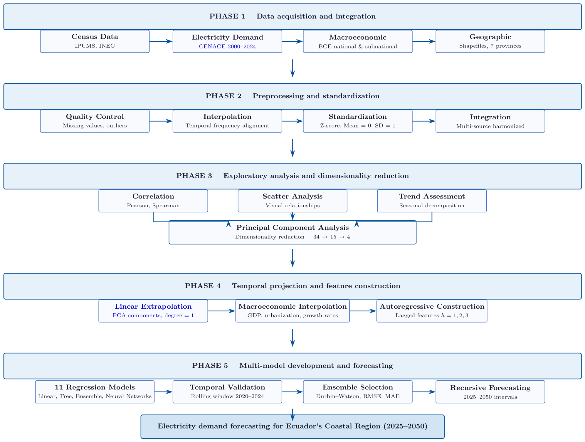
Before describing the Ecuadorian implementation, it is useful to present the methodological pipeline at a general level, so that its logic can be evaluated independently from the specific case study. The framework is designed for territorial contexts in which three information layers are typically available: (i) periodic population and housing census microdata, which provide rich but temporally sparse socioeconomic information; (ii) an official annual electricity demand series at the regional or national level; and (iii) macroeconomic aggregates (for example GDP or sectoral value added) published at annual frequency. The pipeline is organized in five sequential stages, summarized in Figure 1 and detailed in Figure 2.
In the first stage, census microdata from different rounds are harmonized into a common set of territorial indicators covering demographic structure, household composition, housing quality, access to basic services and educational attainment. In the second stage, Principal Component Analysis is applied to this harmonized matrix to obtain a small number of orthogonal components that summarize the main axes of territorial heterogeneity, reducing multicollinearity and allowing a compact representation of development patterns. In the third stage, each retained component (or each selected indicator) is projected to the demand horizon by means of a univariate linear function of calendar year (degree one) to avoid spurious curvature given the limited number of census observations. In the fourth stage, the projected territorial drivers are combined with macroeconomic variables and fitted to a log-transformed demand variable through a set of competing regression specifications, which differ in their functional form and in the subset of predictors. In the fifth stage, model selection and validation rely on rolling-origin backtesting, complemented by a final holdout window, so that predictive performance is evaluated under conditions that approximate real planning use.
The five-stage structure is deliberately simple and transparent, which is a design choice rather than a limitation. In data-scarce environments, more complex models tend to overfit and lose interpretability, whereas the present pipeline produces components and coefficients —namely, loadings and axes of variation— that can be inspected and discussed with domain experts as qualitative directions of territorial change rather than as point forecasts of individual indicators. In methodological terms comparable to Sheng et al., who also relied on PCA-based socioeconomic components [35], and to Boukarta et al., who combined PCA with regression in an urban context [36], the framework emphasizes reproducibility and the ability to be re-estimated whenever new census rounds or updated macroeconomic series become available.

2.2.2. Study Design and Methodological Workflow

Building on the general pipeline introduced above, this subsection describes the specific operational workflow adopted for Ecuador’s Costa region. The study adopted a descriptive-correlational quantitative approach to examine the relationships between territorial development patterns and electricity demand in the region. The methodological strategy was structured as a five-phase analytical pipeline integrating dimensionality reduction, temporal projection, and supervised regression techniques. Figure 2 summarizes the detailed methodological workflow adopted in the study, which comprises: (i) data acquisition and integration, (ii) preprocessing and standardization, (iii) exploratory analysis and dimensionality reduction, (iv) temporal projection and feature construction, and (v) multi-model development and forecasting.

2.2.3. Data Preprocessing and Standardization

Given the heterogeneity of sources and their irregular periodicity, preprocessing was carried out sequentially in four stages. First, records were cleaned through the identification and removal of outliers and incomplete observations. Second, temporal interpolation was applied to transform the discontinuous census observations into continuous annual series. Third, the selected sociodemographic variables were standardized using Z-score transformation, with zero mean and unit variance. Finally, all sources were integrated into a single analytical dataset with temporal coverage spanning 2000–2050.

2.2.4. Exploratory Analysis and Dimensionality Reduction

The analysis was aimed at identifying distribution and interrelation patterns among the explanatory variables. To this end, the Pearson correlation matrix was computed for the 34 original census variables in order to detect collinearity patterns and guide subsequent predictor selection. In addition, scatter plots were constructed for six pairs of territorial indicators selected for their theoretical relevance to electricity demand, incorporating the corresponding correlation coefficient and an ordinary least-squares trend line. This analysis was complemented by time-evolution plots of demographic and basic service coverage indicators, with the aim of characterizing the socioeconomic transformations underlying electricity consumption patterns.
Two assumptions of different nature underlie the framework and should be kept distinct. The PCA stage assumes only that the fifteen standardized census variables lie approximately on a lower-dimensional linear subspace, so that four orthogonal components reproduce the dominant axes of territorial heterogeneity; it makes no assumption about how the scores evolve in time. Four principal components were retained based on cumulative explained variance and the inflection point of the scree plot. The factor loadings and biplot of the first two components were then examined to interpret the latent structure of the data and verify that the census observations are well separated in the reduced space. The subsequent extrapolation of each PC score on the calendar year (used only to feed the comparator models; see Section 2.2.7) is implemented as a univariate linear regression. A quadratic specification was tested during model development but produced divergent end-of-horizon behaviour, which is why we restricted the projection to degree one.

2.2.5. Temporal Projection and Feature Construction

Since the principal component scores were available only at five census points, each retained component was projected to the 2000–2050 horizon using univariate linear regression on the calendar year. A quadratic specification was tested at the development stage but absorbed idiosyncratic noise of the 2010 round and produced divergent end-of-horizon behaviour, so the projection was restricted to degree one. The projected components were subsequently combined with independently interpolated macroeconomic indicators and three lagged variables of the target variable, corresponding to demand at t 1 , t 2 , and t 3 .

2.2.6. Multi-Model Development, Validation, and Forecasting

Eleven regression algorithms grouped into different model families were evaluated. All specifications were estimated on electricity demand transformed using the natural logarithm, in order to stabilize series variance, ensure positive predictions upon back-transformation, and facilitate interpretation of results in terms of relative growth.
Model performance was evaluated using rolling-origin backtesting and a holdout validation period corresponding to 2020–2024. The selection procedure was hierarchical: (i) a plausibility filter discarded any model whose 2025–2050 trajectory implied a non-positive compound annual growth rate; (ii) among the remaining candidates, models with a positive coefficient of determination on the 2020–2024 holdout window were preferred; and (iii) within that subset, the model with the lowest holdout RMSE was selected. The Durbin–Watson statistic on the backtest residuals is reported as a diagnostic complement but was not used as a primary selection criterion. The recommended model was then refitted on the full 2000–2024 demand series and projected recursively through 2050.

2.2.7. Formal Specification of the Pipeline

For reproducibility and to facilitate re-estimation of the framework in other emerging economies, the main operational steps are summarized in compact notation. Let y t denote the annual regional electricity demand (MW) in year t, and let t 0 be the first year of the historical sample.
After standardization of the 15 retained socioeconomic variables, Principal Component Analysis was applied to the pooled census matrix, yielding four components PC i ( c ) scored at each round c { 1974 , 1982 , 1990 , 2001 , 2010 } . Because only five observations are available per component and the forecast horizon extends four decades beyond the last census, each score was extrapolated to 2000–2050 by a
univariate linear regression on the calendar year,
PC ^ i ( t ) = α i , 0 + α i , 1 t , i = 1 , , 4 .
A linear trajectory was preferred over higher-degree polynomials because, with only five census points, quadratic extrapolation produces divergent behavior at long horizons.
The forecasting models operate on the log-transformed demand series t = log ( y t ) . The general specification of the pipeline combines a linear trend on the calendar year, the four projected components, and a vector of macroeconomic indicators m t = ( GDP t , IND t , PopGr t ) (per capita GDP, industrial index, and annual population growth rate),
t = β 0 + β τ ( t t 0 ) + i = 1 4 β i PC ^ i ( t ) + γ m t + ε t ,
with ε t a zero-mean error term. The eleven estimators evaluated share this predictor structure and differ only in their estimation rule: unpenalized least squares, ridge, lasso, ElasticNet, Huber, linear-kernel SVR, polynomial-ridge (degree 2 on the same inputs), spline-ridge (cubic B-spline transformation), and two tree-based nonparametric regressors (random forest and gradient boosting). The autoregressive variant, ARX-ridge, extends Equation (2) with three lags of log-demand,
t = β 0 + β τ ( t t 0 ) + i = 1 4 β i PC ^ i ( t ) + γ m t + k = 1 3 ϕ k t k + ε t ,
and is the only specification that incorporates past demand explicitly.
The role of the projected principal components in the framework is therefore confined to the comparator models defined by Equations (2) and (3). The recommended specification, in contrast, depends only on the calendar year and on the annual electricity demand series; its long-horizon projection does not require any extrapolation of the census-derived components beyond 2010.
The recommended model, Trend OLS log, corresponds instead to the parsimonious restriction of Equation (2) in which only the trend term is retained,
t = β 0 + β τ ( t t 0 ) + ε t ,
fitted by ordinary least squares on the 2000–2019 training window and projected recursively to 2050.
Temporal generalization was assessed through rolling-origin backtesting. For each origin t * within the historical window, the model was re-estimated using the expanding sample { ( x s , s ) : s t * } and used to predict t * + 1 , so that every test point remained strictly out of sample. The 2020–2024 window was reserved entirely as an independent holdout and did not enter any training or hyperparameter-tuning stage.
Predictive accuracy was summarized on the MW scale after back-transforming the predictions as y ^ t = exp ( ^ t ) , using the root mean squared error, the mean absolute percentage error, and the coefficient of determination,
RMSE = 1 n t = 1 n y t y ^ t 2 , MAPE = 100 n t = 1 n y t y ^ t y t , R 2 = 1 t = 1 n y t y ^ t 2 t = 1 n y t y ¯ 2 .
A positive R 2 on the holdout window therefore indicates that the model outperforms the sample-mean predictor over 2020–2024. The Durbin–Watson statistic was additionally reported as a residual diagnostic in the results that follow.

3. Results

3.1. Exploratory Analysis, Dimensionality Reduction, and Socioeconomic Projections

The historical electricity demand series for Ecuador’s Costa region (2000–2024) shows a sustained, nearly monotonic growth trajectory. Demand increased from 1076.1 MW in 2000 to 2914.1 MW in 2024, with an average of 1914.3 MW. Overall, this behavior represents a compound annual growth rate (CAGR) of 4.24% and a cumulative increase of 170.8%, associated with economic expansion, rising consumption, and advances in urbanization and industrialization. The only year-on-year contractions were observed between 2016 and 2017, in line with the macroeconomic adjustment recorded in that period. Also notable is the acceleration during the holdout validation window (2020–2024), whose CAGR reached 7.70% above the historical average and consistent with a stronger post-pandemic recovery.
The census database used to construct structural predictors encompasses 34 socioeconomic variables observed at five census points between 1974 and 2010. These variables were grouped into four thematic domains: (i) household structure and demographics, (ii) access to basic services and infrastructure, (iii) education, employment, and gender composition, and (iv) connectivity and telecommunications. From these 34 raw indicators, 15 variables were retained for the PCA on the basis of a four-step protocol: (i) exclusion of non-predictor fields, namely the calendar-year index and the demand target itself; (ii) substitution of raw counts by their corresponding normalized rates, whenever both were available, to prevent the analysis from loading on indicators mechanically correlated with population size; (iii) removal of the complementary half of binary splits (for example, the female population share as the complement of the male share) to avoid perfect linear dependence in the correlation matrix; and (iv) reduction in the four educational-attainment categories to a single rate, the share of tertiary-educated population, the most discriminating dimension for residential and commercial demand modelling [13,14,35]. The resulting selection (Table 1) is exhaustive: any variable not listed in Table 1 falls under one of the four exclusion rules above. Table A1 in Appendix A reports the rule applied to each of the 34 raw indicators. The temporal evolution of these variables across the five censuses is presented in Table 1.
The temporal evolution of the selected variables indicates substantial transformations during the 1974–2010 period. In Domain I, the mean number of persons per household decreased by 34.5% (from 7.30 to 4.78), while population density increased by 51.6% (from 54.00 to 81.88 inhab/km2), evidencing a sustained process of household nucleation and urban expansion. In Domain II, basic service coverage indicators show the most pronounced changes: electricity access nearly doubled ( + 104.3 % , from 47.0% to 96.0%) and access to drinking water tripled ( + 224.2 % , from 18.0% to 58.3%), reflecting the sustained infrastructure investment effort by the Ecuadorian state. In Domain III, the proportion with university education experienced the largest relative increase from 1.0% to 6.3%, albeit from an extremely low base marking the process of mass expansion of higher education. Domain IV (connectivity) started from zero values in 1974 and 1982, with internet penetration reaching 29.0% in 2010 and mobile telephony 11.6%, exhibiting exponential growth dynamics unmatched in any other domain.
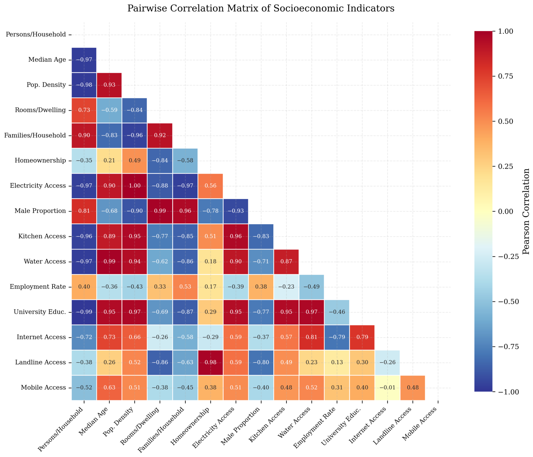
Pearson correlation analysis applied to the 34 original socioeconomic variables revealed strong inter-predictor dependence, particularly among demographic, infrastructure, and socioeconomic activity groups. Examining the subset of 15 selected variables yielded 105 possible bivariate pairs, of which 41 (39.0%) exhibited | r | > 0.80 , 25 (23.8%) exceeded | r | > 0.90 , and 18 (17.1%) reached | r | > 0.95 . Taken together, these results confirm high redundancy among variables and justify the application of PCA as a strategy to reduce multicollinearity and synthesize system information (Figure 3).
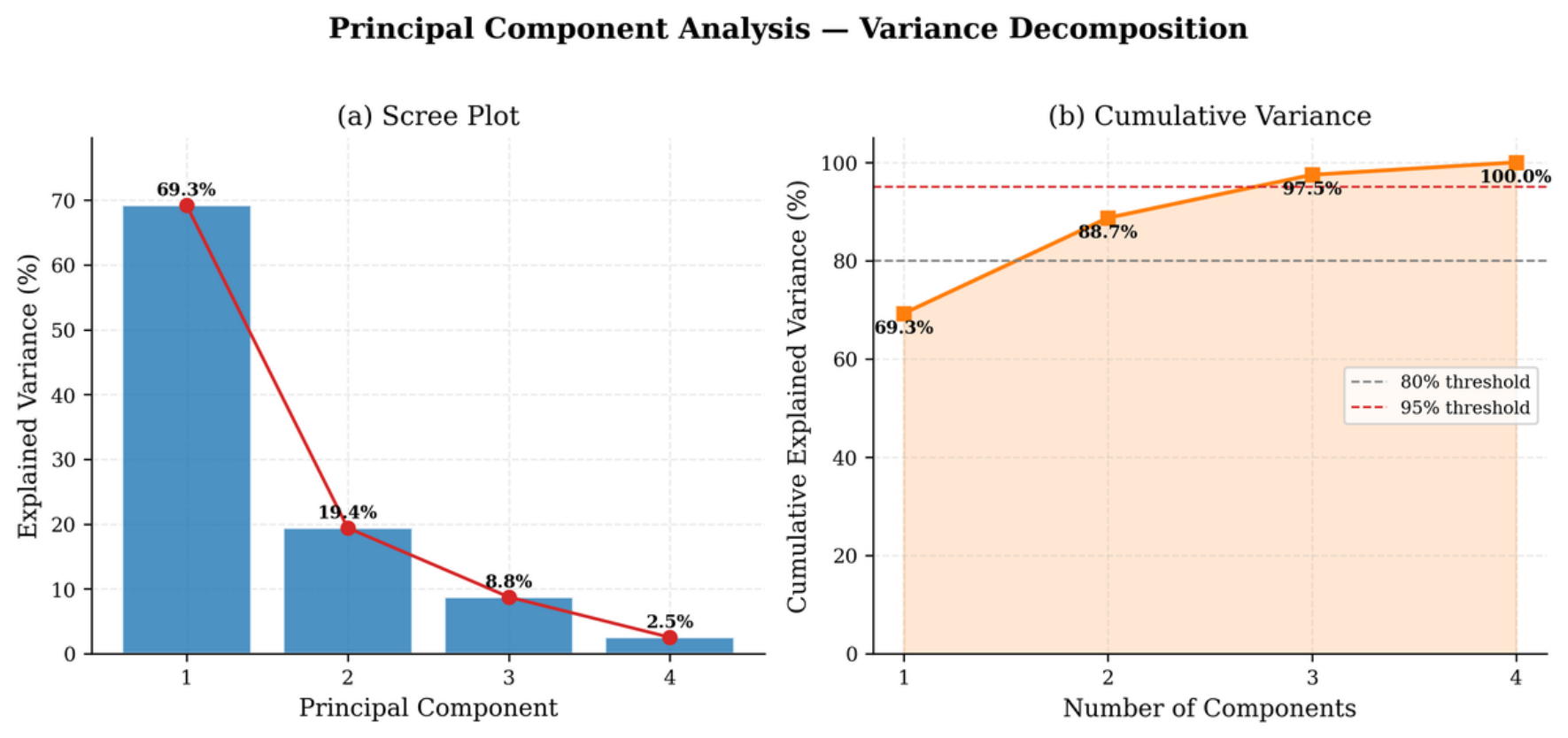
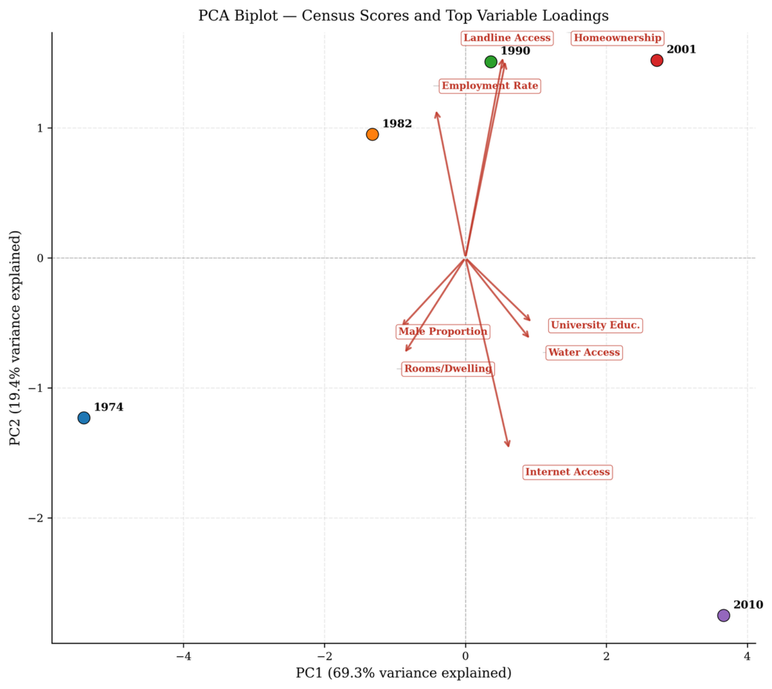
PCA applied to these 15 variables yielded four principal components (PC1–PC4) with eigenvalues above 0.8. PC1 explained 69.26% of total variance, PC2 19.44%, PC3 8.77%, and PC4 2.53%, with the first two components jointly accounting for 88.70% and all four retained components for 100% of the variance (Figure 4). The loading structure indicates that PC1 is primarily defined by variables linked to socioeconomic modernization, access to basic services, and housing conditions, while PC2 represents a secondary dimension of differentiation associated with demographic, employment, and connectivity variables, as illustrated in the biplot (Figure 5).
The temporal projection of component scores through 2050 was performed via univariate linear regression of each component against the census year. PC1 showed a high fit ( R 2 = 0.929 ; slope = 0.241 score/year), indicating a consistent temporal trend that supports its extrapolation under a stability criterion. PC2, PC3, and PC4 showed considerably lower fits ( R 2 < 0.06 ); their future trajectories were therefore estimated using a conservative approach with slope restriction, in order to limit speculative divergence arising from long-horizon extrapolation with a limited number of observations. These projected trajectories, combined with independently extrapolated macroeconomic variables (per capita GDP, industrial index, and the annual population growth rate), formed the vector of exogenous predictors used across the full set of forecasting models.

3.2. Model Fit During the Training Period

For electricity demand projection, eleven model specifications were implemented, all estimated on demand transformed using the natural logarithm. Several models achieved high in-sample fit during the training phase, but performance was not uniform under temporal validation. Gradient Boosting achieved a near-perfect training fit ( R 2 1.000 ) but showed a substantial drop in backtesting accuracy, a pattern clearly indicative of overfitting. In contrast, regularized models Ridge, Lasso, ElasticNet, and Huber exhibited more stable behavior and a better balance between in-sample fit and out-of-sample predictive capacity, a result consistent with the constraints imposed by the training sample size.

3.2.1. Model Performance in Temporal Backtesting

Rolling-origin backtesting, based on iterative retraining of each model using information available up to each test point within the historical period, allowed evaluation of temporal generalization capacity under a prospective scheme. As shown in Table 2, Gradient Boosting recorded the lowest backtesting RMSE (93.34 MW), followed by Spline-Ridge (98.41 MW) and ARX-Ridge (109.01 MW). The Durbin–Watson statistic showed heterogeneous residual autocorrelation patterns: Trend OLS ( D W = 0.172 ) and Poly2-Ridge ( D W = 0.027 ) exhibited strong positive autocorrelation, while Gradient Boosting ( D W = 1.981 ), Spline-Ridge ( D W = 1.945 ), and Random Forest ( D W = 1.705 ) showed more temporally independent residuals.

3.2.2. Temporal Holdout Validation (2020–2024)

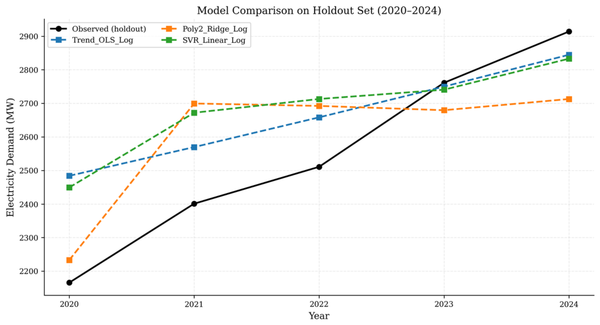
The 2020–2024 period was reserved entirely for holdout evaluation, with no involvement in any training phase or hyperparameter selection. Electricity demand increased from 2165.6 MW in 2020 to 2914.1 MW in 2024 a cumulative increase of 34.6% and a CAGR of 7.70%, clearly above the long-run historical trend (4.24%). This increase, partly attributable to post-pandemic economic reactivation and the expansion of rural electrification, constituted a relevant challenge for models calibrated exclusively on pre-2020 information (Figure 6).
Under this scenario, only three models achieved a positive coefficient of determination in the holdout set (the minimum condition to outperform the naive reference predictor): Trend OLS log ( R 2 = 0.551 , RMSE = 176.9 MW, MAPE = 6.08 % ), Poly2-Ridge log ( R 2 = 0.502 , RMSE = 186.4 MW, MAPE = 6.53 % ), and SVR Linear log ( R 2 = 0.422 , RMSE = 200.8 MW, MAPE = 7.19 % ). The remaining eight models exhibited negative R 2 , with RMSE ranging from 364.9 MW to 823.7 MW, reflecting the inability of highly penalized models to adapt to the structural acceleration of post-2020 demand from macroeconomic predictors projected in advance.
Annual analysis of the recommended model (Table 3) shows systematic overestimation in 2020–2022, with errors between + 5.9 % and + 14.7 % , attributable to the transient demand decline during the pandemic not anticipated by the macroeconomic predictors. From 2023 onward, the error decreases markedly, reaching 0.4 % in 2023 and 2.4 % in 2024. This behavior indicates that Trend OLS log consistently reproduces the long-run structural trajectory, although with lower sensitivity to short-term shocks.

3.2.3. Selection Criteria and Recommended Model

The selection of the long-horizon projection model followed the three-stage hierarchical procedure introduced in Section 2.2.7. First, models whose projected 2025–2050 trajectories implied a non-positive CAGR were discarded, as this behavior is inconsistent with the expected population growth and electrification expansion in Ecuador: Spline-Ridge (CAGR = 0.17 % ), Random Forest ( 0.36 % ), and Gradient Boosting ( 0.02 % ) were eliminated by this filter. Second, among the remaining candidates, models with a positive coefficient of determination on the 2020–2024 holdout window were prioritized, since this criterion best reflects predictive capacity in the most recent period. Third, within that subset, the model with the lowest holdout RMSE was selected.
Under this procedure, Trend OLS log was identified as the most appropriate specification. It combined a coherent prospective trajectory, a positive holdout R 2 (0.551), and the lowest RMSE in the evaluated set (MAPE = 6.08 % ). Although its log-linear structure is less flexible than other specifications, it provides a stable and monotonic trajectory that reduces the risk of erratic behavior during extrapolation. A methodological limitation should be explicitly acknowledged: the Durbin–Watson statistic from backtesting ( D W = 0.172 ) indicates positive first-order residual autocorrelation which, while it does not invalidate the central projection, suggests interpreting the results with appropriate caution. Poly2-Ridge log ranked as the second most consistent alternative ( R 2 = 0.502 ), albeit with a more expansive projection toward 2050.

3.2.4. Long-Horizon Electricity Demand Forecast (2025–2050)

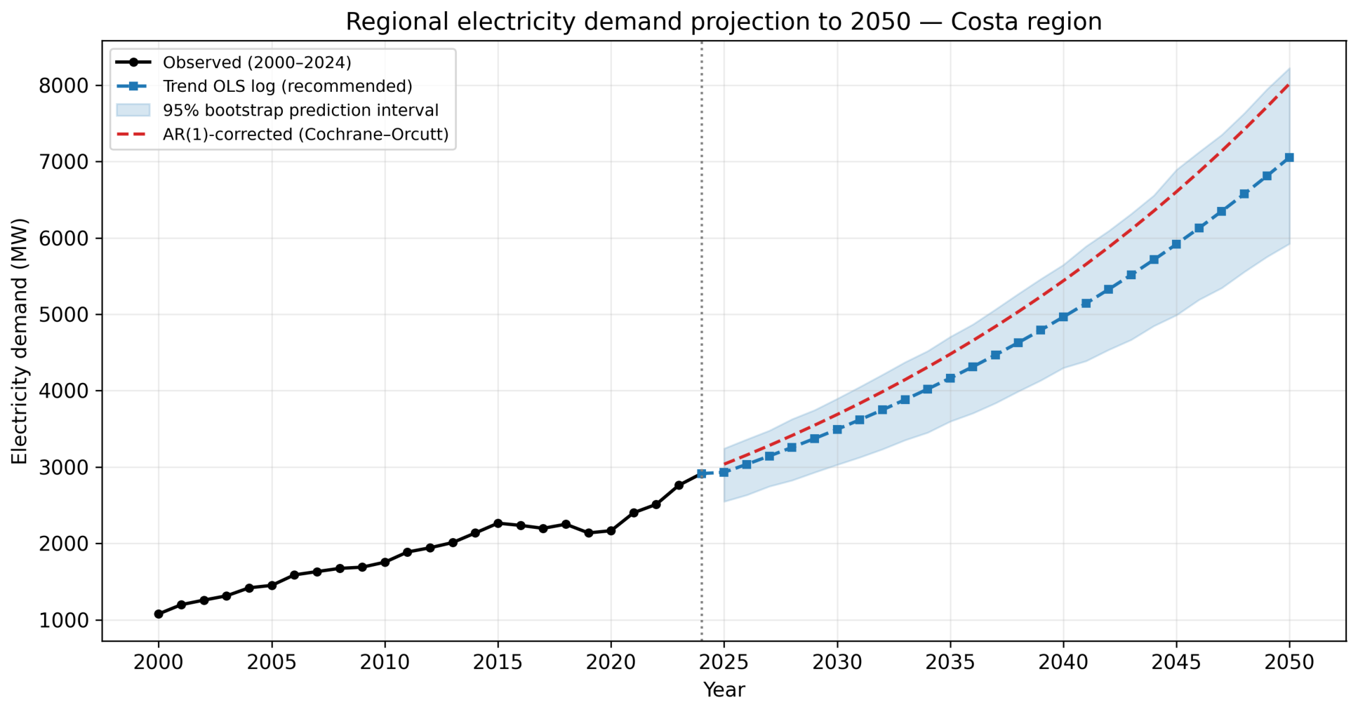
The selected model projects regional electricity demand for Ecuador’s Costa region at 2930.5 MW for 2025, equivalent to a 0.56% increase over the value observed in 2024 (2914.1 MW)—a continuous transition between the historical series and the projected trajectory, with no abrupt breaks at the start of the forecast horizon. The projection maintains a path of moderate growth, reaching 3493.4 MW in 2030, 4964.3 MW in 2040, and 7054.6 MW in 2050, corresponding to a CAGR of 3.46% for 2024–2050. This pace is lower than that observed in 2020–2024 (7.70%) and slightly below the long-run historical trend (4.24%), suggesting a gradual deceleration toward a more stable growth trajectory (Figure 7).
The two uncertainty bands reported in Figure 7 and Table 4 answer different questions. The 95% bootstrap prediction interval of the recommended model captures parameter and innovation uncertainty under the assumption that the structural conditions of 2000–2024 continue; its half-width grows from ± 11.8 % in 2025 to ± 16.3 % in 2050. The inter-model envelope, in turn, quantifies the additional dispersion attributable to model-class choice; its width at 2050 (from 4714 to 9453 MW) reflects the fact that long-horizon forecasts in data-scarce settings are sensitive to specification. The bootstrap interval should therefore be read as a probabilistic interval conditional on the trend specification, and the inter-model envelope as a scenario range describing the additional uncertainty attributable to the choice of regression family.

3.2.5. Comparative Scenarios Across All Valid Models

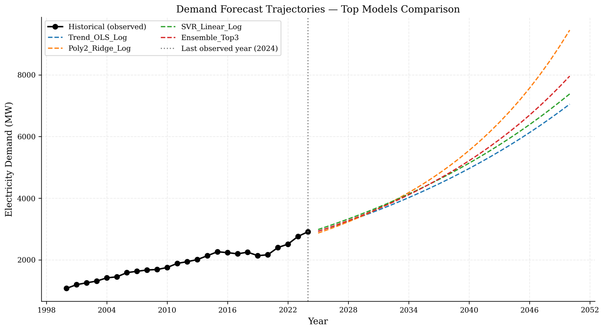
Comparative analysis of the projections generated by all valid models reveals significant divergence across long-horizon scenarios (Table 5). In aggregate, the eight plausible models estimate electricity demand for 2050 ranging from 4713.5 MW to 9453.4 MW, a spread of 4739.9 MW. This dispersion reflects the high uncertainty inherent in long-horizon energy projection exercises, particularly in contexts where historical data availability is limited and the future trajectory depends on structural and macroeconomic variables subject to change. At intermediate horizons, divergence is already significant: for 2040, valid projections range approximately from 3548.0 to 5549.3 MW, a difference of 2001.3 MW (Figure 8).
Within this set, the recommended model Trend OLS log projects 7054.6 MW for 2050 with a CAGR of 3.46%, placing it in an intermediate-to-high position within the range. Its estimate exceeds the more conservative scenarios, such as ARX–Ridge log (4713.5 MW; 1.87%), ElasticNet log (5368.5 MW; 2.38%), and Ridge log (6438.1 MW; 3.10%), but falls below the more expansive trajectories represented by Huber log (7931.2 MW; 3.93%) and, especially, Poly2–Ridge log (9453.4 MW; 4.63%). This intermediate position is substantively relevant, as it represents a projection consistent with a moderate growth scenario that avoids both excessive underestimation and overly aggressive demand expansion.
The three models generating decreasing scenarios (Random Forest, Gradient Boosting, and Spline-Ridge) were excluded from the final selection. Their projections for 2050 (2654–2898 MW) fall below the value observed in 2024, a result inconsistent with projected population growth, the progressive expansion of electricity coverage, and the electrification dynamics anticipated for Ecuador over the analysis horizon.

3.2.6. Residual Diagnostics

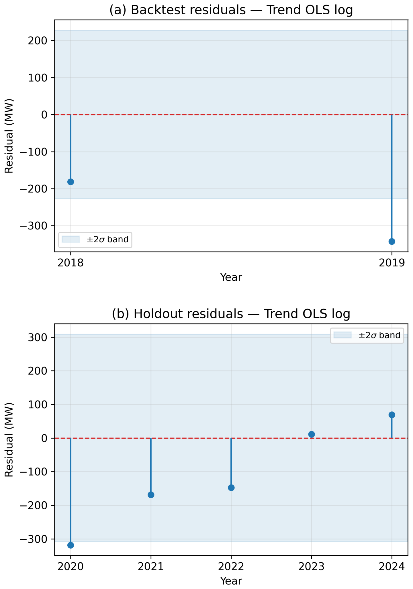
The residual diagnostics of the recommended model (Trend OLS log) show systematic overestimation during the backtesting period, with a residual mean of 261.8 MW and a standard deviation of 113.6 MW. This indicates that the model tended to project values above those observed, behavior consistent with its trend-based nature in the face of a series that still exhibits cyclical variations not captured by the log-linear specification. In the holdout period (2020–2024), this pattern changes: the initial overestimation decreases gradually until converging toward actual values in 2023, with moderate underestimation appearing in 2024 (Figure 9). Taken together, these patterns suggest that the model did not fully anticipate the post-pandemic demand acceleration, although it did converge toward the observed trajectory in the most recent years.
The Durbin–Watson statistic from backtesting ( D W = 0.172 ) confirms the presence of positive first-order residual autocorrelation, indicating that the log-linear formulation does not capture the full temporal dependence of the series. This limitation increases the uncertainty of bootstrap-estimated intervals, so the 95% CI should be interpreted as a conservative planning band rather than a precise probabilistic bound. Residual diagnostics in the holdout period show no systematic long-run deviation after 2022, consistent with the model’s gradual convergence toward actual values. Two implications follow for the long-horizon results. First, under positively autocorrelated errors the ordinary least squares estimator remains unbiased and consistent but ceases to be efficient in the Gauss–Markov sense, and its conventional variance estimator is biased downward; the resulting standard errors and confidence intervals are therefore optimistic, and the 2050 figure should be read as a conditional-mean trajectory rather than a precise point estimate. Second, because the h-step-ahead forecast-error variance of a trend specification with first-order autoregressive disturbances grows with the horizon, the discrepancy between nominal and empirical interval coverage widens toward 2050, which is why the long-horizon estimates are bounded by the inter-model envelope rather than reported in isolation. The generalized least squares re-estimation reported below, which restores efficiency by modeling the autoregressive error structure explicitly, confirms that the central trajectory is robust, so the projections are presented as planning references rather than strict probabilistic bounds.
To assess whether the residual autocorrelation flagged by the Durbin–Watson statistic distorts the long-run signal, the Trend OLS log specification was re-estimated by iterative Cochrane–Orcutt generalized least squares. The procedure recovers a first-order autoregressive coefficient ρ ^ = 0.814 and raises the full-sample Durbin–Watson statistic from 0.43 to 1.61 on the transformed residuals (the value of 0.172 reported in Table 2 is the rolling-origin backtesting statistic, computed on a different validation scheme), indicating that the linear trend captures the conditional mean once the autoregressive error structure is accommodated. The corrected coefficient implies an annual growth rate of 3.96% (95% confidence interval [3.23%, 4.70%]) and a 2050 projection of 8020 MW, slightly above the central 7054.6 MW obtained from the trend model without the autocorrelation adjustment but well within the inter-model envelope of Figure 8. Following Politis and White [37], the prediction intervals reported in Table 4 are additionally recomputed with a circular block bootstrap, yielding an autocorrelation-aware 95% interval of [6369; 10,149] MW at 2050. The projection without the autocorrelation adjustment is retained as the central reference for comparability with the comparator models, while the autoregressive-corrected trajectory is presented as a plausible and equally defensible alternative.

4. Discussion

The performance of the recommended model (MAPE = 6.08 % in the validation period) should be interpreted in light of data availability. This error level falls within a range comparable to that reported by Mado et al. [38], Vargas-Forero et al. [39], and Hamsa et al. [40] for ARIMA models in contexts with short series. More complex approaches tend to outperform simple specifications when longer series and richer predictor datasets are available [39,40,41,42,43], yet this pattern changes when the sample is small. Makris et al. [44] show that, in data-scarce scenarios, simpler models can match or even outperform more complex alternatives. This reading aligns with the warning issued by Hippert and Taylor [45] regarding the risk of overfitting and model selection instability in short series. In this context, the fact that a log-linear specification exhibited the most stable behavior in this study should not be interpreted as a methodological limitation, but rather as a coherent response to a problem in which the main constraint is not algorithmic capacity but sample size. In methodological terms comparable to Sheng et al., who also relied on PCA-based socioeconomic components [35], the use of only five census observations as the support for structural predictors limited out-of-sample generalization capacity, even for the most flexible methods. This result is also consistent with the findings of Rúales and Jaramillo et al. [46], who obtained low errors with parsimonious models in Ecuadorian applications.
A second relevant finding is the incorporation of territorial and socioeconomic factors through PCA, in combination with macroeconomic variables and demand lags. Unlike approaches based solely on aggregate indicators, this strategy made it possible to condense a dense and highly interrelated structure linked to income, urbanization, infrastructure access, household size, and connectivity into a small number of components, dimensions widely recognized as determinants of electricity demand [39]. In this regard, the results are consistent with those reported by Sheng et al. [35] and Boukarta et al. [36], who also used PCA to synthesize relevant socioeconomic variables in demand studies. In this study, PC1 and PC2 concentrated the bulk of the variance and provided a consistent reading of the structural modernization process of the Costa region. This finding reinforces the idea that demand expansion depends not only on aggregate macroeconomic changes, but also on long-run territorial and social transformations. In this sense, the results converge with prior work emphasizing the relevance of population density and socioeconomic development in explaining subnational energy consumption [46,47]. Moreover, the internal heterogeneity of the Costa region suggests differentiated trajectories across provinces: while territories such as Guayas, with greater urbanization and industrialization, will likely continue to concentrate a significant share of aggregate demand, other provinces with relatively lower coverage could exhibit faster growth rates as electrification advances [47].
The 2020–2024 validation period also introduced a particularly relevant element: a recent demand acceleration that no model fully captured. The CAGR of 7.70% well above the historical trend suggests an inflection point associated with post-pandemic reactivation, advances in electrification, and the effects of the recent energy crisis [48,49]. This behavior contrasts with simple trend projections that assume continuity in historical patterns, and confirms as already cautioned by Ruales and Jaramillo [46] that atypical events can substantially alter demand dynamics and exceed the explanatory capacity of traditional models. From a planning perspective, this finding reinforces the need to interpret long-horizon projections as plausible trajectories rather than immutable point estimates. Under this logic, the breadth of the projected range for 2050 does not constitute a weakness of the analysis, but a valuable input for designing robust decisions in generation, transmission, and distribution [50,51].
Nevertheless, the results must be interpreted with caution. The structural basis of the model rests on only five census observations, excludes the 2022 census due to comparability issues, works with aggregated regional demand, and does not incorporate climatic variables, despite their relevance in tropical systems [52]. Added to this is the positive residual autocorrelation of the recommended model ( D W = 0.172 ), indicating that part of the temporal dependence was not fully absorbed by the specification. This finding is consistent with Serrano et al. [53] and Aditya et al. [54], who show that an unresolved residual structure can widen projection intervals and compromise their coverage; the iterative Cochrane–Orcutt correction reported in Section 3 (yielding ρ ^ = 0.814 and a transformed D W = 1.61 ) addresses precisely this concern, and the AR(1)-aware block-bootstrap interval of Table 4 reflects the resulting widening. For this reason, the projections and their intervals should be treated primarily as a reference for strategic planning, rather than as strict probabilistic bounds. Along these lines, future studies should incorporate climatic variables, deepen the sectoral and territorial disaggregation of demand, and update the structural base with new comparable data sources.
A direct consequence of the design choice described in Section 2.2.7 is that the long-horizon projection of the recommended model is robust to the temporal sparsity of the censuses, but it inherits the standard limitation of any trend specification: it assumes that the conditions that sustained 3–4% annual growth in 2000–2024 (steady electrification, population growth, residual industrial expansion) will continue to operate. The principal components PC1–PC4 should therefore be read as inertia-driven summaries of slow-moving territorial change rather than as forward-looking forecasts of individual indicators. Variables that follow saturating dynamics (such as electricity access, already close to its natural ceiling at the 2010 census) or non-linear adoption curves (such as internet and mobile telephony, whose 2010 levels still mark inflection points rather than steady states) cannot be expected to evolve linearly beyond the last census round, so the linear extrapolation is treated as a working approximation rather than as a calibrated projection of each underlying indicator. Crucially, this residual uncertainty is absorbed only by the comparator models reported in Table 2 (which the holdout filter discards) and not by the recommended specification, which depends solely on the annual demand series and on the calendar year.
The empirical results for the Costa region should be read jointly with the methodological design presented in Section 2.2.1. The selected Trend OLS log specification, with R 2 = 0.551 and MAPE = 6.08 % , is not presented as the best possible model in absolute terms, but as the most defensible specification given the available information. In contexts with richer predictor sets and longer high-frequency series, more sophisticated approaches, such as state-space models or machine-learning regressors, tend to outperform simple log-linear specifications [44,45]. Yet, when the sample is small and the territorial signal comes from widely spaced censuses, parsimonious models with a limited number of interpretable coefficients are often preferable, because they reduce the risk of overfitting and remain auditable by planning authorities.
A second element that deserves attention is the sensitivity of long-term projections to the linear extrapolation of territorial drivers. Restricting the projection of each component score to a univariate linear trend (degree one), as described in Section 2.2.5, is a conservative choice that prevents implausible curvature at the end of the horizon. Even so, the projected demand of approximately 7054.6 MW by 2050 and the implied CAGR of 3.46% should be interpreted as a central trajectory conditional on the continuation of historical development patterns, rather than as a point forecast. This is consistent with the way similar PCA-based exercises have framed their results in other developing contexts [35,36], and with the cautionary notes raised by Arnob and Wang for countries with limited data [20,22].
Finally, the framework contributes to the Ecuadorian planning literature by complementing studies that have focused on reliability, generation mix or scenario-based energy modeling [5,23,46]. Rather than replacing those approaches, the proposed pipeline provides a territorial front-end that can feed any of them, by translating slow-moving census information into synthetic indicators that are comparable across rounds and projectable over time.

4.1. Comparison with Official Instruments and Recent Energy-Planning Studies in Ecuador

The official planning instrument for Ecuador’s electricity sector is the Electricity Master Plan, which defines national guidelines for electricity demand, generation, and system expansion [33]. Since this instrument and recent national studies operate at the country level, whereas the present study focuses specifically on Ecuador’s Coastal Region, the comparison is framed as an external plausibility check rather than as a direct validation in absolute MW values.
The recommended projection for the Coastal Region shows a compound annual growth rate of 3.46% over the 2024–2050 period. This trajectory is consistent with the general direction of recent national studies, which emphasize the need for capacity expansion, diversification of the electricity mix, and strengthened system resilience. In this regard, Naranjo-Silva et al. [23], using a national LEAP-based model, project minimum installed capacity requirements between 22,990 MW and 27,095 MW by 2050, depending on the scenario considered. Although these values refer to the national system and not to regional demand, they confirm a structural trend of growth and expansion in Ecuador’s electricity sector.
Similarly, Cevallos and Urquizo [47] develop a spatially enabled national multi-period model for Ecuador’s electricity system over the 2020–2035 horizon. Their study uses LEAP to assess demand and generation scenarios, incorporating assumptions from the Electricity Master Plan, singular loads, industrial projects, electric transport, and new generation projects. In their results, the authors use a demand growth rate close to 5.44% between 2020 and 2035 and estimate national electricity demand of up to 89,380 GWh in 2035 under the highest-expansion scenario.
In this context, the regional growth rate estimated in the present study is more moderate than the medium-term national trajectories, which is reasonable given the differences in scale, time horizon, and modeling assumptions. Therefore, the comparison with official instruments and recent studies supports the general plausibility of the projected trajectory for the Coastal Region, but it should not be interpreted as a direct comparison in MW. An absolute validation would require officially disaggregated regional projections or an explicit methodology for allocating national demand across territories.

4.2. Transferability to Other Emerging Economies

The pipeline described in Section 2.2.1 is intentionally agnostic about the country of application, and its core ingredients are available in many emerging economies. The transferability of the framework, however, is not automatic and depends on several conditions that should be checked on a case-by-case basis. First, at least a few census rounds with comparable variables must be available, so that harmonization and PCA can produce stable components; when only one or two rounds are available, the territorial signal tends to be too weak to support regression-based projection. Second, the demand series should be sufficiently long and free from major structural breaks unrelated to territorial development, such as large tariff reforms or prolonged rationing episodes, which would otherwise dominate the fit. Third, macroeconomic aggregates should be available at annual frequency and at a level of disaggregation that is consistent with the spatial scope of the analysis.
When these conditions are met, the pipeline can be re-estimated with local data without modifying its structure. Countries in the Andean region, Central America and parts of Southeast Asia share with Ecuador a combination of rapid urbanization, structural transformation and limited high-frequency statistics [20,26], which makes the framework potentially useful for their medium- and long-term planning. Where these conditions are only partially met, the same pipeline can still be used as a diagnostic tool, by highlighting which territorial drivers carry most of the explanatory weight and which would require additional data collection before being used for projection.

5. Conclusions

This article proposed and applied a reproducible exploratory framework to analyze the interactions between territorial development patterns and electricity demand in contexts where high-frequency socioeconomic information is scarce. At a general level, the framework combines census harmonization, PCA-based synthesis of territorial indicators, linear projection of drivers, multi-model log-linear regression and rolling-origin validation into a single, auditable pipeline. At an applied level, it was instantiated on Ecuador’s Costa region using five non-uniform census rounds (1974, 1982, 1990, 2001, 2010) and the official annual demand series.
Among the eleven specifications compared, the Trend OLS log model emerged as the most defensible compromise between fit and parsimony, with R 2 = 0.551 and MAPE = 6.08 % on the holdout window. Under the assumption that historical development trajectories continue, the model projects a regional demand of approximately 7054.6 MW by 2050, equivalent to a compound annual growth rate of 3.46%. This result implies an increase of 142.1% relative to 2024 and confirms the need for sustained expansion of generation, transmission, and distribution infrastructure. These figures should be read as a central planning signal rather than as a deterministic forecast, and the breadth of the scenario range toward 2050 reinforces that planning should rely on a range of plausible trajectories rather than on a single point estimate.
The main contribution of the work is methodological. By making each stage of the pipeline explicit and testable, the framework offers planners and researchers in other emerging economies a transparent template that can be re-estimated whenever new census rounds or updated macroeconomic aggregates become available. Future work will focus on extending the framework to other Ecuadorian regions, on incorporating climatic variables where reliable series exist, on deepening the analysis at the provincial scale, on integrating the 2022 census once its comparability inconsistencies have been resolved, and on comparing the present specification with state-space and machine-learning alternatives once longer high-frequency records are released.


Author Contributions

Conceptualization, D.P.; methodology, D.P.; software, D.P.; validation, D.P., J.M. and F.O.; formal analysis, D.P.; investigation, D.P.; resources, D.P.; data curation, D.P.; writing original draft preparation, D.P. and Y.O.; writing review and editing, D.P., Y.O., C.L.-A. and F.J.; visualization, D.P.; supervision, F.J.; project administration, D.P.; funding acquisition, J.M. All authors have read and agreed to the published version of the manuscript.

Funding

This research received no external funding. The article processing charge (APC) was waived by the publisher.

Institutional Review Board Statement

Not applicable.

Informed Consent Statement

Not applicable.

Data Availability Statement

Data supporting the reported results are available upon reasonable request to the corresponding author. Census microdata were obtained from IPUMS International (https://international.ipums.org, accessed on 8 April 2026) and INEC (https://www.ecuadorencifras.gob.ec, accessed on 8 April 2026). Electricity demand data are available in CENACE annual reports (https://www.cenace.gob.ec, accessed on 8 April 2026).

Acknowledgments

The authors would like to thank IPUMS International, INEC, CENACE, and the Central Bank of Ecuador for providing the data used in this study.

Conflicts of Interest

The authors declare no conflicts of interest.

Abbreviations

The following abbreviations are used in this manuscript:
PCAPrincipal Component Analysis
BCECentral Bank of Ecuador
CAGRCompound Annual Growth Rate
DWDurbin–Watson statistic
GDPGross Domestic Product
PopGrAnnual population growth rate
HDIHuman Development Index
HOHoldout
LEAPLong-range Energy Alternatives Planning
LSTMLong Short-Term Memory
MAPEMean Absolute Percentage Error
RMSERoot Mean Square Error
SNINational Interconnected System
SVRSupport Vector Regression

Appendix A. Variable Selection Protocol

Table A1 documents, indicator by indicator, the application of the four-step selection protocol described in Section 3 to the 34 raw census indicators. The rules are: R1, exclusion of non-predictor fields; R2, substitution of a raw count by its corresponding normalized rate when both are available; R3, removal of the complementary half of a binary split; and R4, reduction in the educational-attainment categories to the single most discriminating rate. Nineteen indicators are excluded (two by R1, thirteen by R2, one by R3 and three by R4) and fifteen are retained, exactly those listed in Table 1.
Table A1. Variable-by-variable application of the 34-to-15 selection protocol; “Rule” is the exclusion criterion, retained indicators enter the PCA.
#IndicatorDecisionRuleReason
1Calendar year (time index)DropR1Not a socioeconomic indicator; used as the time coordinate.
2Households owning their dwelling (count)DropR2Superseded by the homeownership rate.
3Households not owning their dwelling (count)DropR2Superseded by the homeownership rate.
4Persons per householdRetainDirect indicator of household nucleation.
5Median age of populationRetainDirect indicator of demographic structure.
6Population density (inhab./km2)RetainDirect indicator of territorial density.
7Households with electricity (count)DropR2Superseded by the electricity-access rate.
8Households without electricity (count)DropR2Superseded by the electricity-access rate.
9Male population (count)DropR2Superseded by the male-proportion rate.
10Female population (count)DropR2Superseded by the male-proportion rate.
11Rooms per dwellingRetainDirect indicator of housing quality.
12Households without a kitchen (count)DropR2Superseded by the kitchen-access rate.
13Households with a kitchen (count)DropR2Superseded by the kitchen-access rate.
14Households with drinking water (count)DropR2Superseded by the drinking-water-access rate.
15Households without drinking water (count)DropR2Superseded by the drinking-water-access rate.
16Families per householdRetainDirect indicator of household composition.
17Employed population (count)DropR2Superseded by the employment rate.
18Unemployed population (count)DropR2Superseded by the employment rate.
19Population with less than primary education (count)DropR4Lower-level educational share collinear with its complement.
20Population with primary education (count)DropR4Lower-level educational share collinear with its complement.
21Population with secondary education (count)DropR4Lower-level educational share collinear with its complement.
22Population with tertiary education (count)DropR2Superseded by the tertiary-education rate.
23Electricity demand (target variable)DropR1Regression target, not a predictor.
24Internet access (rate)RetainDirect indicator of connectivity.
25Landline telephone access (rate)RetainDirect indicator of telecommunications.
26Mobile telephone access (rate)RetainDirect indicator of mobile telecommunications.
27Homeownership (rate)RetainReplaces the owner/non-owner counts (R2).
28Electricity access (rate)RetainReplaces the electrified/non-electrified counts (R2).
29Male proportion (rate)RetainReplaces the male/female counts (R2).
30Female proportion (rate)DropR3Exact complement of the male proportion.
31Kitchen access (rate)RetainReplaces the kitchen presence/absence counts (R2).
32Drinking-water access (rate)RetainReplaces the water presence/absence counts (R2).
33Employment (rate)RetainReplaces the employed/unemployed counts (R2).
34Tertiary-education share (rate)RetainMost discriminating educational level (R4).

References

  1. Peplinski, M.; Dilkina, B.; Chen, M.; Silva, S.J.; Ban-Weiss, G.A.; Sanders, K.T. A Machine Learning Framework to Estimate Residential Electricity Demand Based on Smart Meter Electricity, Climate, Building Characteristics, and Socioeconomic Datasets. Appl. Energy 2024, 357, 122413. [Google Scholar] [CrossRef] [Scilit]
  2. Tang, W.; Wang, H.; Lee, X.-L.; Yang, H.-T. Machine Learning Approach to Uncovering Residential Energy Consumption Patterns Based on Socioeconomic and Smart Meter Data. Energy 2022, 240, 122500. [Google Scholar] [CrossRef] [Scilit]
  3. Carrillo, C.D.B.; Pilatuña, P.W.P.; Chicaiza, Q.C.I. Forecasting Energy Consumption in the Chimborazo Province, Ecuador, Using Random Forest and XGBoost Algorithms. In Proceedings of the 2023 1st International Conference on Advanced Engineering and Technologies (ICONNIC), Kediri, Indonesia, 13–14 October 2023; pp. 66–72. [Google Scholar] [CrossRef] [Scilit]
  4. Parra-Jácome, R.M.; Yánez-Jácome, G.B.; Pinto-Arteaga, G.R.; Rea-Toapanta, A.R. Consumos Heterogéneos de Energía en las Tipologías de Hogares del Sector Residencial del Ecuador. FIGEMPA Investig. Desarro. 2024, 17, 102–111. [Google Scholar] [CrossRef] [Scilit]
  5. Peña, D.; Téllez, A.A.; Jurado, F. Reliability Assessment of Ecuador’s Power System: Metrics, Vulnerabilities, and Strategic Perspectives. Energies 2025, 18, 3059. [Google Scholar] [CrossRef] [Scilit]
  6. Cheng, L.; Zang, H.; Xu, Y.; Wei, Z.; Sun, G. Probabilistic Residential Load Forecasting Based on Micrometeorological Data and Customer Consumption Pattern. IEEE Trans. Power Syst. 2021, 36, 3762–3775. [Google Scholar] [CrossRef] [Scilit]
  7. Clements, A.E.; Hurn, A.S.; Li, Z. Forecasting Day-Ahead Electricity Load Using a Multiple Equation Time Series Approach. Eur. J. Oper. Res. 2016, 251, 522–530. [Google Scholar] [CrossRef] [Scilit]
  8. Rawal, K.; Ahmad, A. Feature Selection for Electrical Demand Forecasting and Analysis of Pearson Coefficient. In Proceedings of the 2021 IEEE 4th International Electrical and Energy Conference (CIEEC), Wuhan, China, 28–30 May 2021; pp. 1–6. [Google Scholar] [CrossRef] [Scilit]
  9. Chen, P.-C.; Kezunovic, M. Load Consumption Prediction Utilizing Historical Weather Data and Climate Change Projections. In Proceedings of the 2017 19th International Conference on Intelligent System Application to Power Systems (ISAP), San Antonio, TX, USA, 17–20 September 2017; pp. 1–6. [Google Scholar] [CrossRef] [Scilit]
  10. Jawad, M.; Nadeem, M.S.A.; Shim, S.-O.; Khan, I.R.; Shaheen, A.; Habib, N.; Hussain, L.; Aziz, W. Machine Learning Based Cost Effective Electricity Load Forecasting Model Using Correlated Meteorological Parameters. IEEE Access 2020, 8, 146847–146864. [Google Scholar] [CrossRef] [Scilit]
  11. Salas-Monteros, J.M.; Maldonado-Navarro, J.L.; Llerena-Poveda, V.d.C.; Alban-Navarro, S.F. Evolución del Consumo y Generación de Energía Eléctrica en Ecuador: Análisis del Balance Energético y Diversificación de la Matriz Energética (2021–2024). Rev. Investig. Talent. 2025, 12, 1–16. [Google Scholar] [CrossRef] [Scilit]
  12. Chicaiza-Yugcha, O.F.; Martínez-Guaman, C.J.; Orozco-Manobanda, I.A.; Arellano-Castro, Á.D. Previsión del Consumo Eléctrico en el Cantón Salcedo Mediante Técnicas de Aprendizaje Automático. Rev. Odigos 2024, 5, 9–24. [Google Scholar] [CrossRef] [Scilit]
  13. Sun, H.; Han, B. Regional Power Grid Load-Forecast Considering Socio-Economic Factors. In Proceedings of the 2023 2nd International Conference on Advanced Electronics, Electrical and Green Energy (AEEGE), Singapore, 26–28 May 2023; pp. 70–74. [Google Scholar]
  14. Karuparthi, Y.; Shoaib, S.H.; Kommareddi, H.C.; Jothi, J.A.A. Predicting Energy Demand with Interpretable Machine Learning Models. In Proceedings of the 2024 International Conference on Artificial Intelligence, Metaverse and Cybersecurity (ICAMAC), Dubai, United Arab Emirates, 25–26 October 2024; pp. 1–6. [Google Scholar]
  15. Jasiński, T. A New Approach to Modeling Cycles with Summer and Winter Demand Peaks as Input Variables for Deep Neural Networks. Renew. Sustain. Energy Rev. 2022, 159, 112217. [Google Scholar] [CrossRef] [Scilit]
  16. Shiwakoti, R.K.; Charoenlarpnopparut, C.; Chapagain, K. A Deep Learning Approach for Short-Term Electricity Demand Forecasting: Analysis of Thailand Data. Appl. Sci. 2024, 14, 3971. [Google Scholar] [CrossRef] [Scilit]
  17. Yajure-Ramírez, C.A. Pronóstico de Consumo de Energía Eléctrica Residencial de Corto Plazo Utilizando Algoritmos de Aprendizaje Automático y Profundo. Rev. Investig. Sist. Informát. 2022, 15, 23909. [Google Scholar] [CrossRef] [Scilit]
  18. Abiodun, A.A.; Tosho, A.; Kamil, S.K. Prediction Model for Electricity Energy Consumption and Pricing Using XGBoost with L1 Regularization. Kasu J. Comput. Sci. 2024, 1, 640–652. [Google Scholar] [CrossRef] [Scilit]
  19. Safari, A.; Kharrati, H.; Rahimi, A. VoltaVistaMan: Energy Dynamics Intelligent Predictive Analysis. In Proceedings of the 2024 IEEE International Conference on Prognostics and Health Management (ICPHM), Spokane, WA, USA, 17–19 June 2024; pp. 316–322. [Google Scholar] [CrossRef] [Scilit]
  20. Arnob, S.S.; Arefin, A.I.M.S.; Saber, A.Y.; Mamun, K.A. Energy Demand Forecasting and Optimizing Electric Systems for Developing Countries. IEEE Access 2023, 11, 39751–39775. [Google Scholar] [CrossRef] [Scilit]
  21. Hassan, H.; Xiaoying, W.; Sampene, A.K.; Xu, L. The Socio-Economic and Technological Dimensions of Energy Transition. Energy Strategy Rev. 2025, 62, 101895. [Google Scholar] [CrossRef] [Scilit]
  22. Wang, B.; Fu, Q.; Lu, Y.; Liu, K. Limited Data Availability in Building Energy Consumption Prediction. Information 2025, 16, 575. [Google Scholar] [CrossRef] [Scilit]
  23. Naranjo-Silva, S.; Punina-Guerrero, D.J.; Jacome-Dominguez, E.A.; Escobar-Segovia, K.; Laverde-Albarracín, C. Energy Planning Under Climate Pressure in Ecuador: Insights from the 2023–2024 Crisis Using LEAP Modeling. Sustainability 2026, 18, 2112. [Google Scholar] [CrossRef] [Scilit]
  24. Moya, D.; Copara, D.; Borja, A.; Pérez, C.; Kaparaju, P.; Pérez-Navarro, Á.; Giarola, S.; Hawkes, A. Geospatial and Temporal Estimation of Climatic, End-Use Demands, and Socioeconomic Drivers of Energy Consumption in the Residential Sector in Ecuador. Energy Convers. Manag. 2022, 261, 115629. [Google Scholar] [CrossRef] [Scilit]
  25. Araujo-Vizuete, G.; Robalino-López, A.; Mena-Nieto, Á. Looking beyond Subsidies: Understanding the Complexity of Household Energy Consumption Dynamics of Ecuador’s Main Cities. Cities 2025, 163, 106008. [Google Scholar] [CrossRef] [Scilit]
  26. Icaza-Alvarez, D.; Jurado, F.; Tostado-Véliz, M. Smart Energy Planning for the Decarbonization of Latin America and the Caribbean in 2050. Energy Rep. 2024, 11, 6160–6185. [Google Scholar] [CrossRef] [Scilit]
  27. Bhattacharyya, S.C.; Timilsina, G.R. A Review of Energy System Models. Int. J. Energy Sect. Manag. 2010, 4, 494–518. [Google Scholar] [CrossRef] [Scilit]
  28. Suganthi, L.; Samuel, A.A. Energy Models for Demand Forecasting—A Review. Renew. Sustain. Energy Rev. 2012, 16, 1223–1240. [Google Scholar] [CrossRef] [Scilit]
  29. Hyndman, R.J.; Athanasopoulos, G. Forecasting: Principles and Practice, 3rd ed.; OTexts: Melbourne, Australia, 2021. [Google Scholar]
  30. Debnath, K.B.; Mourshed, M. Forecasting Methods in Energy Planning Models. Renew. Sustain. Energy Rev. 2018, 88, 297–325. [Google Scholar] [CrossRef] [Scilit]
  31. IPUMS International. Citation of IPUMS International. Available online: https://international.ipums.org/international/citation.shtml (accessed on 8 April 2026).
  32. Instituto Nacional de Estadística y Censos. Resultados del Censo Nacional de Población; INEC: Quito, Ecuador, 2022; pp. 1–62. [Google Scholar]
  33. Medina, J. Operador Nacional de Electricidad—CENACE; CENACE: Quito, Ecuador, 2024; pp. 1–220. [Google Scholar]
  34. Mundial, B. PIB per Cápita (UMN Actual). Available online: https://datos.bancomundial.org/indicador/NY.GDP.PCAP.CN (accessed on 8 April 2026).
  35. Sheng, Y.; Liu, J.; Wei, D.; Song, X. Heterogeneous Study of Multiple Disturbance Factors Outside Residential Electricity Consumption: A Case Study of Beijing. Sustainability 2021, 13, 3335. [Google Scholar] [CrossRef] [Scilit]
  36. Boukarta, S.; Berezowska-Azzag, E. Assessing Households’ Gas and Electricity Consumption: A Case Study of Djelfa, Algeria. Quaest. Geogr. 2018, 37, 111–129. [Google Scholar] [CrossRef] [Scilit]
  37. Politis, D.N.; White, H. Automatic Block-Length Selection for the Dependent Bootstrap. Econom. Rev. 2004, 23, 53–70. [Google Scholar] [CrossRef] [Scilit]
  38. Mado, I.; Rajagukguk, A.; Triwiyatno, A.; Fadllullah, A. Short-Term Electricity Load Forecasting Model Based DSARIMA. Int. J. Electr. Energy Power Syst. Eng. 2022, 5, 6–11. [Google Scholar] [CrossRef] [Scilit]
  39. Vargas-Forero, V.M.; Manotas-Duque, D.F.; Trujillo, L. Comparative Study of Forecasting Methods to Predict the Energy Demand for the Market of Colombia. Int. J. Energy Econ. Policy 2024, 15, 65–76. [Google Scholar] [CrossRef] [Scilit]
  40. Hamsa, H.; Asem, A.; El-Bakry, H. Advanced Time Series Forecasting Models for Electricity Demand Prediction: A Comparative Study. Fusion Pract. Appl. 2024, 15, 19–31. [Google Scholar] [CrossRef] [Scilit]
  41. Ko, D.; Yoon, Y.; Kim, J.; Choi, H. Effective Electricity Demand Prediction via Deep Learning. IEIE Trans. Smart Process. Comput. 2021, 10, 483–489. [Google Scholar] [CrossRef] [Scilit]
  42. Saha, E.; Saha, R.; Mridha, K. Short-Term Electricity Consumption Forecasting: Time-Series Approaches. In Proceedings of the 2022 10th International Conference on Reliability, Infocom Technologies and Optimization (ICRITO), Noida, India, 13–14 October 2022; pp. 1–5. [Google Scholar] [CrossRef] [Scilit]
  43. Mardotillah, N.A.; Hasanah, R.N.; Wijono. DE-Optimized Hybrid ARIMA-LSTM for Long Term Electricity Load Forecasting. J. Electr. Electron. Commun. Control Inform. Syst. 2025, 19, 39–45. [Google Scholar] [CrossRef] [Scilit]
  44. Makris, I.; Moschos, N.; Radoglou-Grammatikis, P.; Andriopoulos, N.; Tzanis, N.; Malamaki, K.-N.; Fotopoulou, M.; Kaousias, K.; Tompros, G.L.; Sarigiannidis, P. Exploring Load Forecasting: Bridging Statistical Methods to Deep Learning Techniques. In Proceedings of the 2024 20th International Conference on Distributed Computing in Smart Systems (DCOSS-IoT), Abu Dhabi, United Arab Emirates, 29 April–1 May 2024; pp. 491–496. [Google Scholar]
  45. Hippert, H.S.; Taylor, J.W. An Evaluation of Bayesian Techniques for Controlling Model Complexity and Selecting Inputs in a Neural Network for Short-Term Load Forecasting. Neural Netw. 2010, 23, 386–395. [Google Scholar] [CrossRef] [Scilit] [PubMed]
  46. Ruales, J.; Jaramillo, M. Medium-Term Electric Network Planning Using SARIMA: EERSA Case Study—Ecuador. In Proceedings of the 2024 11th International Conference on Power and Energy Systems Engineering (CPESE), Nara City, Japan, 6–8 September 2024; pp. 27–32. [Google Scholar] [CrossRef] [Scilit]
  47. Cevallos, B.; Urquizo, J. Spatial National Multi-Period Long-Term Energy and Carbon Planning Scenarios in Ecuador’s Electric System. J. Environ. Manag. 2024, 370, 122010. [Google Scholar] [CrossRef] [Scilit] [PubMed]
  48. Abdurohman, M.; Putrada, A.G. Forecasting Model for Lighting Electricity Load with a Limited Dataset Using XGBoost. Kinetik Game Technol. Inf. Syst. Comput. Netw. Comput. Electron. Control 2023, 8, 571–580. [Google Scholar] [CrossRef] [Scilit]
  49. Galván, A.; Haas, J.; Moreno-Leiva, S.; Osorio-Aravena, J.C.; Nowak, W.; Palma-Benke, R.; Breyer, C. Exporting Sunshine: Planning South America’s Electricity Transition with Green Hydrogen. Appl. Energy 2022, 325, 119569. [Google Scholar] [CrossRef] [Scilit]
  50. Rodriguez, A.M.B.; Trotter, I.M. Climate Change Scenarios for Paraguayan Power Demand 2017–2050. Clim. Change 2019, 156, 425–445. [Google Scholar] [CrossRef] [Scilit]
  51. Fields, N.; Collier, W.; Kiley, F.; Caulker, D.; Blyth, W.; Howells, M.; Brown, E. Long-Term Forecasting: A MAED Application for Sierra Leone’s Electricity Demand (2023–2050). Energies 2024, 17, 2878. [Google Scholar] [CrossRef] [Scilit]
  52. Trotter, I.M.; Bolkesjø, T.F.; Féres, J.G.; Hollanda, L. Climate Change and Electricity Demand in Brazil: A Stochastic Approach. Energy 2016, 102, 596–604. [Google Scholar] [CrossRef] [Scilit]
  53. Serrano, A.L.M.; Rodrigues, G.A.P.; Martins, P.H.S.; Saiki, G.M.; Filho, G.P.R.; Gonçalves, V.P.; Albuquerque, R.O. Statistical Comparison of Time Series Models for Forecasting Brazilian Monthly Energy Demand. Appl. Sci. 2024, 14, 5846. [Google Scholar] [CrossRef] [Scilit]
  54. Thangjam, A.; Jaipuria, S.; Dadabada, P.K. Model Selection for Long-Term Load Forecasting under Uncertainty. J. Model. Manag. 2024, 19, 2227–2247. [Google Scholar] [CrossRef] [Scilit]
Figure 1. Conceptual five-stage methodological pipeline; its operational instantiation is shown in Figure 2.
Electricity 07 00079 g001
Figure 2. Operational five-phase workflow instantiating the framework of Figure 1 for Ecuador’s Costa region: data integration, preprocessing, dimensionality reduction, feature construction, and demand forecasting.
Electricity 07 00079 g002
Figure 3. Pearson correlation heatmap for the 15 selected socioeconomic variables.
Electricity 07 00079 g003
Figure 4. Principal Component Analysis variance decomposition: (a) scree plot of the explained variance per component, with bar annotations in %; (b) cumulative explained variance with 80% and 95% reference thresholds. The four retained components account for 100% of the variance and are used as inputs for the comparator models.
Electricity 07 00079 g004
Figure 5. PCA biplot (PC1–PC2) of variables and historical censuses.
Electricity 07 00079 g005
Figure 6. Observed demand and holdout predictions (2020–2024) for the three models with positive R 2 .
Electricity 07 00079 g006
Figure 7. Regional demand projection 2025–2050: recommended Trend OLS log central path, 95% bootstrap interval, and AR(1)-corrected trajectory, over the 2000–2024 series.
Electricity 07 00079 g007
Figure 8. Comparative demand projections 2025–2050 for eight plausible models.
Electricity 07 00079 g008
Figure 9. Residual diagnostics of the Trend OLS log model for (a) backtesting and (b) holdout. Each blue marker denotes the annual residual (observed minus predicted demand, in MW); the vertical stem links it to the zero-error reference (dashed red line), and the shaded band spans the ± 2 σ range of the residuals.
Electricity 07 00079 g009
Table 1. Evolution of the 15 PCA variables (1974–2010); proportions in %, Δ = total change 1974–2010.
CodeSocioeconomic Variable19741982199020012010 Δ 1974–2010
Domain I—Household structure and demographics ( n = 5 )
Persons/HouseholdPersons per household7.306.165.404.874.78 34.5 %
Median AgeMedian age (years)22.7323.9824.6526.1828.91 + 27.2 %
Population DensityPopulation density (inhab/km2)54.0060.4265.8372.5581.88 + 51.6 %
Rooms/DwellingRooms per dwelling6.866.015.414.884.27 37.8 %
Families/HouseholdFamilies per household2.522.392.222.132.08 17.3 %
Domain II—Access to basic services and infrastructure ( n = 4 )
Electricity AccessElectricity access (%)47.063.275.889.696.0 + 104.3 %
Water AccessAccess to drinking water (%)18.027.537.951.258.3 + 224.2 %
Kitchen AccessKitchen access (%)73.075.277.179.480.7 + 10.6 %
Homeownership RateHomeownership rate (%)63.063.463.864.365.6 + 4.1 %
Domain III—Education, employment, and gender composition ( n = 3 )
University EducationUniversity education (%)1.01.82.94.56.3 + 534.2 %
Employment RateEmployment rate (%)97.096.495.895.093.8 3.3 %
Male ProportionMale proportion (%)53.052.451.850.950.2 5.2 %
Domain IV—Connectivity and telecommunications ( n = 3 )
Internet AccessInternet access (%)0.00.00.02.129.0 +
Landline AccessLandline telephone (%)0.00.20.82.23.6 +
Mobile Phone AccessMobile phone (%)0.00.00.03.811.6 +
Table 2. Performance of the eleven models (training, backtesting, holdout 2020–2024). RMSE in MW, MAPE in %, DW = Durbin–Watson; (†) recommended model.
ModelTrain R 2 BT RMSEBT MAPEBT DWHO R 2 HO RMSEHO MAPEScenario
Trend OLS log †0.912273.8512.040.1720.551176.906.08Moderate
Poly2 + Ridge log0.899174.407.920.0270.502186.406.53High
SVR Linear log0.857118.924.110.8000.422200.857.19High
ARX + Ridge log0.969109.013.740.918−0.909364.8613.79Conservative
ElasticNet log0.954116.014.611.472−1.374406.9415.65Moderate
Ridge log0.966110.274.341.440−2.293479.1918.32Moderate
Lasso log0.980132.144.731.181−8.211801.4930.01Moderate
Huber log0.979119.114.410.735−8.730823.7530.70High
Spline + Ridge log0.99998.414.411.945−1.185390.3610.84Decreasing *
Random Forest0.981117.204.881.705−1.836444.7114.08Decreasing *
Gradient Boosting1.00093.344.251.981−2.202472.6014.54Decreasing *
BT = rolling-origin backtesting on the CENACE annual demand series, with a minimum training window of 15 years (effective test points 2018 and 2019); HO = temporal holdout on the CENACE demand series 2020–2024, independent of any training or hyperparameter-tuning stage. R 2 < 0 indicates that the model does not outperform the naive predictor. * Models with a Decreasing scenario (CAGR < 0 %) were excluded from the final selection.
Table 3. Holdout predictions (2020–2024) versus actual values for the three models with positive holdout R 2 .
YearActual (MW)Trend OLS †Error (%)Poly2-RidgeError (%)SVR LinearError (%)
20202165.62484.0 + 14.7 2232.8 + 3.1 2449.2 + 13.1
20212401.02569.6 + 7.0 2699.5 + 12.4 2672.0 + 11.3
20222510.82658.3 + 5.9 2692.3 + 7.2 2713.0 + 8.0
20232761.32749.9 0.4 2679.5 3.0 2740.7 0.7
20242914.12844.8 2.4 2712.9 6.9 2833.1 2.8
(†) Recommended model. Negative error values indicate underestimation; positive values indicate overestimation. All three models satisfy the holdout- R 2 > 0 criterion (Section 2.2.7).
Table 4. Regional demand projections (MW), Costa region 2025–2050: central Trend OLS log trajectory, 95% bootstrap prediction interval (B = 2000), and eight-model envelope.
YearCentral (MW)Bootstrap PI 95% (MW)Inter-Model Envelope (MW)
2024 (actual)2914.1
20252930.5[2547.6–3242.1][2521.8–3005.3]
20303493.4[3029.7–3893.6][2769.8–3640.7]
20354164.4[3596.7–4704.7][3124.0–4415.4]
20404964.3[4297.9–5647.1][3548.0–5549.3]
20455917.9[4988.5–6891.6][4064.6–7171.8]
20507054.6[5924.2–8223.7][4713.5–9453.4]
The bootstrap prediction interval is built from a residual and parametric bootstrap of the recommended Trend OLS log model fitted on 2000–2024, with an independent innovation draw at each future horizon. The inter-model envelope reports the year-by-year minimum and maximum across the eight plausible specifications.
Table 5. Projected 2050 demand, cumulative growth and CAGR (2024–2050) for the eleven models. Log-scale models are reported as bias-corrected conditional means; growth is computed against the observed 2024 demand (2914.1 MW).
ModelProj. 2025 (MW)Proj. 2050 (MW)Total Growth (%)CAGR (%)Scenario
Trend OLS log †2930.57054.6 + 142.1 3.46Moderate Electricity 07 00079 i001
Poly2 + Ridge log2871.79453.4 + 224.4 4.63High Electricity 07 00079 i001
SVR Linear log2984.77384.2 + 153.4 3.64High Electricity 07 00079 i001
ARX + Ridge log2521.84713.5 + 61.8 1.87Conservative Electricity 07 00079 i001
ElasticNet log2671.65368.5 + 84.2 2.38Moderate Electricity 07 00079 i001
Ridge log2839.26438.1 + 120.9 3.10Moderate Electricity 07 00079 i001
Lasso log2884.26765.3 + 132.2 3.29Moderate Electricity 07 00079 i001
Huber log3005.37931.2 + 172.2 3.93High Electricity 07 00079 i001
Spline + Ridge log3112.92790.5 4.2 0.17 Decreasing ×
Random Forest2614.82654.9 8.9 0.36 Decreasing ×
Gradient Boosting2878.02898.2 0.5 0.02 Decreasing ×
(†) Recommended model. A check mark (Electricity 07 00079 i001) denotes a model retained as a plausible scenario; a cross (×) denotes a model excluded for implying a non-positive CAGR. Scenarios: conservative (<2.0%), moderate ( 2.0 3.5 % ), high ( 3.5 5.0 % ), decreasing (<0%, excluded).
Disclaimer/Publisher’s Note: The statements, opinions and data contained in all publications are solely those of the individual author(s) and contributor(s) and not of MDPI and/or the editor(s). MDPI and/or the editor(s) disclaim responsibility for any injury to people or property resulting from any ideas, methods, instructions or products referred to in the content.