Stochastic Modeling and Forecasting of Electric Vehicle Charging Demand Using Compound Poisson Processes

Abstract

Electric vehicle (EV) charging demand introduces significant variability in power systems, requiring forecasting approaches capable of representing both aggregated consumption trends and stochastic charging behaviors. While machine learning methods often provide strong predictive performance, they generally require large datasets and substantial computational resources. This paper proposes a stochastic framework based on compound Poisson and Cox processes to model EV charging demand using real charging station data collected at one-minute resolution. The proposed methodology jointly models charging-event arrivals, charging duration, and charging power through probabilistic distributions calibrated from historical observations. A compound homogeneous Poisson process (CHPP) and a double stochastic compound Poisson process (Cox process) are investigated and compared for the generation of synthetic EV charging profiles and short-term forecasting applications. The framework is validated using 1863 charging sessions recorded at a workplace charging infrastructure composed of 37 charging terminals. Monte Carlo simulations are performed to generate synthetic daily charging profiles and evaluate the capability of the models to reproduce key operational indicators, including daily energy consumption and peak grid power demand. The CHPP process achieves average forecasting errors up to 0.8% for daily energy and 6.2% for maximum grid power demand. The results show that Poisson-based stochastic models can generate diverse and realistic charging profiles while requiring only limited historical data and having low computational complexity. The proposed approach provides an interpretable and computationally efficient probabilistic framework for EV charging demand forecasting, synthetic profile generation, and power system operational studies. Stochastic compound Poisson processes may therefore constitute a valuable tool to support the ongoing electrification of mobility and the digital transformation of future smart grids and smart cities.

1. Introduction

The rapid deployment of electric vehicles (EVs) is expected to significantly increase the variability and uncertainty in electricity demand in distribution networks. In France, EV penetration is projected to reach 15.6 million vehicles by 2035, corresponding to an annual electricity consumption of approximately 30 TWh [1]. In parallel, future technologies such as Vehicle-to-Grid (V2G) are projected to provide distributed flexibility services to aggregators and power system operators through the bidirectional control of EV charging stations (EVSEs) and vehicles [2,3]. Accurate EV charging demand forecasting is therefore becoming essential for distribution and transmission system operators, as well as building managers, in order to prevent voltage violations [4], optimize energy losses [5], and improve renewable energy hosting capacity [6].

However, EV charging demand remains highly stochastic due to the diversity and unpredictability of user charging behavior [7]. Practical forecasting and simulation tools should therefore rely on probabilistic frameworks capable of representing charging-event arrivals, charging duration, and charging power demand while remaining computationally efficient and easily adaptable to different charging infrastructures. Since EV charging behaviors strongly depend on the building type, geographical location, and charging infrastructure characteristics, interpretable and lightweight modeling approaches are particularly attractive for practical deployment.

Recent advances in EV charging forecasting have increasingly relied on deep learning and probabilistic forecasting frameworks, including transformer architectures, diffusion models, hierarchical probabilistic approaches, Hawkes processes, and hybrid stochastic-learning frameworks [8,9,10,11,12,13]. Nevertheless, the literature on EV charging demand modeling can generally be divided into three main categories: machine learning approaches, statistical characterization methods, and stochastic process models [14,15]. Machine learning approaches, such as Support Vector Machines (SVMs), Random Forest (RF), gradient boosting methods, and artificial neural networks (ANNs), have been widely investigated for EV charging forecasting [16,17]. Among them, recurrent neural network architectures often provide strong predictive performance for temporal charging profiles [14,18]. However, these approaches generally require large training datasets and substantial computational resources, while their parameters are not directly interpretable from a probabilistic or physical perspective. In addition, EV charging infrastructures often exhibit site-specific characteristics, meaning that trained machine learning models are not necessarily transferable across different charging environments.

Probabilistic EV charging modeling approaches can generally be classified into spatiotemporal methods, queuing-based models, and stochastic temporal models [19]. Queuing theory represents charging stations as service systems, with random arrivals and charging durations, and is particularly suitable for congestion analysis and infrastructure-sizing problems [20]. However, these approaches mainly focus on waiting time analysis rather than the stochastic modeling of charging power demand itself. In the present work, it is assumed that sufficient charging infrastructure is available to limit queuing effects, making stochastic temporal approaches more appropriate for modeling charging events and the associated power demand.

Stochastic temporal models typically rely on combinations of probability distributions describing charging arrival times, charging duration, and charging energy or power demand. For example, Weibull and log-normal distributions have been employed to model charging durations and inter-arrival times [21], while mixtures of Beta distributions and Gaussian mixture models (GMMs) have also been proposed for EV charging characterization [22,23,24,25]. Other studies additionally investigated Gaussian kernel density estimation methods for EV charging demand modeling [6,26].

In office buildings, EV charging arrivals can often be considered as sparse or rare events, making Poisson-based stochastic processes particularly relevant for modeling charging occurrences [25,27,28,29]. Unlike conventional statistical distributions being used independently for arrival time, charging duration, or charging energy, compound Poisson processes provide a unified probabilistic framework capable of jointly modeling charging-event occurrence and load characteristics. In particular, the process intensity directly represents the average number of charging events over a given time interval, providing interpretable model parameters with limited computational complexity.

Although Poisson-based models have already been investigated for EV charging applications, existing studies generally focus on arrival processes only and rarely integrate charging duration and charging power simultaneously. Compound double stochastic Poisson processes (Cox processes), where the intensity itself becomes stochastic, offer additional flexibility for representing time-varying charging behaviors [30]. However, their application to EV charging demand modeling remains largely unexplored and has rarely been validated using real charging datasets. To the best of the authors’ knowledge, few studies have investigated compound Cox processes for the joint stochastic modeling of EV charging arrivals, charging duration, and charging power using real-world charging datasets.

A comparative overview of representative EV charging demand modeling approaches is provided in

Table 1. Comparison of EV charging demand modeling approaches in the literature.

Approach	Main Principle	Advantages	Limitations	Data	Prob.	Interp.	Synthetic Profile Generation
LSTM/deep learning	Temporal sequence learning from historical charging data	High predictive accuracy for large datasets	Requires extensive training data and computational resources; limited interpretability	High	Limited	Low	Limited
Gradient boosting/XGBoost	Supervised learning based on engineered features	Good short-term forecasting performance	Feature engineering required; mostly deterministic outputs	Med–High	Limited	Medium	Limited
Gaussian mixture models (GMMs)	Statistical clustering of charging behaviors	Simple probabilistic representation	Limited capability to represent rare or highly variable events	Medium	Yes	High	Moderate
Hawkes processes	Self-exciting stochastic arrival modeling	Captures temporal dependency between events	Higher model complexity and parameter estimation difficulty	Medium	Yes	Medium	Moderate
Bayesian probabilistic models	Probabilistic inference using prior distributions	Explicit uncertainty representation	Computationally intensive; sensitive to prior assumptions	Med–High	Yes	Medium	Moderate
Conventional Poisson processes	Random independent arrival modeling	Simple and computationally efficient	Limited flexibility for highly variable charging behaviors	Low	Yes	High	Moderate
Proposed compound Poisson/Cox framework	Joint stochastic modeling of arrivals, charging duration and charging power	Interpretable probabilistic framework; low computational cost; suitable for sparse datasets	Assumes event independence and unconstrained charging infrastructure	Low–Med	Yes	High	Strong

. Unlike purely deterministic forecasting methods, the proposed framework focuses on the stochastic generation of realistic charging profiles while maintaining low computational complexity and interpretable model parameters.

The main contribution of this paper is to propose and validate a stochastic framework based on compound Poisson and Cox processes for EV charging demand modeling and forecasting. The proposed methodology jointly models charging-event arrivals, charging duration, and charging power using probabilistic distributions calibrated from real charging data collected in a tertiary building. Two stochastic architectures are investigated and compared: a compound homogeneous Poisson process (CHPP) and a compound double stochastic Poisson process (Cox process). The proposed framework is evaluated using operational grid-related indicators, including daily energy consumption and maximum grid power demand, in order to assess its suitability for synthetic profile generation and power system studies.

The case study relies on real charging data recorded between 2019 and early 2020 from 37 EV charging stations located in a tertiary building and used by 169 heterogeneous EVs. The selected period avoids atypical charging behaviors associated with the COVID-19 pandemic and large-scale remote working policies, which could bias the estimation of stationary stochastic processes. The remainder of the paper is organized as follows. Section 2 introduces the considered Poisson process formulations and associated stochastic modeling framework. Section 3 presents the dataset preprocessing and parameter identification methodology. Section 4 compares and validates the proposed CHPP and Cox-based models using Monte Carlo simulations and operational performance indicators, and further discusses the positioning, limitations, and perspectives of the proposed stochastic forecasting framework.

2. Representing Counting Events with Poisson Processes—Some Generalities

2.1. Presentation

Like electric vehicle charging events, a lot of real-life situations require an explanation or prediction of how many events occur in a given fixed period of time. Events can be deterministic when they are cyclic or periodic, but most of the time they are considered as stochastic processes. In probability theory, point processes are used to capture the random features of events in time. Distributions such as the binomial and Poisson distributions are used in various mathematical models associated with point processes that measure discrete events, but they are definitively quite different. The binomial distribution, Binomial(r,p), with the parameter r being the number of experiments performed and p the probability of success, is able to represent a success/failure outcome in an experiment; while the Poisson distribution, Poisson(λ), where parameter $\lambda$ is the average number of points per some unit, will capture the number of events occurring in a fixed interval of time, area, distance, or volume.

Applications of the Poisson distribution can be found in many fields related to counting, like telecommunications, finance and insurance, astronomy, biology, and earthquakes; see [30] for a review.

The Poisson process, with intensity $\lambda$ ($\lambda >0$), is an occurrence-counting process that satisfies the following conditions:

• The number of occurrences in disjoint time intervals are independent.
• The probability of an occurrence in a small time interval is proportional to the length of this interval, the proportionality coefficient being $\lambda$.
• The probability that there is more than one occurrence in a small time interval is negligible.

These last two conditions are referred to as the “rare event” property. In the literature, it is commonly assumed that if, within a given time interval, $\lambda$ satisfies $3<\lambda <18$, then the underlying assumptions hold. This condition can thus be used to guide the selection of the time frame. Considering a counting process $\{{\mathrm{X}}_{\mathrm{t}};t\ge 0\}$ with a discrete variable ${\mathrm{X}}_{\mathrm{t}}$, a Poisson process has the following properties:

• The standard deviation is equal to the mean:

  $$E\left({\mathrm{X}}_{\mathrm{t}}\right)={\sigma }^2\left({\mathrm{X}}_{\mathrm{t}}\right)=\lambda .$$

  (1)
• Additivity property:
  If $X_1,X_2,...,X_n$ are independent and identically distributed random variables following a Poisson distribution with parameters ${\lambda }_1,{\lambda }_2,...,{\lambda }_n$, respectively, then the sum $X_1+X_2+...+X_n$ also follows a Poisson distribution with a parameter equal to the sum of the individual parameters, $\lambda ={\lambda }_1+{\lambda }_2+...+{\lambda }_n$. The reciprocal is not always valid.

  $$({\displaystyle \sum _{i=1}^n}{X}_i)\sim P({\displaystyle \sum _{i=1}^n}{\lambda }_i).$$

  (2)

Different distributions can be extracted from such processes. An interesting distribution that is closely associated with the arrival time of a basic Poisson process is the inter-arrival time. In this specific case, if times between events are independent and the increments are stationary, then the inter-arrival times are distributed according to an exponential distribution, Exponential($\lambda$), following Equation (3):

$$f(u,\lambda )=\lambda e^{-{\lambda }_u}.$$

(3)

If the arrival of events follows a basic Poisson process with rate $\lambda$, the time until k arrivals follows a gamma distribution $\Gamma (k,\lambda )$ according to Equation (4):

$$g(v,k,\lambda )={\displaystyle \frac{\lambda e^{-\lambda v}{\left(\lambda v\right)}^{k-1}}{(k-1)!}}.$$

(4)

The gamma distribution predicts the time until the $k^{th}$ event occurs. The exponential distribution, on the other hand, predicts the waiting time until the ‘first’ event.

Electric vehicle charging events are difficult to forecast due to their intrinsic characteristics. They are, by nature, totally erratic, due to the behavior of users and the fact that the charging power of each session can also vary. Such events can be modeled through deterministic or stochastic intensity approaches. It is interesting to note that Poisson processes do not require an important dataset or a costly learning procedure, and at the same time assume that events are sporadic.

2.2. Deterministic Intensity

2.2.1. Homogeneous Poisson Process

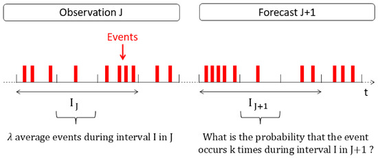
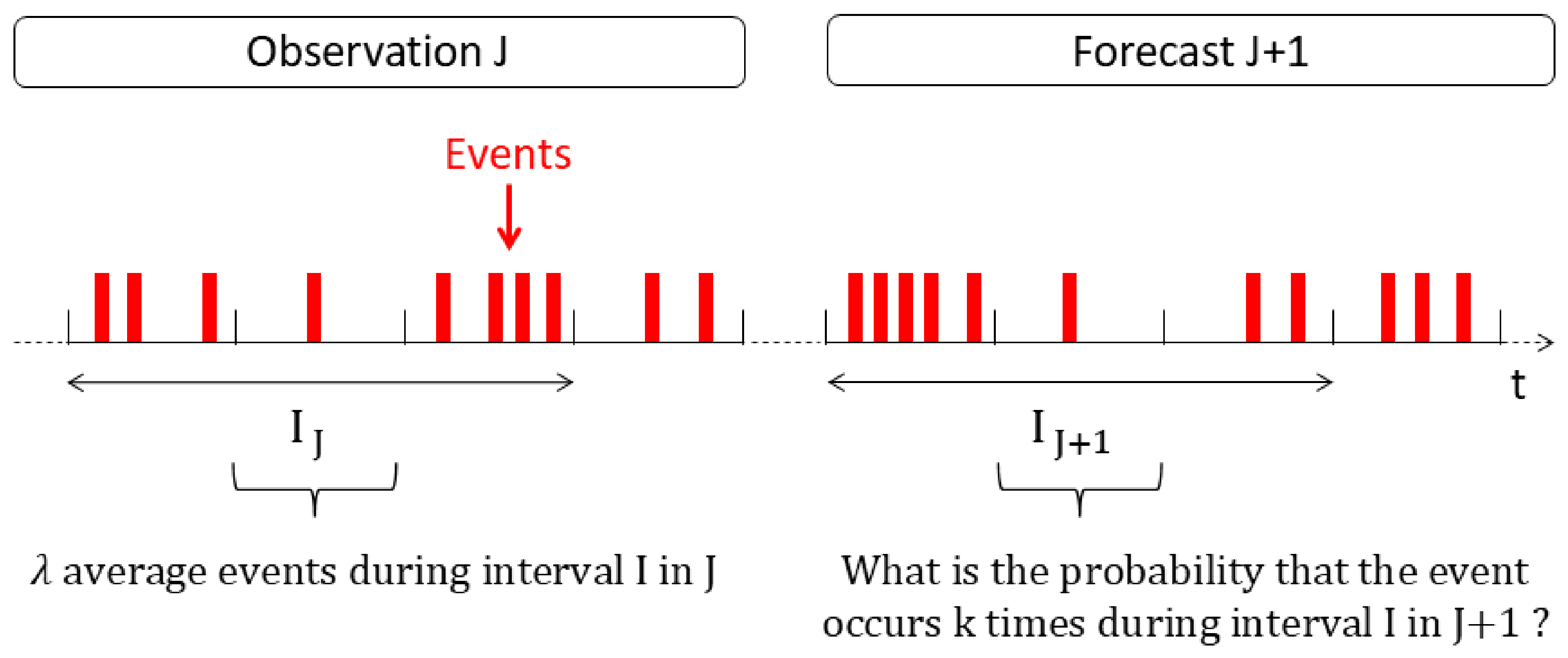
A basic and useful model is the so-called homogeneous Poisson process, in which events occur with a known stationary rate over a bounded period of time, as illustrated in Figure 1.

If a counting process $\{{\mathrm{X}}_{\mathrm{t}};t\ge 0\}$ with a discrete variable ${\mathrm{X}}_{\mathrm{t}}$ has a homogeneous Poisson distribution $P_{X_{\mathrm{t}}}$ with parameter ${\mathrm{X}}_{\mathrm{t}}\ge 0$, then for k = 0, 1, 2, …, the discrete probability density function of ${\mathrm{X}}_{\mathrm{t}}$ is given by Equation (5):

$$\mathbb{P}(X_t=k)={\displaystyle \frac{{\lambda }^k{e}^{-\lambda }}{k!}},\mathrm{with}\lambda =\overline{\lambda }.$$

(5)

As an example, in Figure 1, one could consider that $\lambda$ has an average and stationary value of 8 on interval $I_J$.

2.2.2. Non-Homogeneous Poisson Process

In reality, the occurrences in Figure 1 are not evenly distributed along the time interval $I_J$. So, the intensity can be represented by a deterministic function of time with linear, triangular, polynomial, parabolic, exponential, etc., features. The difference between a homogeneous Poisson process and a non-homogeneous Poisson process lies in the fact that the increments are no longer stationary.

A non-homogeneous Poisson process, on a bounded interval $I_J$, can be described by Equation (6):

$$\mathbb{P}(X_t=k)={\displaystyle \frac{{\lambda }^k{e}^{-\lambda }}{k!}},\mathrm{with}\lambda ={\int }_{I_J}\lambda \left(t\right)dt.$$

(6)

NB: The loss of stationarity also implies that the inter-arrival times are no longer identically distributed according an exponential distribution, Exponential($\lambda$), in Equation (3).

2.3. Stochastic Intensity

In reality, the intensity $\lambda$ itself can be considered as a stochastic variable. Instead of considering a deterministic arrival rate $\lambda$ based on an average value (homogeneous Poisson process) or a function of time (non-homogeneous Poisson process), it is possible to randomize the intensity by using a probability density function.

This specific model is known as a double stochastic Poisson process or Cox process and can be expressed by Equation (7):

$$\mathbb{P}(X_t=k)={\displaystyle \frac{{\lambda }^k{e}^{-\lambda }}{k!}},\mathrm{with}\lambda =h(w,\Lambda ).$$

(7)

The benefit of a random intensity $h(w,\Lambda )$ with a random variable w representing the stochastic intensity and a rate parameter $\Lambda$, lies in the fact that models can take into account additional information, eventually increasing the representativity of the volatility.

2.4. Compound Poisson Process

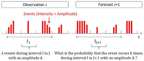
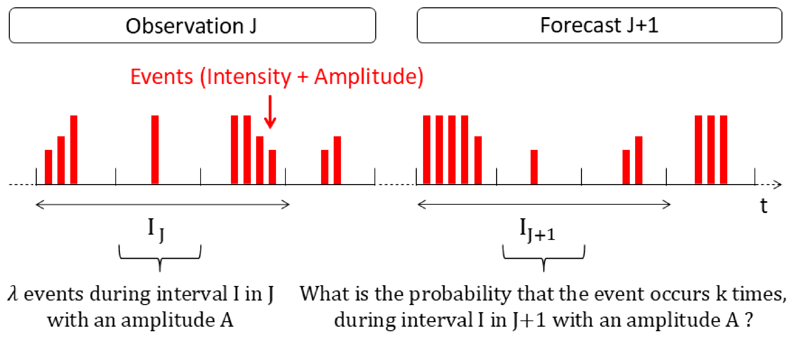
Previous Poisson processes cannot account for two phenomena happening at the same time, as raised in Section 2.1. In a compound Poisson process, Figure 2, each arrival time originally modeled with a counting process $\{{\mathrm{X}}_{\mathrm{t}};t\ge 0\}$, with a discrete variable ${\mathrm{X}}_{\mathrm{t}}$ responding to a Poisson process, comes with an underlying phenomenon $\{{\mathrm{Y}}_{\mathrm{i}};i=1,2,...\}$ corresponding to the amplitude of the event.

The compound Poisson process model considers both the occurrence and the amplitude of events. There are two kinds of representations, one using the cumulative distribution function $C_{df}$ and the other one retrieving the probability density function $P_{df}$ of the amplitude distribution of events $Y_i$ with, respectively, Equation (8) and Equation (9).

• The probability density function $P_{df}$ of $Y_i$ is used to find the probability $P_{X_{\mathrm{t}}}$ that k events occur with an amplitude equal to A:

$$\mathbb{P}(X_t=k,Y=A)={\displaystyle \frac{{\lambda }^k{e}^{-\lambda }}{k!}}{P}_{\mathrm{df}}^{*\left(k\right)}\left(A\right),\mathrm{with}A\ge 0,$$

(8)

• The cumulative distribution function $C_{df}$ of $Y_i$ is used to find the probability $P_{X_{\mathrm{t}}}$ that k events occur with an amplitude equal to or less than A:

$$\mathbb{P}(X_t=k,Y\le A)={\displaystyle \frac{{\lambda }^k{e}^{-\lambda }}{k!}}{C}_{\mathrm{df}}^{*\left(k\right)}\left(A\right),\mathrm{with}A\ge 0.$$

(9)

Many Poisson processes exist and previous classifications are not exhaustive. In any case, Poisson processes could offer a simple way to simulate intermittent loads like electric vehicle charging events, characterizing concomitantly the arrival time and amplitude of events.

3. Modeling EV Charging Events with Poisson Process Structures

3.1. Dataset Description and Preprocessing

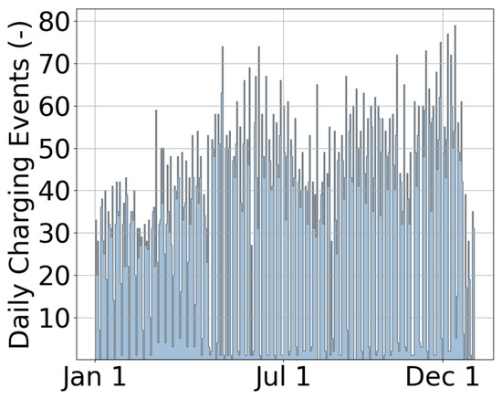
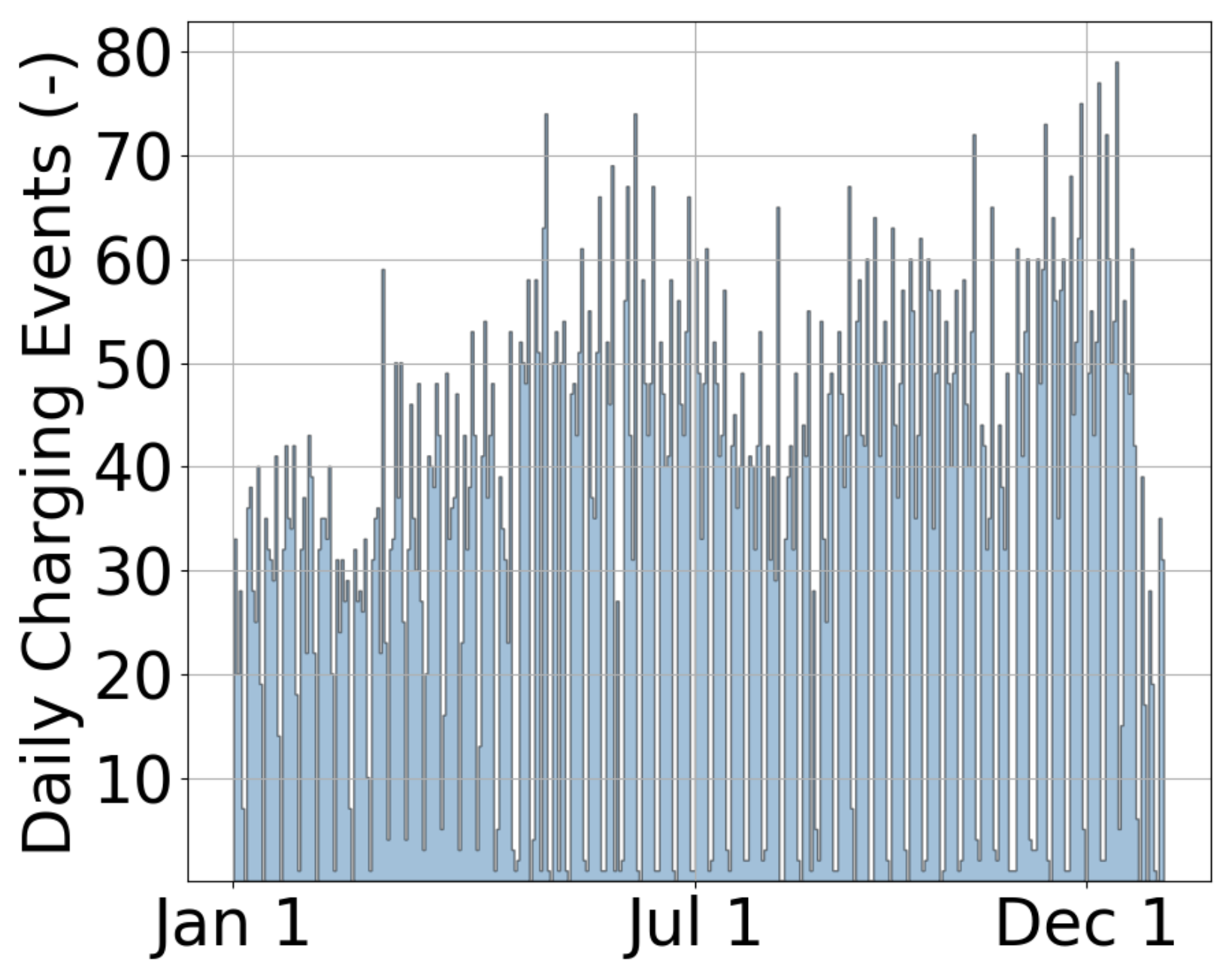
The dataset is available and updated quarterly, on the French Open Data Energy Networks (ODRÉ) platform (https://opendata.reseaux-energies.fr (accessed on 10 october 2019)) that provides stakeholders with data on subjects like “Production”, multi-energy “Consumption”, “Storage”, “Territories and Regions”, “Infrastructures”, “Markets”, and “Meteorology”. The data correspond to all the electric vehicle charging transactions of SAP Labs France employees carried out either at their work place or at home between June 2017 and September 2020. A transaction is the entire operation of charge, from start to stop (from insertion to removal of the badge, button, or cable), including the period of inactivity (when charging is complete but the vehicle is still plugged in). This period was selected in order to avoid atypical charging behaviors associated with the COVID-19 pandemic. The parameter identification in Section 3.2 uses data extracted from the full aforementioned dataset and focuses on the modeling of the starting time, the average power, and the duration of all the charging events in 2019 at the workplace of SAP Lab at Sophia Antipolis. During this year, 11,863 electric vehicle charging events were recorded with a one-minute time step, using thirty-four 22 kW, two 50 kW, and one 150 kW terminals. The resulting daily charging activity during 2019 is illustrated in Figure 3.

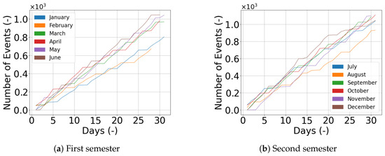
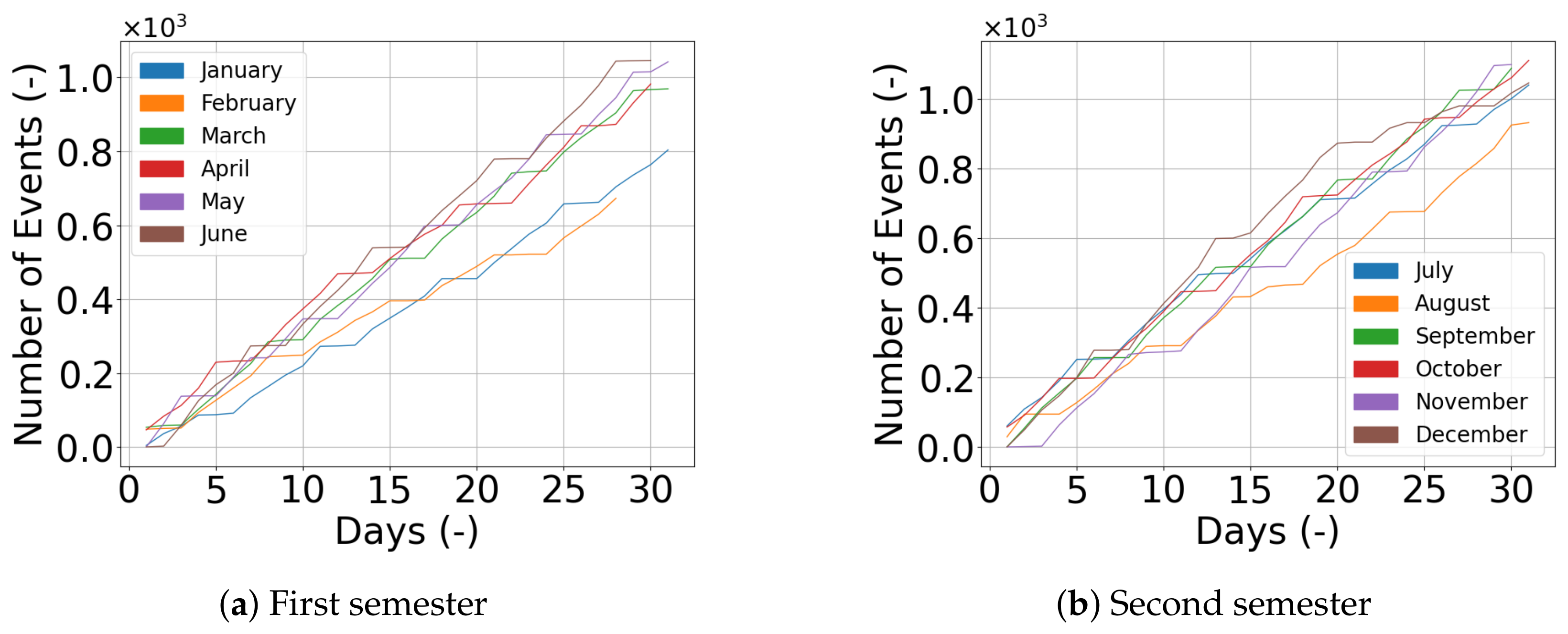
The proper use of Poisson processes requires the definition of a data framework and validation of a set of properties; these will be highlighted in the following section. An initial and foreseen step would be to classify the dataset in order to regroup behaviors reflecting similar average arrival rates. Categories could be temporal, like months, weeks, and days, or be based on other factors, like vehicle ID. As illustrated in Figure 4, the Poisson process path has different variations from one month to another, already highlighting a reason for interest in identifying trends from the initial yearly basis dataset.

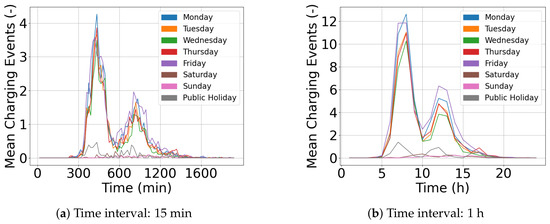
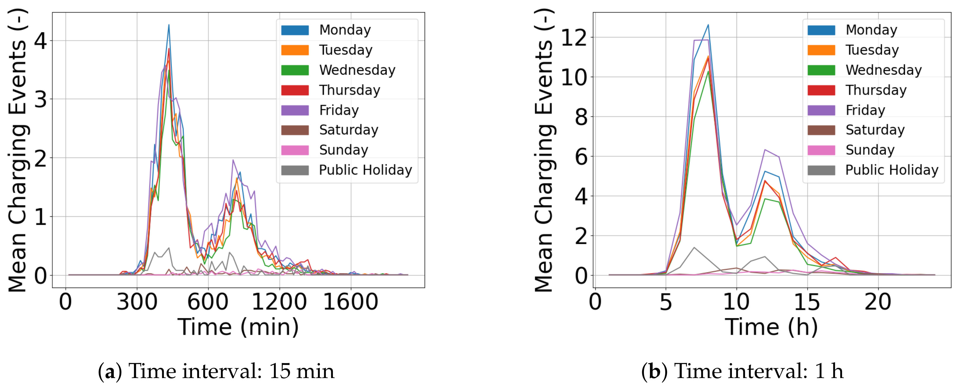
The observations also show that events fluctuate differently according to the day. Indeed, the arrival average profiles on weekdays, weekends, and public holidays sometimes have a comparable shape but with distinct amplitudes, as shown in Figure 5. One can observe two peaks of charging events on the different curves: one in the morning between 8 am and 9 am, the other one in the afternoon around 2 pm. The number of events during weekends is negligible, while days off demonstrate some signs of charging events and could belong to a different mode compared to weekdays. It should be noted that there are almost no charging events at night.

As already mentioned, modeling electric vehicle charging events based on cars’ ID clusters is another possibility. However, considering the number of electric vehicles composing the SAP fleet at Sophia Antipolis and the 11,863 associated charging events, this seems a complex a priori approach. A first interesting empirical classification of average intensity profiles would be to consider a clustering by day, like in Figure 5.

Another important step is to select the best representative and adapted time interval over which the number of rare events occurring will be counted. In a Poisson process framework, it is commonly accepted that the intensity $\lambda$, for a chosen interval, should correspond to a specific range of values, generally given in the literature as $3<\lambda <18$. As illustrated in Figure 5, an hourly interval seems to be an interesting compromise that respects the aforementioned condition for modeling the number of charging sessions. Additionally, it is also important to take into account that modeling stochastic intensities requires a representative distribution of events within the chosen time step for an optimal representation, as detailed in Section 3.2.2.

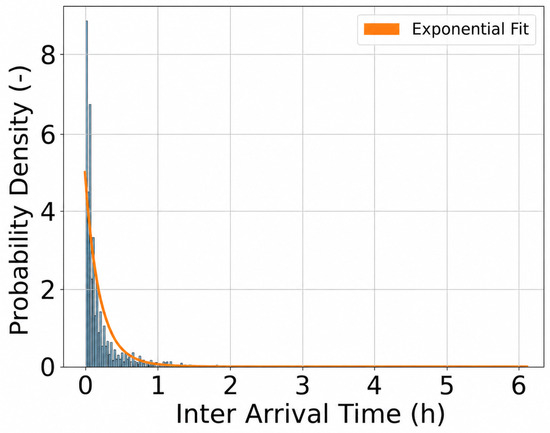
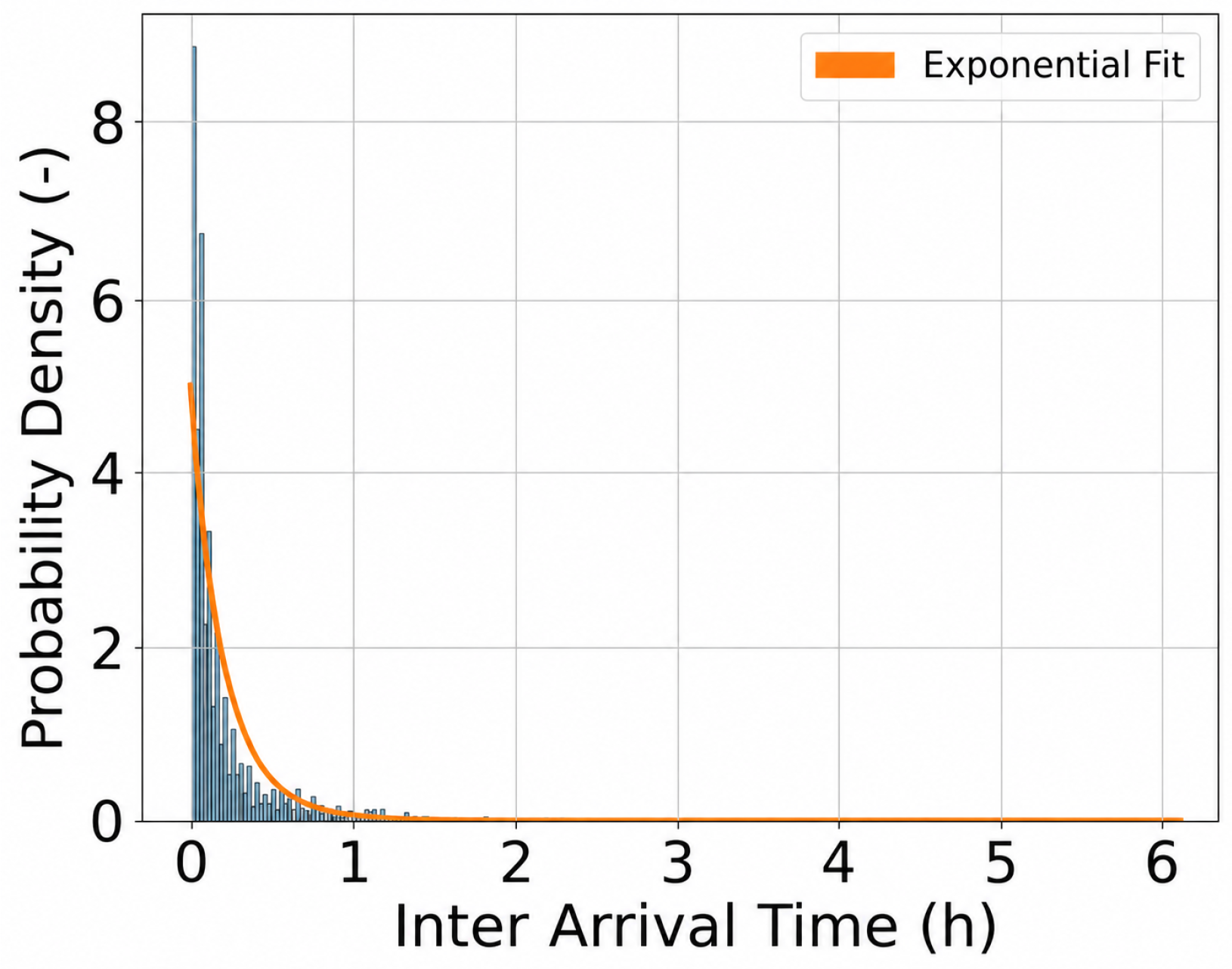
Advanced properties like the equality existing between the standard deviation and the mean of the counting process in Equation (1) or the inter-arrival time distribution in Equation (3) could also be considered to verify the compatibility between the studied dataset and Poisson processes requirements. As example, Figure 6 highlights the exponential distribution behavior of the inter-arrival times in 2019.

Once the dataset was prepared and organized, charging events were modeled as described in the following section.

3.2. Poisson Process Structures and Parameter Identification

3.2.1. Poisson Process Model Architectures

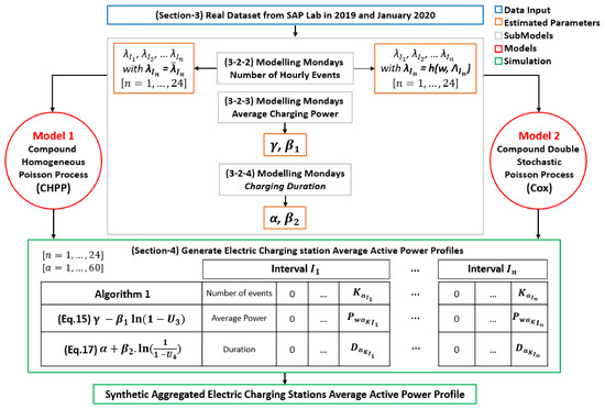
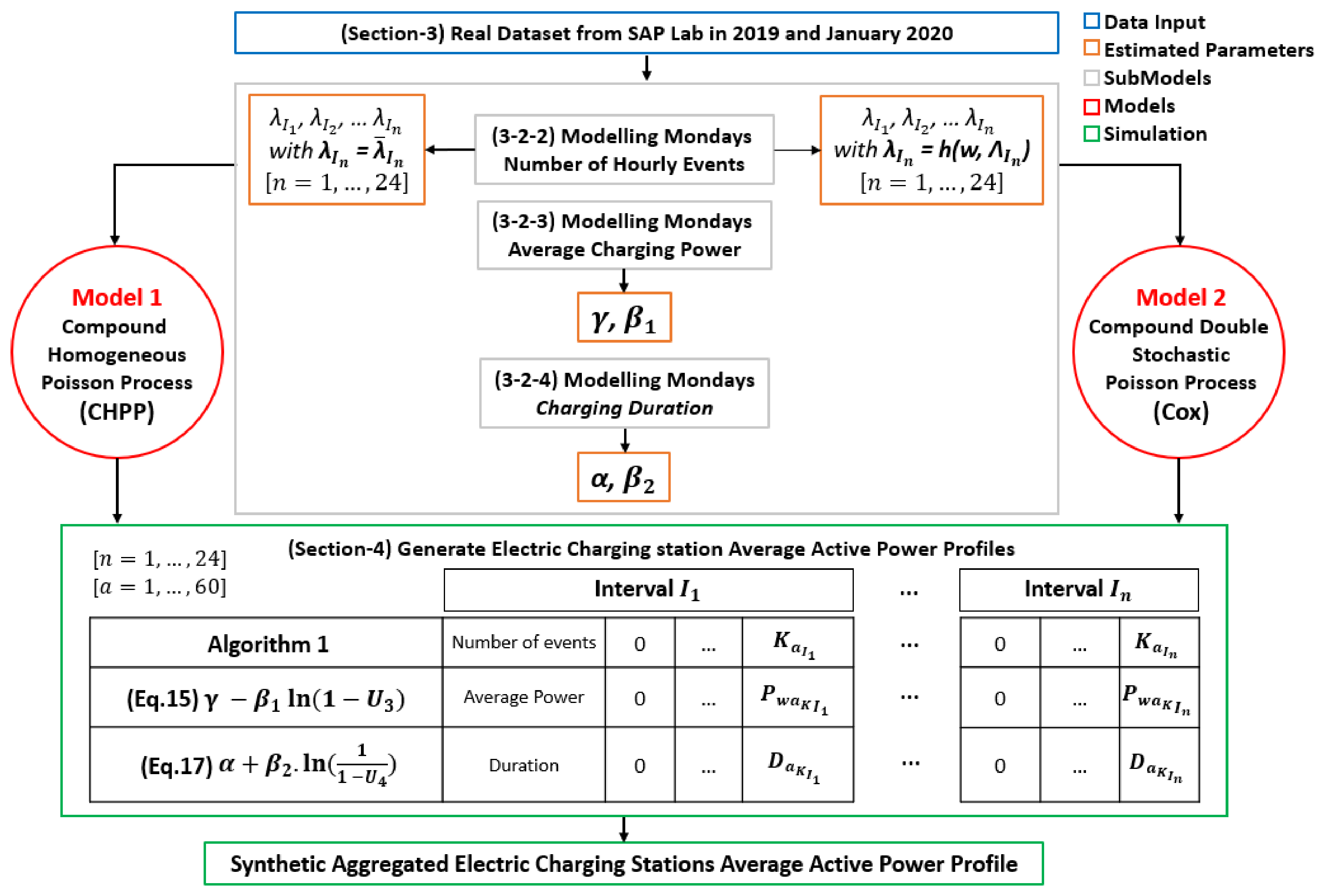
Two models, generating stochastic daily EVSE charging average power profiles, are detailed and compared. The first one is based on a compound homogeneous Poisson process and the second one is built on a double stochastic compound Poisson process; both models include the duration of events. Poisson processes can use a deterministic or a stochastic intensity ${\lambda }_{In}$ according to the architecture presented in Figure 7. The different parameters of the distributions are estimated with real arrival times, durations, and average powers from charging sessions occurring in 2019 at SAP Lab Sophia Antipolis. Two public holidays, considered as outliers, have been removed from the dataset. In Section 4, these models are implemented and compared. For each simulated day, with a chosen step time, a random number of events, with their respective random power and duration, are generated. Then, the charging profiles are aggregated to build a daily consumption pattern, allowing temporal or quantitative predictions, which will be discussed at the end.

Models 1 and 2, corresponding, respectively, to a homogeneous compound Poisson process with duration and a double stochastic compound Poisson process with duration, are implemented and compared in the next sections.

3.2.2. Modeling Daily Arrivals with Poisson Processes

Starting from the previous considerations in Section 2.2 and Section 2.3, daily arrival modeling can be approximated from two different perspectives: one based on the deterministic intensity and another considering the stochastic intensity. For instance, the SAP company, keeping track of the number of electric vehicle charging events each day at Sophia Antipolis, may notice that they have an average number ${\lambda }_{I_n}$ of k charges per interval of time $I_n$. If charging any particular vehicle does not affect the arrival time of future cars (there are incentives or enough charging stations to avoid congestion), and if cars arrive independently of one another, then a reasonable assumption is that the number of charging events per interval time follows a homogeneous Poisson distribution. The independence assumption constitutes a limitation of the proposed framework, since charging behaviors may exhibit temporal and social correlations in real-world environments. Based on an hourly interval $I_n$, with $n=1,2,\dots ,24$ representing the interval number, the probability mass function of events $\mathbb{P}(X_{I_n}=k)$ can be calculated by changing the intensity ${\lambda }_{I_n}$ every hour in Equation (10):

$$\mathbb{P}(X_{I_n}=k)={\displaystyle \frac{{\lambda }_{I_n}^k{e}^{-{\lambda }_{I_n}}}{k!}},\mathrm{with}{\lambda }_{I_n}\ge 0.$$

(10)

For the current homogeneous Poisson process, ${\lambda }_{I_n}$ represents the average value of charging events for a specific day in a one-hour time window during 2019.

Table 2. Average values of ${\lambda }_{I_n}$ between 5 a.m. ($I_6$) and 2 p.m. ($I_{14}$) on Mondays in 2019.

	${\overline{\lambda }}_{I_6}$	${\overline{\lambda }}_{I_7}$	${\overline{\lambda }}_{I_8}$	${\overline{\lambda }}_{I_9}$	${\overline{\lambda }}_{I_{10}}$	${\overline{\lambda }}_{I_{11}}$	${\overline{\lambda }}_{I_{12}}$	${\overline{\lambda }}_{I_{13}}$	${\overline{\lambda }}_{I_{14}}$
${\lambda }_{I_n}$ Monday	2.1	11.0	12.5	5.1	1.5	3.2	5.2	4.8	1.9

shows some ${\lambda }_{I_n}$ values for events occurring on Mondays.

The choice of a one-hour interval was made to better satisfy the assumptions of a homogeneous Poisson process, in particular ensuring $3<{\lambda }_{I_n}<18$. It can be noted that for some intervals in Table 2 the estimated values slightly exceed these bounds and may contribute to the overall model error.

The following Algorithm 1 can be used to generate a random number of $K_{I_n}$ hourly arrivals on the interval $I_n$ with ${\lambda }_{I_n}={\overline{\lambda }}_{I_n}$.

Algorithm 1 Generating Poisson-distributed Random Number of Events

Require:  ${\lambda }_{I_n}$ {Average rate of events per time unit} Ensure:  $K_{I_n}$ {Generated number of events on interval $I_n$}  1: $L_{I_n}\leftarrow e^{-{\lambda }_{I_n}}$ {Compute $L_{I_n}$}  2: $K_{I_n}\leftarrow 0$ {Initialize event counter on interval $I_n$}  3: $m\leftarrow 1$ {Initialize product of random numbers}  4: while $m>L_{I_n}$ do  5:    $K_{I_n}\leftarrow K_{I_n}+1$ {Increment event counter}  6:    $U_1\leftarrow \mathrm{Uniform}(0,1)$ {Generate a uniformly distributed random number}  7:    $m\leftarrow m\times U_1$ {Update the product}  8: end while  9: return $K_{I_n}-1$ {Return the generated number of events}

This pseudo-code generates Poisson-distributed random events $K_{I_n}$ by using the cumulative distribution function of the Poisson distribution and the properties of the exponential distribution. The threshold $L=e^{-{\lambda }_{I_n}}$ ensures that the product of uniform random variables simulates the cumulative probability of events in a Poisson process.

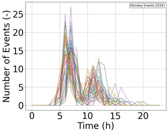
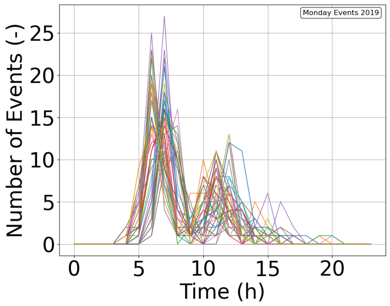
The homogeneous Poisson process is a simple way to model charging-event occurrences by taking an average intensity over a given period of time. But the average ${\lambda }_{I_n}$ in Table 2 is sometimes out of the boundaries of a Poisson process framework. Analyzing Figure 8, where events are represented for the same day over a complete year, it clearly appears that the values of the average intensity are not steady but depend both on the time of day and on the week, even if these days are all Mondays.

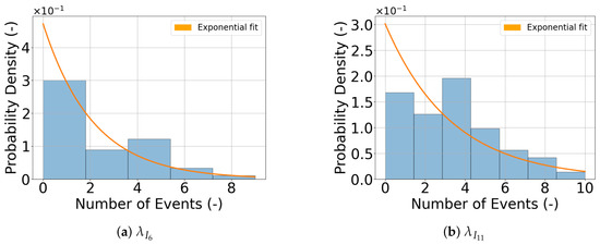
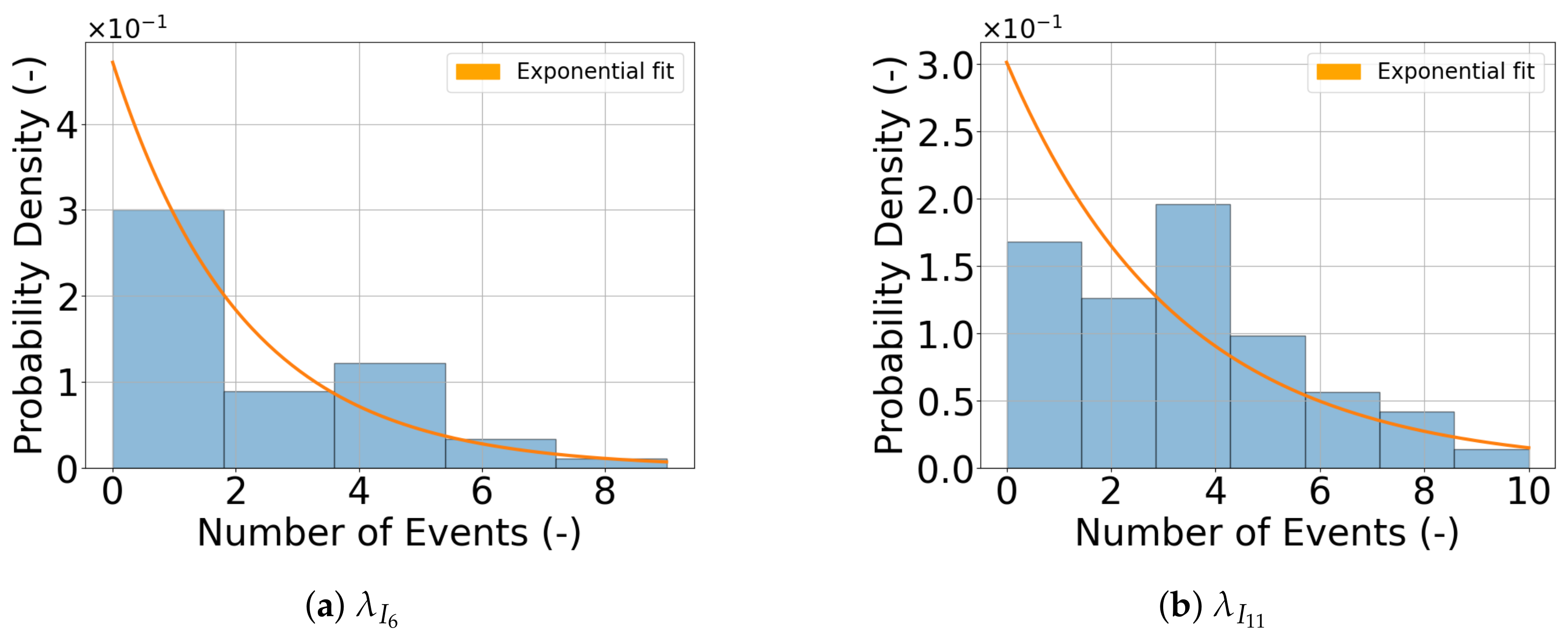
An extended and interesting approach in Figure 9 is then to consider that the intensity ${\lambda }_{I_n}$ is a random value, getting a specific distribution for each hour with a rate parameter ${\Lambda }_{I_n}$ when charging actions exist.

The double stochastic Poisson process can be expressed by Equation (11):

$$\mathbb{P}(X_{I_n}=k)={\displaystyle \frac{{\lambda }_{I_n}^k{e}^{-{\lambda }_{I_n}}}{k!}},\mathrm{with}{\lambda }_{I_n}=h(w,{\Lambda }_{I_n}),$$

(11)

where

$$h(w,{\Lambda }_{I_n})={\Lambda }_{I_n}{e}^{-{\Lambda }_{I_n}w}.$$

(12)

where w is the random variable representing the stochastic intensity and ${\Lambda }_{I_n}$ is the rate parameter of an exponential distribution.

Table 3. Example of values for ${\Lambda }_{I_n}$ between 5 a.m. and 2 p.m. on Mondays in 2019.

	${\Lambda }_{I_6}$	${\Lambda }_{I_7}$	${\Lambda }_{I_8}$	${\Lambda }_{I_9}$	${\Lambda }_{I_{10}}$	${\Lambda }_{I_{11}}$	${\Lambda }_{I_{12}}$	${\Lambda }_{I_{13}}$	${\Lambda }_{I_{14}}$
${\Lambda }_{I_n}$ Monday	0.47	0.10	0.11	0.19	0.64	0.30	0.18	0.25	0.52

shows some ${\Lambda }_{I_n}$ values for events on Mondays.

Like for the compound homogeneous Poisson process, Algorithm 1 can be used to generate a random number $K_{I_n}$ of hourly arrivals but with, in this specific case, ${\lambda }_{I_n}=h(w,{\Lambda }_{I_n})$, following Equation (13):

$${\lambda }_{I_n}=-{\Lambda }_{I_n}ln(1-U_2),$$

(13)

where ${\Lambda }_{I_n}$ is the rate parameter of an exponential distribution on the interval $I_n$ and $U_2$ is a randomly drawn number from a uniform distribution between 0 and 1.

Due to the random nature of ${\lambda }_{I_n}$, the double stochastic Poisson process, also known as the Cox process, should offer a better realistic vision of charging events rather than homogeneous modeling. Indeed, the Cox process provides some flexibility by allowing the intensity to not only depend on time but also to take arbitrary values due to a stochastic process.

3.2.3. Modeling Load Amplitude of EV Charging Events

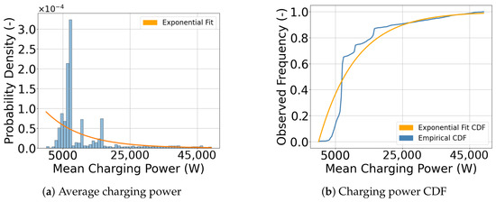
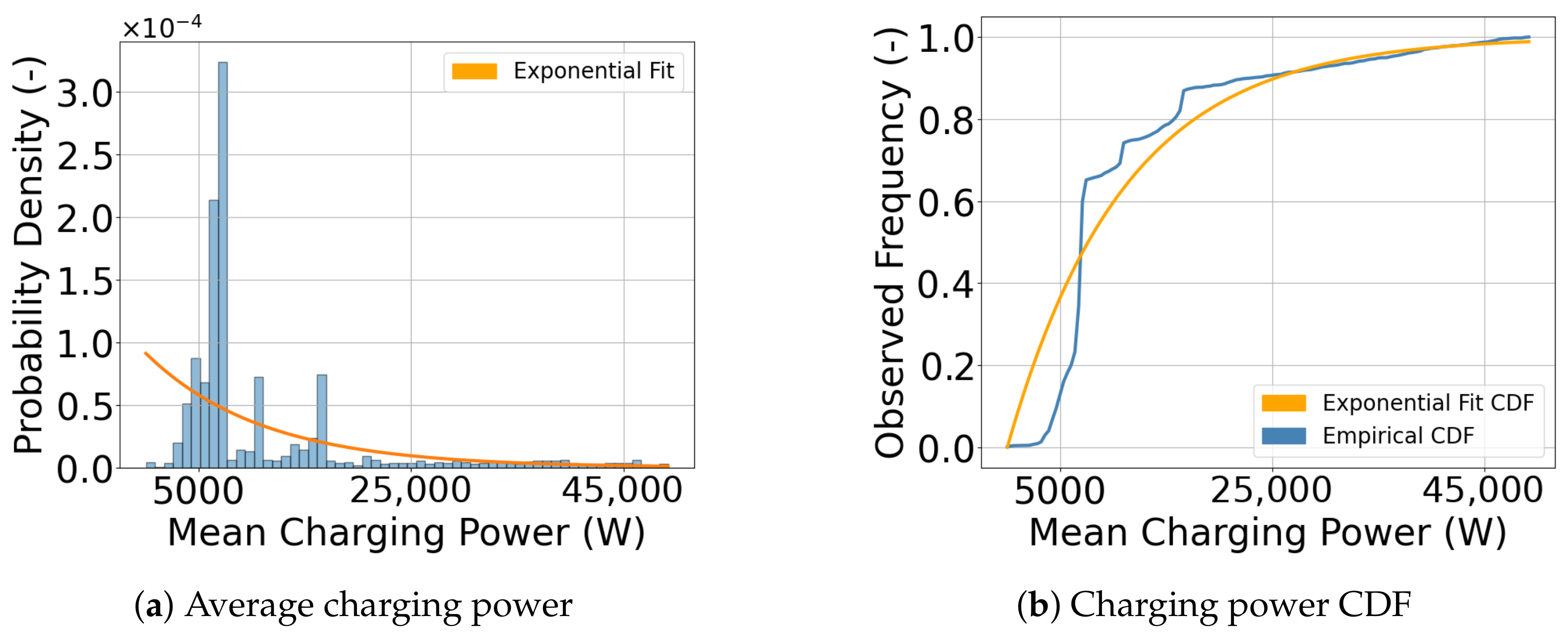
The aforementioned models can be upgraded using a compound Poisson process, as explained in Section 2.4, that also takes into account the average power that is withdrawn by cars during the charging period. As illustrated in Figure 10, the average active charging power distribution from the SAP dataset can be approximated by an exponential distribution. The fit and resulting parameters are computed by minimizing the negative log-likelihood function. This methodology is standard for estimating the parameters of compound Poisson processes other than the parameter $\Lambda$ of the intensity $\lambda$.

The exponential probability mass function can be expressed by Equation (14):

$$Exponential(y;{\beta }_1,\gamma )={\displaystyle \frac{1}{{\beta }_1}}{e}^{-{\displaystyle \frac{y-\gamma }{{\beta }_1}}},$$

(14)

where y is the random variable representing the average charging power during a charging session, ${\beta }_1$ is the scale parameter, and $\gamma$ is the location parameter. The optimal parameter values are ${\beta }_1$ = 10,970.48 (W) and $\gamma =60$ (W). The random average active charging power $P_w$ can be extracted from Equation (15):

$$P_w=\gamma -{\beta }_{1}ln(1-U_3),$$

(15)

where $\gamma$ is the location parameter, ${\beta }_1$ is the scale parameter, and $U_3$ is a random number drawn from a uniform distribution between 0 and 1.

The average charging power was quite challenging to model. Indeed, different distributions were tested, as shown in

Table 4. RMSE comparison between different distributions.

	Exponential	dWeibull	Gamma	Normal	Laplace	Logistic	Weibull
RMSE ($\times {10}^{-5}$)	4.34	2.41	5.14	4.29	3.40	3.78	4.00

, and a double Weibull fit was initially chosen.

Although the double Weibull distribution achieved a lower RMSE, the exponential distribution demonstrated significantly higher robustness during Monte Carlo simulations and avoided unstable extreme realizations during the forecasting process in Section 4.

3.2.4. Modeling the Duration of EV Charging Events

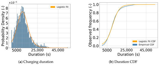
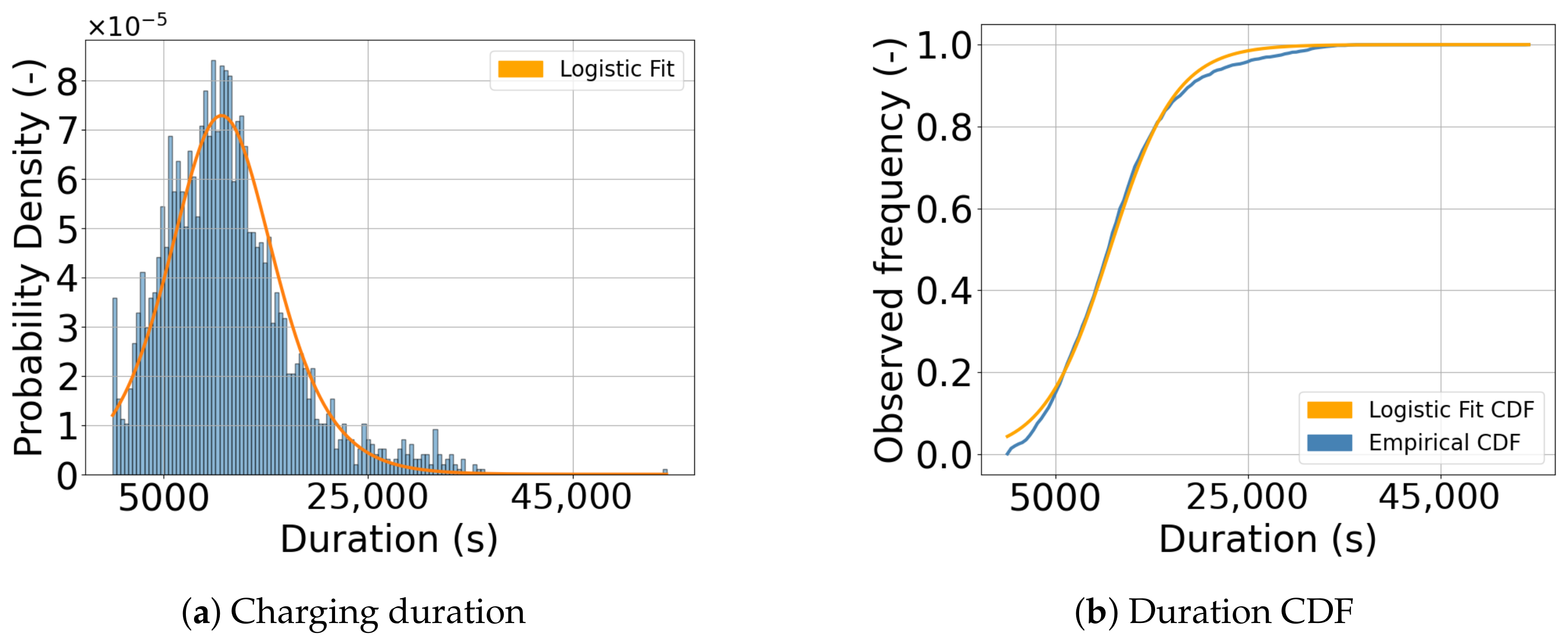
The last important step in the model architecture is to determine a distribution for the duration of charging sessions. As a reminder, in this article the duration only takes into account the charging phase, with an observed logistic distribution, as represented in Figure 11.

The logistic probability mass function can be expressed by Equation (16), and parameters of the distribution are, like in Section 3.2.3, estimated by minimizing the negative log-likelihood function:

$$Logistic(z,\alpha ,{\beta }_2)={\displaystyle \frac{e^{\frac{-(z-\alpha )}{{\beta }_2}}}{{\beta }_2{(1+e^{\frac{-(z-\alpha )}{{\beta }_2}})}^2}},ifz>0,$$

(16)

where z is the random variable representing the duration of the charging session, $\alpha$ is the mean of the logistic distribution, and ${\beta }_2$ is the scale parameter (or standard deviation) of the logistic distribution. The best-fit parameter values obtained from the maximum-likelihood process are $\alpha$ = 10,672.38 (s) and ${\beta }_2=3341.18$ (s).

Then, the random duration D of each charging event can be extracted from Equation (17):

$$D=\alpha +{\beta }_{2}ln\left({\displaystyle \frac{1}{1-U_4}}\right),$$

(17)

where $\alpha$ is the mean of the logistic distribution, ${\beta }_2$ is the scale parameter of the logistic distribution, and $U_4$ is a random number drawn from a uniform distribution between 0 and 1.

Combining the previous random average charging power and duration formulas in Section 3.2.3 and Section 3.2.4 with the random number of events in Section 3.2.2, models 1 an 2 can be expressed as a sequence of random events defined over the interval $I_n$ by Equation (18):

$${\mathcal{O}}_{I_n}={\left\{\left(P_w^{\left(i\right)},D^{\left(i\right)}\right)\right\}}_{i=1}^{X_{I_n}},\mathrm{where}{X}_{I_n}\sim \mathcal{P}\left({\lambda }_{I_n}\right)$$

(18)

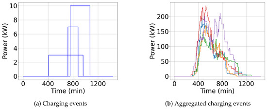
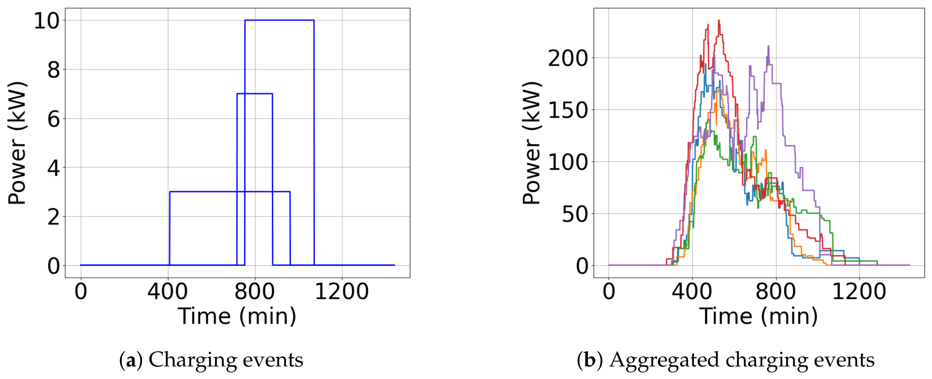
In other words, during the interval $I_n$, we observe $X_{I_n}$ events, each characterized by an amplitude $P_w^{\left(i\right)}$ and a duration $D^{\left(i\right)}$, for $i=1,\dots ,X_{I_n}$. It is then possible to simulate daily EVSE average active power profiles, as shown in Figure 12a, and the resulting daily aggregated consumption curves, shown in Figure 12.

4. Model Validation

4.1. Modeling EV Charging Events

An important goal of the validation process is to generate new charging curves, which will be called synthetic, from models with the architecture shown in Figure 7. However, the SAP Lab’s dataset was collected with a one-minute interval, whereas the ${\lambda }_{In}$ parameters are given on an hourly basis. To ensure a meaningful comparison between real and synthetic charging curves, a one-minute period is used to model Monday events based on models 1 and 2 using and combining Algorithm 1, and Equations (15) and (17). Then, $[K_{1_{I1}}$, …, $K_{{60}_{I1}}]$ … $[K_{1_{In}}$, …, $K_{{60}_{In}}]$, representing random events each minute on hourly intervals $I_n$ (with $n=1,2,...,24$), are considered independent and identically distributed following a Poisson distribution with parameter

$${\lambda }_{K_{a_{In}}}=\left({\displaystyle \frac{{\lambda }_{In}}{60}}\right),$$

(19)

where ${\lambda }_{In}$ is the hourly deterministic or stochastic intensity presented in Section 3.2.2 and $a=1,2,...,60$ is the index corresponding to each minute of an interval $I_n$.

Figure 12a shows an example of random individually generated average active power consumption profiles extracted from the two models. Then, Figure 12b shows the daily aggregated curves of these random profiles.

The representativeness of the simulated curves, compared to real data, is estimated in the next section.

4.2. Comparative Evaluation of Model Outcomes

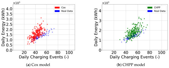
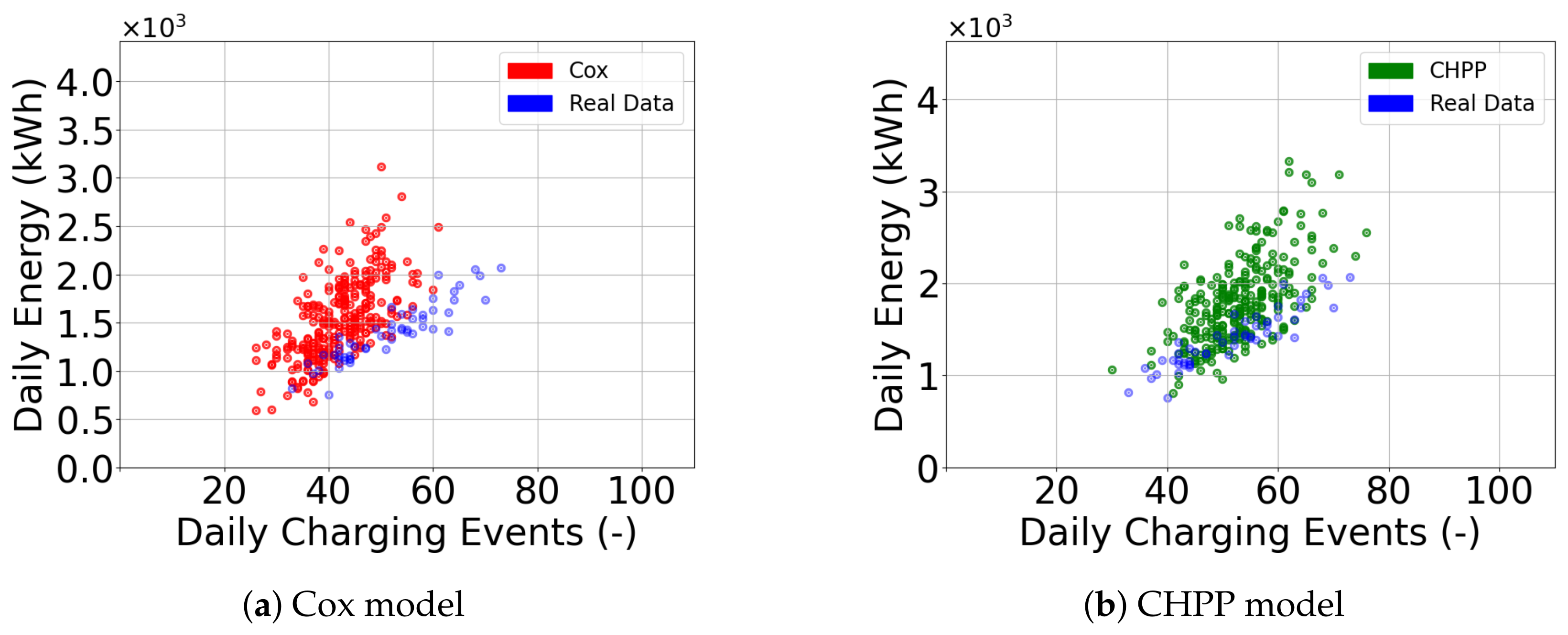
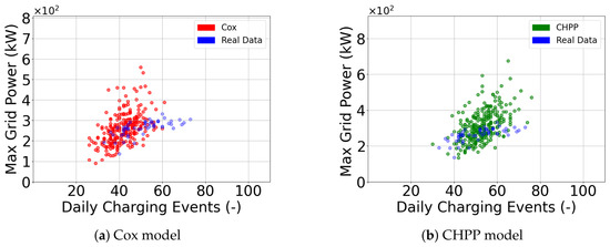
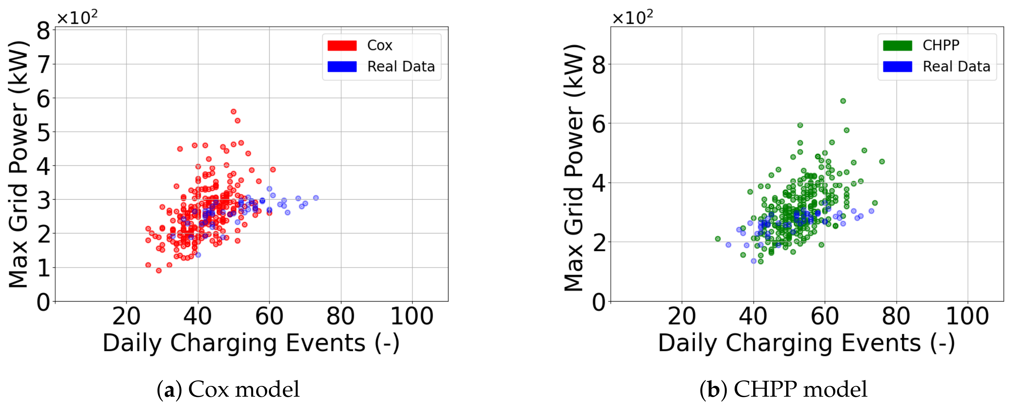
In order to compare both models, based on real-life situations and, in particular, field considerations, in addition to standard indicators, two criteria were selected for their operationality: The daily energy consumed during all daily charging sessions and the associated maximum power withdrawn from the grid were extracted from the real data and the synthetic curves. For each criterion, two hundred synthetic years, each containing 50 Monday charging events, were simulated and compared to 50 real Mondays from 2019 at SAP Lab Sophia Antipolis (two public holidays were removed). Note that in Figure 13 and Figure 14, only 250 points, equivalent to five synthetic years, and the 50 real Mondays are graphically visualized.

4.2.1. Daily Energy Consumed

Understanding daily energy demands could guide decisions on charging station locations, capacities, and user experience, contributing to efficient grid management, cost-effective operations, and fostering a comprehensive and balanced growth in the electric mobility sector.

The results for the daily energy consumed from the two models are illustrated in Figure 13.

Both models tend to overestimate daily energy, likely due to cumulative errors in power, duration, and occurrence. Improving each component could reduce the overall error.

4.2.2. Maximum Grid Power Demand

Like the daily energy demand, modeling the maximum grid power extracted by electric vehicle charging stations is also crucial for efficient grid planning, infrastructure scaling, and load balancing. This knowledge could help in grid resilience, enables smart grid implementation, and supports cost-effective measures in the evolving landscape of electric mobility.

The maximum grid power demand resulting from the two models is illustrated in Figure 14.

The simulated point clouds in Figure 13 and Figure 14 appear quite comparable to real data point clouds, showing no significant outliers. A first overview of the precision and the volatility of the two models is presented in

Table 5. Daily energy consumption statistics for real data and predictions.

Daily Energy Consumed	Average	Median	Std
Real data (kWh)	1369	1376	285
CHPP (kWh)	1667	1636	393
$\Delta$ Real/CHPP (%)	21.8	18.9	37.9
Cox (kWh)	1454	1423	377
$\Delta$ Real/Cox (%)	6.2	3.4	32.4

and

Table 6. Maximum daily grid power statistics for real data and predictions.

Maximum Daily Grid Power	Average	Median	Std
Real data (kW)	263	268	37
CHPP (kW)	288	281	75
$\Delta$ Real/CHPP (%)	9.6	4.8	101
Cox (kW)	247	240	70
$\Delta$ Real/Cox (%)	5.8	10.4	87.1

. Although the data cannot be fit by a normal law, the standard deviation of errors is provided, as there is a large amount of simulated data.

Overall, both models capture the global statistical trends in EV charging demand, although significant variability remains at the daily scale, especially in peak power estimation, along with volatility measures that are sufficient for operational decision making. As expected, the Cox model performs slightly better than the CHPP model, with a modeling accuracy of 6.2% for the energy and 5.8% for the power. The next subsection shows the forecasting capability of these models with respect to the amount of data used for parameter estimation.

4.2.3. Daily Electric Vehicles Charging Stations Average Power Profile Forecast

After identifying the double stochastic compound Poisson process as the most promising candidate, it is possible to use the methodology presented in this article as a forecasting approach, where models are tuned on the whole dataset available up to a certain date in order to forecast the following day, like in [31].

The key benefit of the model is that parameter estimation can be updated and improved when new real data are available. The idea is to test to what extent this update is significant by analyzing the accuracy, the robustness, and the capacity of the model to generate a broad diversity of profiles with respect to the number of data used for the parameter estimation. To achieve this, Monday forecasts are performed over three different time windows, more precisely, in March 2019, October 2019, and January 2020. For each time window, only the data during the months before the prediction (starting from January 2019) are used to calibrate the model, that is, only eight Mondays for the first forecast in March 2019, and up to fifty-three Mondays for the last one at the end of January 2020. To sum up, the current framework follows a rolling-horizon forecast with a fixed starting point in January 2019. Calibration was realized using the real dataset from SAP Lab at Sophia Antipolis, where charging events were registered with an average charging power ranging from 3 kW to 46 kW. For each forecast, 10,000 synthetic Monday EVSE charging events were simulated.

In order to evaluate the generative models beyond average accuracy, we propose a composite score that balances the precision of simulations and the ability to generate a high variety of profiles. Let $x_{a,n}^{\mathrm{real}}$ be the real observed value at minute a of hour n, and let $x_{a,n}^{\left(j\right)}$ be the corresponding value in the j-th simulated profile. The average simulated value at each point is denoted by ${\overline{x}}_{a,n}^{\mathrm{fc}}$. We introduce the following:

• The mean absolute error between the real profile and the average of the simulated profiles:

  $${\mathrm{MAE}}_{\mathrm{rs}}={\displaystyle \frac{1}{24\times 60}}{\displaystyle \sum _{n=1}^{24}}{\displaystyle \sum _{a=1}^{60}}\left|x_{a,n}^{\mathrm{real}}-{\overline{x}}_{a,n}^{\mathrm{fc}}\right|$$

  (20)
• The average intra-group deviation of each simulated profile from the simulated mean:

  $${\mathrm{MAE}}_{\mathrm{igs}}={\displaystyle \frac{1}{N}}{\displaystyle \sum _{j=1}^N}\left({\displaystyle \frac{1}{24\times 60}}{\displaystyle \sum _{n=1}^{24}}{\displaystyle \sum _{a=1}^{60}}\left|x_{a,n}^{\left(j\right)}-{\overline{x}}_{a,n}^{\mathrm{fc}}\right|\right)$$

  (21)
• A composite score evaluating the diversity of the profiles vs. forecast accuracy:

  $$\mathrm{Score}={\displaystyle \frac{{\mathrm{MAE}}_{\mathrm{igs}}}{{\mathrm{MAE}}_{\mathrm{rs}}}}$$

  (22)

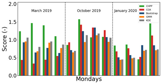
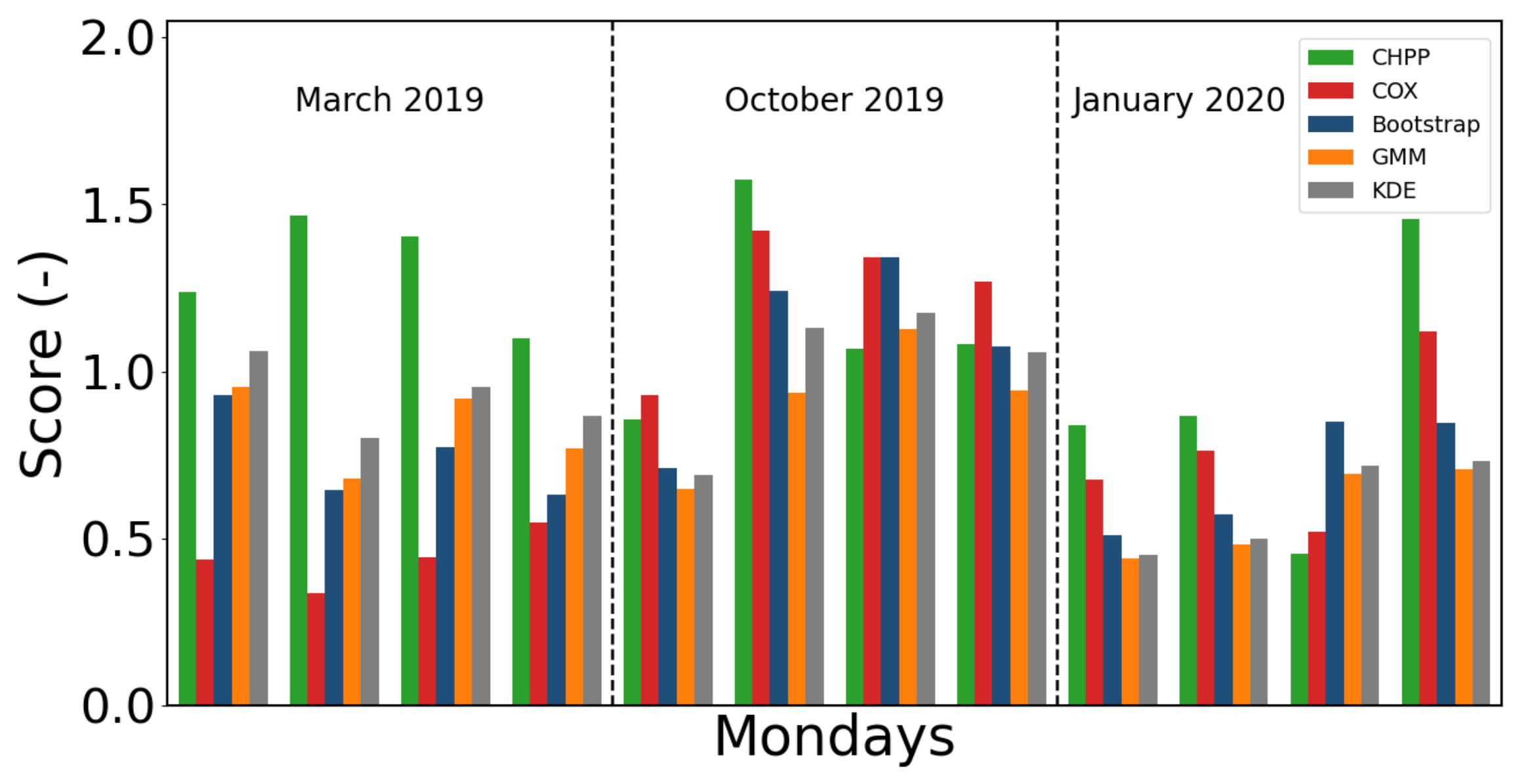
This score promotes models that not only match the real data on average with a low fidelity error, but also generate a realistic and diverse set of profiles, which is critical for applications such as flexibility forecasting or volatility quantification in energy systems, as shown in Figure 15.

Figure 15 shows the forecast scores for Mondays in March, October, and then the following January. Each time, the model is calibrated and parameters updated with the data from the previous months. When the models have been calibrated with a small amount of data, the compound homogeneous Poisson process is superior to the compound Cox process, but the performance difference tends to decrease when more data are available.

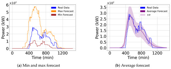
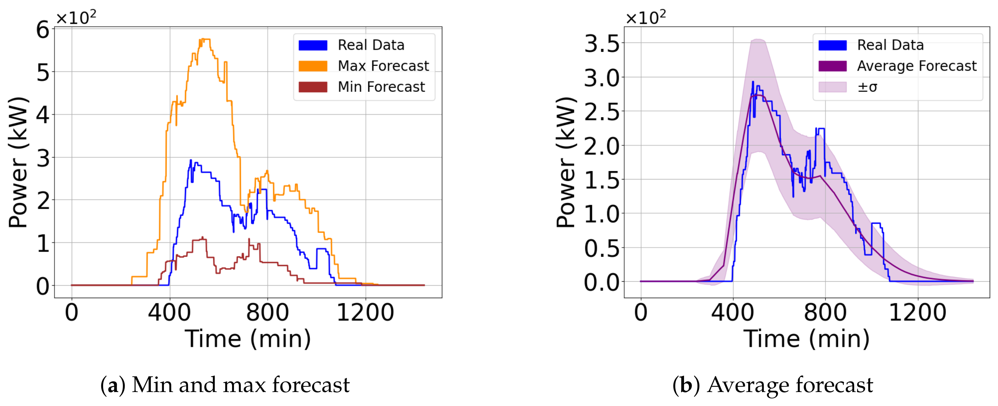
Let us focus on the last prediction, Monday 27/01/2020, using the compound homogeneous Poisson process that has the best score for this specific day. The maximum, minimum, and average power profiles of the 10,000 synthetic (generated) curves are represented in Figure 16a every minute with the real aggregated EVSE consumption curve, and the average forecast is shown in Figure 16b.

As illustrated by Figure 16b, the average curve of the forecast aggregated daily consumption charging sessions is quite similar to the real Monday consumption profile and provides a representative estimation of the real events with a mean absolute error equal to 15.2 kW, representing 5.1% of the maximum power withdrawn from the grid on 27/01/2020.

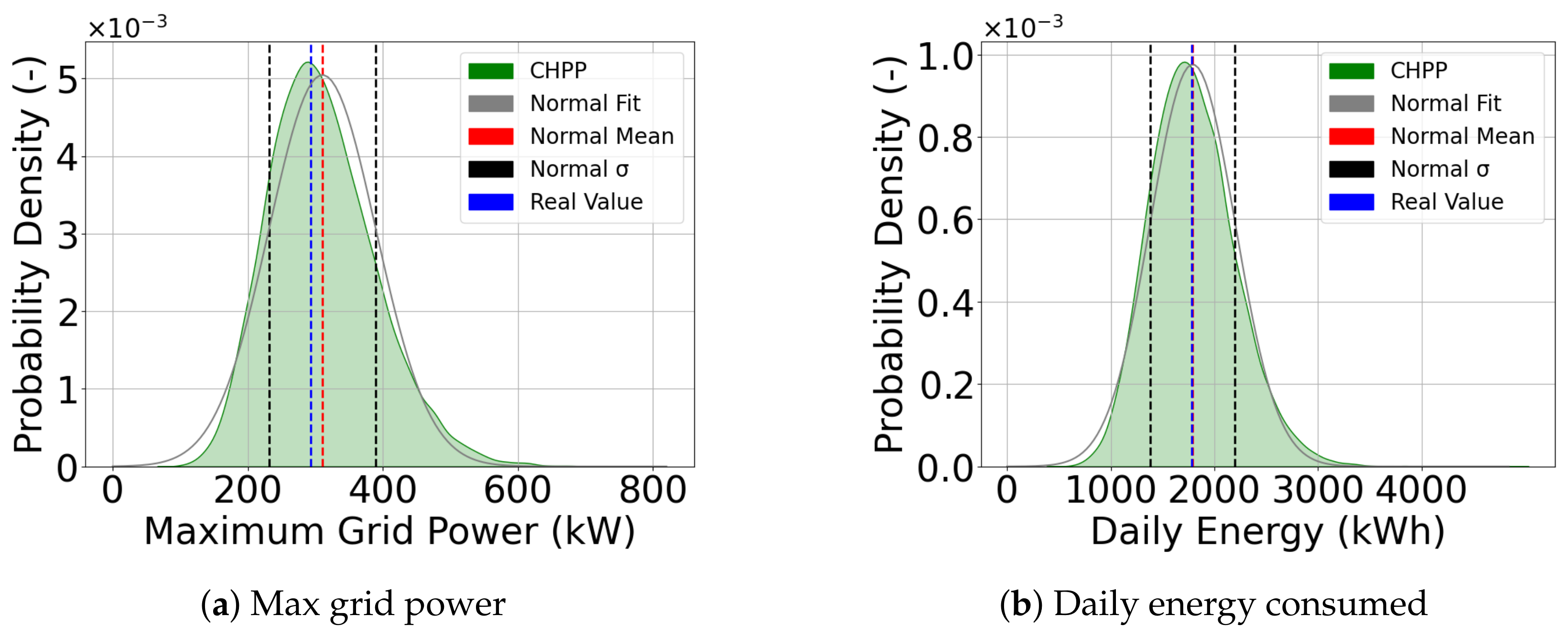
Beyond the previous temporal prediction, it is also possible to realize a quantitative forecast using the indicators given in Section 4.2.1 and Section 4.2.2: the daily energy consumed during all charging sessions and the associated maximum power withdrawn from the grid. The density distributions of the 10,000 synthetic Mondays in Figure 17 can be fitted with a normal law, providing an overview of the forecast volatility and therefore of the robustness of the method.

Based on the normal distribution fit in Figure 17, the real values of daily energy consumed and maximum power demand are found to be close to the mean of the forecast distributions, yielding average errors of 0.8% and 6.2%, respectively, for maximum grid power demand and daily energy consumption. In all cases, the real values remain within the interval $[\mu -\sigma ;\mu +\sigma ]$, containing 68.3% of the generated synthetic realizations. While this study only considers 1863 events, the methodology can be extended to larger datasets, as long as the Poisson assumption $3<\lambda <18$ holds, which is determined by the selected time interval. Advanced properties, like the equality existing between the standard deviation and the mean of the counting process in Equation (1) or the inter-arrival time distribution in Equation (3), could also be verified, as already highlighted in Figure 6. For larger and more heterogeneous datasets, hybrid approaches combining stochastic modeling and machine learning techniques could constitute promising research directions. It was shown in [32] that Poisson models could provide a good estimate to initialize such algorithms as recurrent networks. A good initialization of these networks is very important to ensure their convergence.

Finally, the proposed methodology provides a realistic probabilistic representation of aggregated EV charging demand while maintaining limited computational complexity and interpretable stochastic parameters.

4.2.4. Comparison with Existing Forecasting Approaches

Because forecasting objectives, datasets, charging infrastructures, and evaluation methodologies differ significantly across the literature, direct quantitative comparison with previously published EV charging forecasting studies remains difficult. Nevertheless, in order to provide a quantitative benchmark of the proposed methodology, three representative baseline approaches were implemented using the same historical dataset and forecasting protocol: Bootstrap resampling, Gaussian mixture models (GMMs), and kernel density estimation (KDE).

The bootstrap approach consists of randomly resampling complete historical daily charging profiles from the training dataset. The GMM baseline models the joint probability distribution of charging event characteristics, namely, arrival time, charging duration, and charging power, using a mixture of Gaussian distributions. The KDE approach provides a non-parametric estimation of the same joint distribution using Gaussian kernels. For each method, 10,000 synthetic daily charging profiles were generated and evaluated using the same performance indicators as those adopted for the proposed CHPP and Cox frameworks.

In addition to the quantitative benchmark,

Table 7. Qualitative comparison between representative EV charging forecasting approaches.

Method	Forecasting Accuracy	Interpretability	Computational Cost	Synthetic Profile Generation
Deep learning (LSTM/RNN)	High	Low	High	Limited
Gradient boosting/XGBoost	Medium–High	Medium	Medium	Limited
Gaussian mixture models	Medium	High	Low	Moderate
Kernel density estimation	Medium	High	Medium	Moderate
Hawkes processes	Medium	Medium	Medium–High	Moderate
Proposed CHPP/Cox framework	Medium	High	Low	Strong

provides a qualitative positioning of representative EV charging forecasting approaches commonly reported in the literature with respect to forecasting accuracy, interpretability, computational requirements, and synthetic profile generation capabilities.

Machine learning approaches may provide superior deterministic point-wise forecasting accuracy in some situations; however, they generally require significantly larger datasets, extensive hyperparameter tuning, and higher computational resources. Conversely, stochastic and statistical generative approaches are particularly attractive when the objective is to reproduce charging demand variability and generate realistic synthetic charging profiles for probabilistic analyses.

Table 8. Quantitative comparison of forecasting approaches. All reported metrics correspond to average values obtained over the twelve forecasting days presented in Figure 15.

Method	Avg. MAErs (kW)	Avg. MAEigs (kW)	Avg. Score	Avg. Energy Error (%)	Avg. Max Power Error (%)
Bootstrap	18.8	14.6	0.84	16.8	14.1
GMM	21.5	15.2	0.78	16.5	23.5
KDE	19.7	15.0	0.85	16.6	18.0
CHPP	22.5	22.1	1.12	14.5	10.9
Cox	27.2	19.6	0.82	27.8	26.6

summarizes the quantitative benchmark results obtained for all the considered forecasting approaches. For each method, the forecasting procedure was repeated on the twelve test days presented in Figure 15. All the reported metrics, including MAE_rs, MAE_igs, score, daily energy error, and maximum grid power error, correspond to average values computed over the twelve forecasting experiments.

The quantitative results indicate that bootstrap and KDE achieve slightly lower profile reconstruction errors (MAE_rs), whereas the proposed CHPP framework provides the lowest prediction errors for daily energy consumption and maximum grid power demand. Furthermore, CHPP achieves the highest score, reflecting an improved capability to reproduce the intrinsic variability of EV charging demand while maintaining satisfactory forecasting accuracy.

These results suggest that the proposed framework does not primarily aim at maximizing deterministic profile reconstruction accuracy. Instead, it provides a favorable compromise between forecast fidelity, synthetic profile diversity, and computational simplicity. Such characteristics are particularly relevant for applications including synthetic load profile generation, probabilistic grid impact assessment, flexibility studies, and Monte Carlo-based power system simulations.

4.3. Discussion and Perspectives

Several limitations of the proposed framework should nevertheless be acknowledged. First, the current methodology assumes statistical independence between charging events, whereas real EV charging behaviors may exhibit temporal correlations between users and charging sessions. Second, the proposed framework assumes sufficient charging infrastructure availability in order to neglect queuing and congestion effects. Consequently, the methodology is particularly well adapted to tertiary buildings or charging infrastructures where waiting times remain limited.

In addition, although the Cox process introduces stochastic variability in charging arrivals, more advanced self-exciting stochastic processes, such as Hawkes processes, could potentially better capture temporal dependencies between charging events.

Future work should therefore investigate user clustering techniques, temporal behavioral segmentation, charging congestion effects, and hybrid stochastic-learning approaches in order to improve forecasting accuracy and better represent heterogeneous EV charging behaviors. Hardware-in-the-loop validation and real-time implementation studies could also constitute valuable perspectives for future developments.

5. Conclusions

Two stochastic Poisson-based frameworks were investigated to model the daily power profile of EV charging stations and the stochastic variability of EV charging behavior using 1863 charging events recorded at a one-minute resolution from thirty-four 22 kW, two 50 kW, and one 150 kW charging stations. The proposed methodology can be employed as a forecasting tool by calibrating the stochastic model using historical charging data in order to predict future EV charging demand. Both stochastic models demonstrated satisfactory forecasting capabilities, with moderate performance differences depending on whether temporal or quantitative indicators were considered. Operationally relevant indicators, such as maximum grid power demand and daily energy consumption, were predicted, with average errors of up to 6.2% and 0.8%, respectively. In addition, the proposed frameworks were able to generate realistic and diversified synthetic charging profiles, which is particularly relevant for probabilistic power system studies and Monte Carlo-based simulations. Compared with highly data-intensive machine learning approaches, the proposed methodology relies on interpretable probabilistic parameters and limited computational resources, making it suitable for exploratory analyses and situations involving limited historical datasets. The proposed framework may therefore constitute a complementary stochastic modeling approach for EV charging demand forecasting, synthetic profile generation, and flexibility assessment in increasingly electrified distribution systems. Future work should investigate clustering techniques and user-dependent behavioral representations in order to improve forecasting accuracy and better capture temporal charging patterns and user heterogeneity. Additional extensions could also include the integration of self-exciting stochastic processes, such as Hawkes processes, or the consideration of charging infrastructure congestion effects. Overall, the results demonstrate that compound Poisson processes provide a flexible and computationally efficient framework for modeling EV charging demand and generating stochastic charging profiles for future smart grid and smart city applications, and probably beyond.

References

- RTE. Integration of Electric Vehicles into the Power System in France, 2019. Available online: https://assets.rte-france.com/prod/public/2020-09/RTE%20electromobility%20report.pdf (accessed on 24 June 2026).
- Gonzalez Venegas, F.; Petit, M.; Perez, Y. Active Integration of Electric Vehicles into Distribution Grids: Barriers and Frameworks for Flexibility Services. Renew. Sustain. Energy Rev. 2021, 145, 111060. [Google Scholar] [CrossRef] [Scilit]
- Rauma, K.; Funke, A.; Simolin, T.; Järventausta, P.; Rehtanz, C. Electric Vehicles as a Flexibility Provider: Optimal Charging Schedules to Improve the Quality of Charging Service. Electricity 2021, 2, 225–243. [Google Scholar] [CrossRef] [Scilit]
- Hasan, K.N.; Muttaqi, K.M.; Borboa, P.; Scira, J.; Zhang, Z.; Leishman, M. Distribution network voltage analysis with data-driven electric vehicle load profiles. Sustain. Energy Grids Netw. 2023, 36, 101216. [Google Scholar] [CrossRef] [Scilit]
- Rawat, T.; Singh, J.; Pandey, V.C.; Sharma, S. Planning renewables in distribution system with electric vehicles to improve hosting capacity and energy losses: Two-stage stochastic optimization framework. Sustain. Energy Grids Netw. 2024, 39, 101445. [Google Scholar] [CrossRef] [Scilit]
- Guzel, I.; Gol, M. Plug-in electric vehicle load modeling for charging scheduling strategies in microgrids. Sustain. Energy Grids Netw. 2022, 32, 100819. [Google Scholar] [CrossRef] [Scilit]
- Fuels Institute. EV Consumer Behavior; Ricardo Inc.: Van Buren Township, MI, USA, 2021. [Google Scholar]
- Li, S.; Xiong, H.; Chen, Y. DiffPLF: A Conditional Diffusion Model for Probabilistic Forecasting of EV Charging Load. Electr. Power Syst. Res. 2024, 235, 110723. [Google Scholar] [CrossRef] [Scilit]
- Jia, M.; Yang, B. EVformer: A Spatio-Temporal Decoupled Transformer for Citywide EV Charging Load Forecasting. World Electr. Veh. J. 2026, 17, 71. [Google Scholar] [CrossRef] [Scilit]
- Ostermann, A.; Haug, T. Probabilistic Forecast of Electric Vehicle Charging Demand: Analysis of Different Aggregation Levels and Energy Procurement. Energy Inform. 2024, 7, 13. [Google Scholar] [CrossRef] [Scilit]
- Zheng, K.; Xu, H.; Long, Z.; Wang, Y.; Chen, Q. Coherent Hierarchical Probabilistic Forecasting of Electric Vehicle Charging Demand. arXiv 2024, arXiv:2411.00337. [Google Scholar]
- Wang, Y.; Zhao, X.; Li, P. Modeling Electric Vehicle Charging Demand Using Self-Exciting Point Processes. Appl. Energy 2023, 344, 121231. [Google Scholar] [CrossRef] [Scilit]
- Chen, R.; Sun, H.; Zhang, W. Hybrid Probabilistic Deep Learning Framework for Electric Vehicle Charging Load Forecasting. IEEE Trans. Smart Grid 2024, 15, 1458–1470. [Google Scholar]
- Amara-Ouali, Y.; Goude, Y.; Massart, P.; Poggi, J.M.; Yan, H. A Review of Electric Vehicle Load Open Data and Models. Energies 2021, 14, 2233. [Google Scholar] [CrossRef] [Scilit]
- Rashid, M.; Elfouly, T.; Chen, N. A Comprehensive Survey of Electric Vehicle Charging Demand Forecasting Techniques. IEEE Open J. Veh. Technol. 2024, 5, 1348–1373. [Google Scholar] [CrossRef] [Scilit]
- Chung, Y.W.; Khaki, B.; Li, T.; Chu, C.; Gadh, R. Ensemble Machine Learning-Based Algorithm for Electric Vehicle User Behavior Prediction. Appl. Energy 2019, 254, 113732. [Google Scholar] [CrossRef] [Scilit]
- Zhang, X.; Zhang, Z.; Liu, Y.; Xu, Z.; Qu, X. A Review of Machine Learning Approaches for Electric Vehicle Energy Consumption Modelling in Urban Transportation. Renew. Energy 2024, 234, 121243. [Google Scholar] [CrossRef] [Scilit]
- Zhu, J.; Yang, Z.; Mourshed, M.; Guo, Y.; Zhou, Y.; Chang, Y.; Wei, Y.; Feng, S. Electric Vehicle Charging Load Forecasting: A Comparative Study of Deep Learning Approaches. Energies 2019, 12, 2692. [Google Scholar] [CrossRef] [Scilit]
- Metais, M.; Jouini, O.; Perez, Y.; Berrada, J.; Suomalainen, E. Too Much or Not Enough? Planning Electric Vehicle Charging Infrastructure: A Review of Modeling Options. Renew. Sustain. Energy Rev. 2022, 153, 111719. [Google Scholar] [CrossRef] [Scilit]
- Kumar, N.; Kumar, T.; Nema, S.; Thakur, T. A Comprehensive Planning Framework for Electric Vehicles Fast Charging Station Assisted by Solar and Battery Based on Queueing Theory and Non-Dominated Sorting Genetic Algorithm-II in a Co-Ordinated Transportation and Power Network. J. Energy Storage 2022, 49, 104180. [Google Scholar] [CrossRef] [Scilit]
- Khoo, Y.B.; Wang, C.H.; Paevere, P.; Higgins, A. Statistical Modeling of Electric Vehicle Electricity Consumption in the Victorian EV Trial, Australia. Transp. Res. Part Transp. Environ. 2014, 32, 263–277. [Google Scholar] [CrossRef] [Scilit]
- Flammini, M.G.; Prettico, G.; Julea, A.; Fulli, G.; Mazza, A.; Chicco, G. Statistical Characterisation of the Real Transaction Data Gathered from Electric Vehicle Charging Stations. Electr. Power Syst. Res. 2019, 166, 136–150. [Google Scholar] [CrossRef] [Scilit]
- Lee, Z.J.; Li, T.; Low, S.H. ACN-Data: Analysis and Applications of an Open EV Charging Dataset. In Proceedings of the Tenth ACM International Conference on Future Energy Systems; Association for Computing Machinery: New York, NY, USA, 2019; pp. 139–149. [Google Scholar] [CrossRef] [Scilit]
- Helmus, J.R.; Lees, M.H.; Van Den Hoed, R. A Data Driven Typology of Electric Vehicle User Types and Charging Sessions. Transp. Res. Part Emerg. Technol. 2020, 115, 102637. [Google Scholar] [CrossRef] [Scilit]
- Lahariya, M.; Benoit, D.; Develder, C. Defining a Synthetic Data Generator for Realistic Electric Vehicle Charging Sessions. In Proceedings of the Eleventh ACM International Conference on Future Energy Systems; Association for Computing Machinery: New York, NY, USA, 2020; pp. 406–407. [Google Scholar] [CrossRef] [Scilit]
- Wong, W.C.; Chung, C.Y.; Chan, K.W.; Chen, H. Quasi-Monte Carlo Based Probabilistic Small Signal Stability Analysis for Power Systems With Plug-In Electric Vehicle and Wind Power Integration. IEEE Trans. Power Syst. 2013, 28, 3335–3343. [Google Scholar] [CrossRef] [Scilit]
- Bremermann, L.E.; Matos, M.; Lopes, J.A.P.; Rosa, M. Electric Vehicle Models for Evaluating the Security of Supply. Electr. Power Syst. Res. 2014, 111, 32–39. [Google Scholar] [CrossRef] [Scilit]
- Ivarsoy, E.; Torsater, B.N.; Korpas, M. Stochastic Load Modeling of High-Power Electric Vehicle Charging—A Norwegian Case Study. In Proceedings of the 2020 International Conference on Smart Energy Systems and Technologies (SEST); IEEE: New York, NY, USA, 2020; pp. 1–6. [Google Scholar] [CrossRef] [Scilit]
- Khalkhali, H.; Hosseinian, S.H. Multi-Class EV Charging and Performance-Based Regulation Service in a Residential Smart Parking Lot. Sustain. Energy Grids Netw. 2020, 22, 100354. [Google Scholar] [CrossRef] [Scilit]
- Kutoyants, Y.A. Introduction to the Statistics of Poisson Processes and Applications; Springer Nature: Berlin/Heidelberg, Germany, 2023. [Google Scholar]
- Amara-Ouali, Y.; Goude, Y.; Poggi, J.M. Modelling the Intensity of Electric Vehicle Arrivals at Charging Points. Transp. Res. Procedia 2023, 70, 372–379. [Google Scholar] [CrossRef] [Scilit]
- Chacón, H.; Koppisetti, V.; Hardage, D.; Choo, K.K.R.; Rad, P. Forecasting call center arrivals using temporal memory networks and gradient boosting algorithm. Expert Syst. Appl. 2023, 224, 119983. [Google Scholar] [CrossRef] [Scilit]
Disclaimer/Publisher’s Note: The statements, opinions and data contained in all publications are solely those of the individual author(s) and contributor(s) and not of MDPI and/or the editor(s). MDPI and/or the editor(s) disclaim responsibility for any injury to people or property resulting from any ideas, methods, instructions or products referred to in the content. |
© 2026 by the authors. Licensee MDPI, Basel, Switzerland. This article is an open access article distributed under the terms and conditions of the Creative Commons Attribution (CC BY) license.