Community Microgrids: Unveiling the Additional Cost of Reliability and the True Value of Demand Response

Abstract

Residential customers are frequently exposed to electricity supply interruptions caused by system failures, natural hazards, or human-related events. Community microgrids have emerged as a promising solution to improve supply reliability. Therefore, this study quantifies the additional cost of guaranteeing different levels of energy self-sufficiency through the optimal design of reliability-constrained community microgrids capable of maintaining electricity supply during outages regardless of when they occur throughout the year. To account for the inherent diversity of residential demand, hundreds of optimization problems were solved, resulting in the design of hundreds of community microgrids. The results indicate that guaranteeing 2 h of self-sufficiency increases annual costs by 14.1% for communities of 20 households. Furthermore, the impact of demand response (DR) on community microgrid planning is also investigated. The findings indicate that the economic benefits of residential DR are limited, not exceeding 4.4% of the total microgrid cost.

1. Introduction

1.1. Motivation

Reliable electricity supply has become a key driver in the transformation of traditional power systems. In developing countries such as Colombia, customers often experience prolonged power outages that exceed 20 h per year—a stark contrast to developed countries, where the annual interruption durations typically remain below a few hours [1]. To improve the reliability of the power system while reducing carbon emissions and expanding access to energy services, community microgrids that integrate distributed energy resources (DER) have emerged as an attractive alternative. Microgrids are small-scale power systems that integrate distributed generation, energy storage, and controllable loads, supported by information and communication technologies for local energy management [2]. They are capable of operating connected to the main grid or in island mode during power system outages.

Numerous electricity supply projects have been developed based on the concept of microgrid [3]. In particular, for urban communities experiencing frequent electricity supply interruptions, microgrids can offer important benefits, including energy self-sufficiency, sustainable energy supply, and coordinated integration of renewable generation and energy storage systems with the main grid [4]. Additional advantages include the participation of local consumers through demand response (DR), reduced dependence on the distribution network through the use of DERs, and increased resilience during emergency events [5]. However, for microgrids to become an attractive solution for urban communities, challenges related to control, management, operation, planning, and design must still be addressed [6].

In line with these objectives, previous studies have quantified the potential benefits of urban community microgrids by optimizing hundreds of designs [7] capable of ensuring a minimum period of self-sufficiency under specific scenarios of power system contingency. However, these approaches did not guarantee that sufficient stored energy would be available if an outage occurred outside the predefined contingency scenarios. Consequently, the ability of the microgrid to supply demand during outages occurring at any time throughout the year remained uncertain. To address this limitation, this work proposes a planning framework that explicitly guarantees a predefined level of self-sufficiency regardless of the outage starting time in the main grid, thereby enabling the quantification of the additional cost of reliability for community microgrid members. Furthermore, this work incorporates flexible residential demand resources to evaluate the economic value of DR, measured in terms of the cost savings achievable in residential community microgrid planning.

1.2. Brief Literature Review

Community microgrids are designed to maintain electricity supply during interruptions in the main grid, thereby increasing system resilience against low-probability, high-impact events [8]. The work in [9] analyzed existing methods for planning microgrids with high penetration of renewable energy sources, indicating that properly planned microgrids can achieve high sustainability, acceptable reliability, good power quality, and cost-effective operation. In [10], the planning of a 15-household community microgrid is proposed, where the optimal sizing of energy resources is determined to enhance flexibility and reliability. The importance of reliability in microgrids is also examined in [11], demonstrating that a properly configured Energy Storage System (ESS) can significantly reduce the impact of supply interruptions.

Furthermore, a 5-household microgrid integrating photovoltaic (PV) generation, wind generation, and battery storage is planned in [12]. The microgrid operates connected to the utility grid with the objectives of reducing energy costs, improving reliability, and enabling the export of surplus energy. Similarly, [13] investigates the interconnection of six microgrids to enhance reliability and facilitate load sharing among neighboring microgrids.

Additionally, the concept of Distribution System Restoration is explored in [14], demonstrating that microgrids can play a key role in enhancing restoration processes by providing flexibility to the main grid. In [15], the objective is to determine the optimal grid reconfiguration strategy for load restoration using DER. The results indicate that integrating microgrids significantly improves restoration performance. Likewise, [16] presents a methodology for restoring critical loads in distribution feeders through the use of microgrids.

To promote the active participation of end-users in energy management, DR has emerged as a promising source of flexibility [17]. In [18], DR is used to reduce energy imports from the main grid during periods of limited solar generation. In [19], an optimization model for DER sizing incorporates interruptible loads (IL) and shiftable loads (SL). The results show that DR reduces the total cost of the microgrid compared to scenarios without DR; however, the savings attributable to DR do not exceed 2% of the total microgrid cost in any of the evaluated cases.

In [20], the optimal sizing of ESS resources is determined while considering both DR and reliability criteria. The authors conclude that an appropriate reliability criterion can reduce total microgrid costs by up to 2%. In [21], a planning model incorporating DR and dynamic electricity pricing achieves an 8% reduction in total microgrid costs. Authors in [22] show that integrating renewable generation, energy storage, and price-based DR reduces peak demand and improves market performance, resulting in total cost reductions of 6.6% and 13.5% in 9-bus and 33-bus systems, respectively. The annualized total cost of the microgrid planned in [23], which incorporates DR, decreases by approximately 3%. Similar results are reported in [24], where DR reduces total microgrid costs by up to 4%. Research presented in [25] introduces Direct Load Control (DLC) for air-conditioning systems, achieving a 3% reduction in total microgrid costs when all controllable loads participate. Furthermore, [26] proposes a demand management strategy for optimal microgrid planning, resulting in a 12% reduction in investment costs.

Although the solutions reported in the literature improve microgrid reliability, they generally do not guarantee that end-users remain self-sufficient during outages occurring at any time throughout the year. In addition, several studies rely on a limited number of case studies or specific operating scenarios, which may restrict the generalizability of their conclusions. Furthermore, existing research has not explicitly quantified how the integration of flexible household demand resources influences the additional investments required to guarantee predefined levels of self-sufficiency in community microgrids. This work addresses these gaps by proposing a reliability-constrained planning framework capable of ensuring self-sufficiency regardless of the outage starting time, while simultaneously assessing the economic value of residential demand response and its impact on the cost of reliability.

1.3. Contributions

The main contribution of this work is the quantification of the additional cost required to guarantee reliability in residential community microgrids and the assessment of the economic value of demand response within this planning process. To achieve this, reliability-constrained optimization models are developed to guarantee predefined levels of self-sufficiency for all possible outage starting times throughout the annual horizon. The analysis incorporates demand-side flexibility from commonly used household appliances (refrigerators and washing machines) to evaluate the contribution of DR in community microgrids. Specifically, this work aims to:

• Develop and implement reliability-constrained optimization models for community microgrids over a one-year simulation horizon, considering two load conditions, multiple self-sufficiency durations, and multiple community sizes;
• Apply the proposed optimization models to hundreds of community microgrid designs in order to capture the diversity of residential load profiles;
• Quantify the additional cost of reliability by comparing solutions from a baseline scenario (without reliability requirements) with those obtained from optimally sized community microgrids;
• Quantify the economic contribution of DR to residential community microgrid planning.

1.4. Organization

The remaining sections are organized as follows. Section 2 describes the methodological proposal. Section 3 presents a case study applied to Santiago de Cali, Colombia, for determining hundreds of community microgrid designs. The corresponding results and analysis are presented in Section 4. Finally, Section 5 presents the conclusions of this work.

2. Methodological Proposal

This study evaluates the techno-economic implications of designing community microgrids under explicit reliability requirements. To this end, hundreds of optimal community microgrid designs capable of sustaining autonomous operation during utility-grid outages are analyzed. To achieve this, reliability-constrained optimization models are implemented to design community microgrids of different sizes, self-sufficiency durations, and load conditions. Unlike conventional planning approaches that evaluate a limited number of outage scenarios, the proposed formulation enforces the self-sufficiency requirement for all possible outage initiation times throughout the year.

These models are formulated to minimize: (i) investment and operating costs; (ii) operating costs while integrating DR capabilities; and (iii) combined investment, operating, and compensation costs while incorporating DR into the optimization process. The detailed structure of each model is presented in the following subsections. Key outputs include the adoption of PV generation and Battery Energy Storage System (BESS) capacities, total investment costs, operating expenses, and compensation costs on a per-household basis. For each model, different community sizes (1, 10, 20, 50, and 100 households), two demand conditions (total and critical demand), and several target self-sufficiency durations (from 2 to 6 h) are considered.

The demand profiles for each household are constructed by randomly selecting daily residential load profiles with hourly resolution. This approach captures the inherent variability of residential electricity consumption, since households exhibit similar, yet not identical, demand patterns, thereby introducing diversity into the aggregated community demand. Consequently, 100 different microgrid designs are generated for each community size. In addition, hourly solar generation profiles, DER investment costs, electricity purchase and sale tariffs, target self-sufficiency durations, and the compensation rate associated with IL are included in the analysis.

2.1. Data Structure for Residential Load Profiles

For each community size, hundreds of annual load profiles with hourly resolution were generated using the Centre for Renewable Energy Systems Technology (CREST) Demand Model (Software version 2.3.3) [27]. This tool provides end-use disaggregated load profiles through a bottom-up modeling approach based on active occupancy patterns and consumption habits derived from residential user surveys. The model includes representations of individual household appliances and lighting systems, enabling the selection and adjustment of their operating characteristics and power ratings.

Specifically, to model the electricity demand of residential customers in Colombia, the appliances listed in

Table 1. List of CREST Demand Model appliances.

Demand Category	Appliances	Quantity	Power [W]
Critical	Refrigerator	1	350
	Television	1	124
	Personal computer	1	60
	Lighting	10	150
Flexible	Refrigerator	1	350
	Washing machine	1	1800
Non-flexible	Stereo	1	100
	Wi-Fi modem	1	20
	Iron	1	1000
	Personal computer	1	60
	Printer	1	40
	Television	3	372
	Electric oven	1	2125
	Microwave oven	1	1250
	Coffee maker	1	800
	Lighting	10	150

were selected, and their rated power values were adjusted to reflect typical conditions in the Colombian residential sector. Subsequently, hundreds of load profiles, disaggregated into critical, flexible (interruptible and shiftable), and non-flexible load categories, were randomly generated using the CREST model for each community size. Importantly, all aggregated community load profiles retain the appliance-level demand breakdown.

The critical load profile consists of a household refrigerator, a television, a personal computer, and lighting [28]. Additionally, for DR analyses, flexible loads such as a household refrigerator (IL profile) and a washing machine (SL profile) are considered. It is important to emphasize that the refrigerator is never modeled simultaneously as both a critical load and a flexible load within the same scenario. These classifications correspond to different scenarios considered in this work. In the reliability assessment, the refrigerator is included in the critical demand profile as an essential household service. In contrast, in the demand response analyses, it is represented as an interruptible load due to its thermal inertia, which allows short-duration interruptions without significantly affecting its primary function.

2.2. Planning and Operation Model: Base Model

The planning problem addressed in this work was formulated through a set of mixed-integer linear programming (MILP) models designed to simultaneously determine the optimal sizing and operation of residential community microgrids. The proposed framework optimizes the capacities of PV systems, BESS, inverter-charger, and energy exchanges with the utility grid while satisfying technical and operational constraints. The PV inverter capacity is determined as a function of the installed PV capacity according to the selected microgrid configuration.

In addition, reliability requirements were incorporated through self-sufficiency criteria, enabling the assessment of the additional costs associated with enhanced service continuity. To account for the variability of residential electricity consumption, the models were evaluated using 100 independently generated realizations of synthetic demand profiles for communities comprising 1, 10, 20, 50, and 100 households.

Furthermore, two demand response formulations were developed to investigate the economic value of residential flexibility through load interruption and load shifting strategies.

2.2.1. Community Microgrid Configurations

The proposed planning framework not only determines the optimal capacities of the community microgrid assets but also identifies the most economically attractive technological alternative. To this end, two PV-BESS configurations were considered, allowing the optimization algorithm to select the arrangement that minimizes the total annual cost while complying with the operational and reliability requirements of the community.

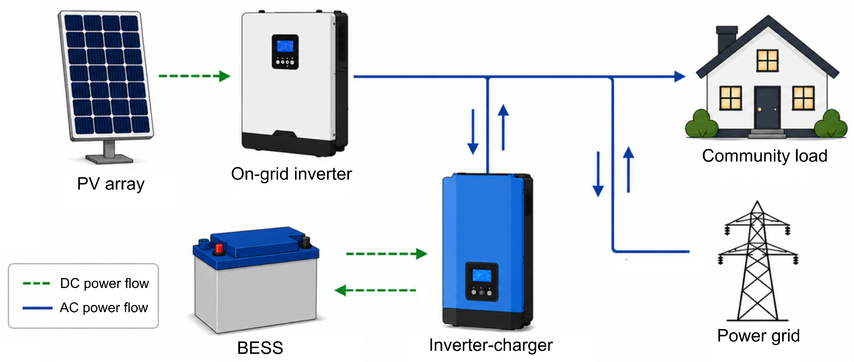
Figure 1 illustrates the first alternative, which combines an on-grid PV inverter with an inverter-charger and a battery bank. In this arrangement, the PV system primarily supplies the community demand and exchanges power with the utility grid through the on-grid inverter, whereas the inverter-charger manages the charging and discharging processes of the BESS. During grid outages, the inverter-charger enables islanded operation by supplying the community loads from the battery system, thereby allowing the microgrid to satisfy the imposed self-sufficiency requirements.

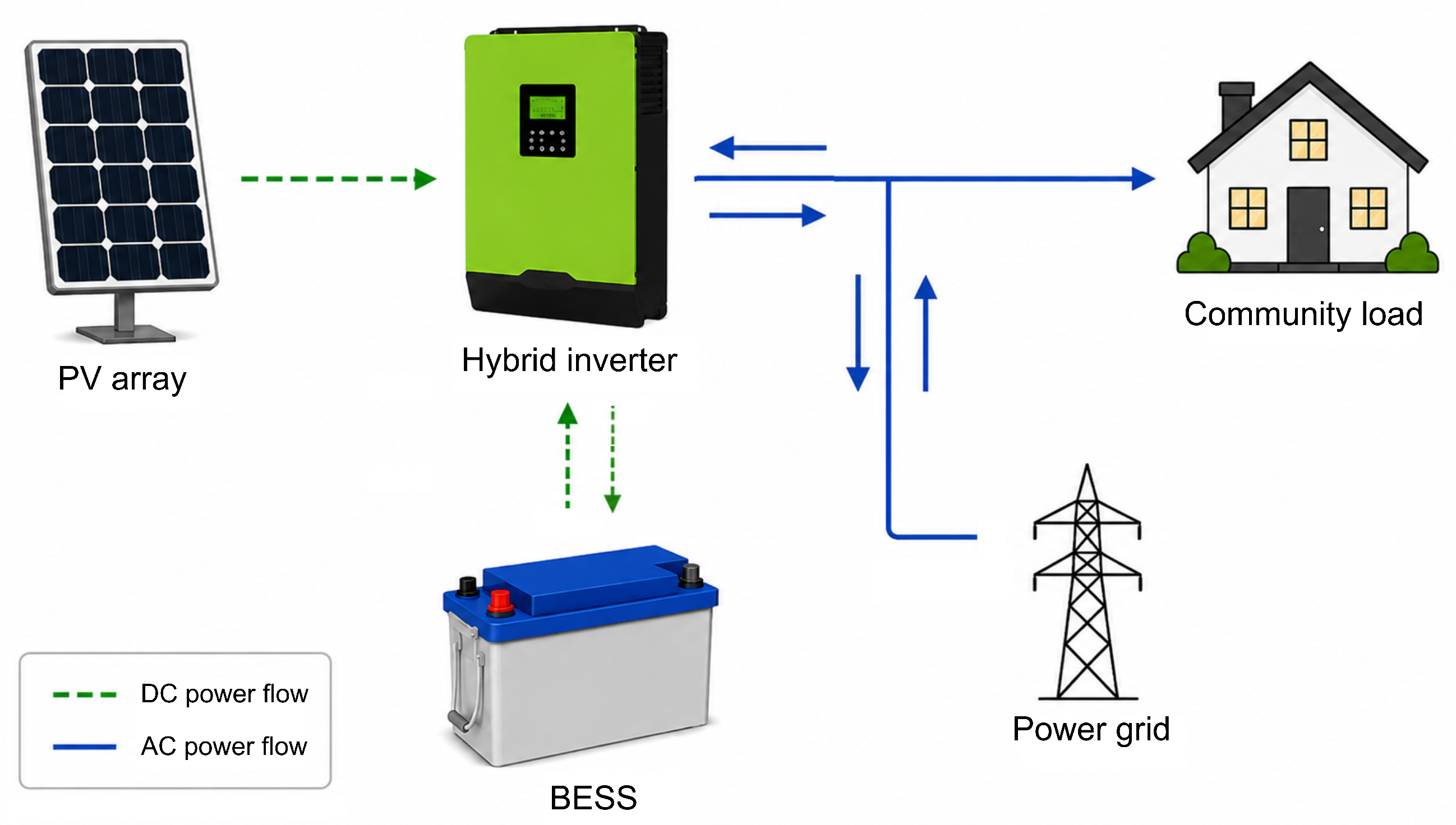
Figure 2 presents the second alternative, consisting of a PV system integrated with a hybrid inverter and a battery bank. In this configuration, the hybrid inverter directly manages the power flow among the PV array, the BESS, the utility grid, and the community loads, enabling both grid-connected and islanded operation. The battery system can be charged either by the PV generation or by importing energy from the utility grid, thereby increasing the operational flexibility of the microgrid while maintaining the required level of self-sufficiency.

The incorporation of these alternative configurations enables the proposed optimization framework to identify not only the optimal capacities of the microgrid assets but also the most appropriate technological architecture for each planning scenario. Consequently, the resulting solutions reflect the trade-offs among investment costs, operational performance, demand flexibility, and the reliability requirements established for the community microgrids under study.

2.2.2. Mathematical Formulation

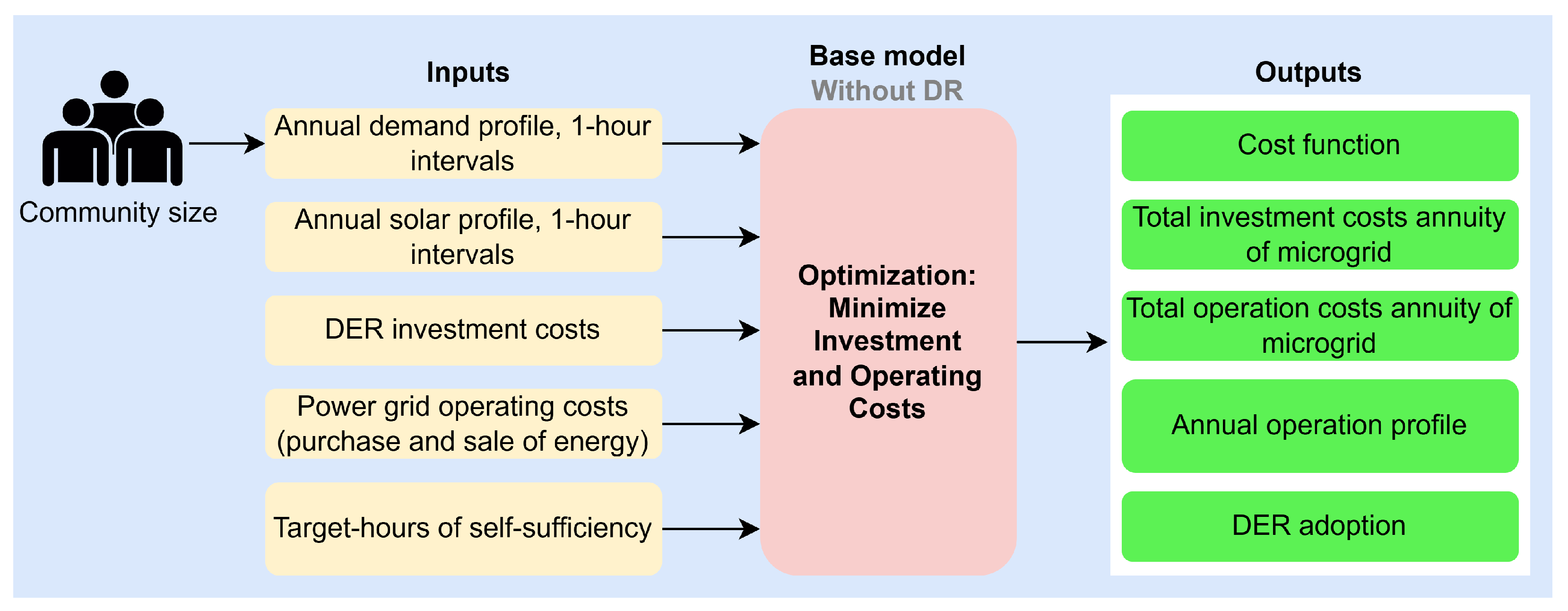
The Base Model aims to minimize investment and operational costs (energy purchases minus energy sales) for urban community microgrids that can operate autonomously during contingencies in the main power system. This is achieved through the optimal combination of PV and BESS. The model uses residential demand profiles, solar generation profiles, and economic parameters as inputs to determine the optimal adoption of distributed energy resources and the resulting operational costs. Figure 3 illustrates the overall structure of the Base Model.

The mathematical formulation of the model is presented below, beginning with the objective function defined in Equation (2).

$$\mathrm{I}.\mathrm{C}.=C_{\mathrm{PV}1}·P_{\mathrm{PV}1}+C_{\mathrm{PV}2}·P_{\mathrm{PV}2}+C_{\mathrm{BAT}}·E_{\mathrm{BAT}}+C_{\mathrm{ICh}}·P_{\mathrm{ICh}},$$

(1)

$$min\mathrm{I}.\mathrm{C}.+\sum _{t\in T}\left(C_{\mathrm{IMP}}·P_{\mathrm{IMP}}\left(t\right)-C_{\mathrm{EXP}}·P_{\mathrm{EXP}}\left(t\right)\right)·\mathsf{\Delta }t,$$

(2)

where $C_{\mathrm{PV}1}$, $C_{\mathrm{PV}2}$, $C_{\mathrm{BAT}}$ and $C_{\mathrm{ICh}}$ are the annual investment costs of the PV system with on-grid inverter technology, hybrid inverter, batteries and inverter charger, respectively. $C_{\mathrm{IMP}}$ and $C_{\mathrm{EXP}}$ are the prices for purchasing and selling electricity to the utility grid. $P_{\mathrm{IMP}}$ and $P_{\mathrm{EXP}}$ are the import and export powers to the power grid.

It should be noted that the BESS investment cost represents only the storage-capacity component (USD/kWh). Costs associated with power conversion equipment are accounted for separately through the inverter technologies included in the formulation. Specifically, the PV system cost incorporates the corresponding inverter technology (on-grid or hybrid). When an on-grid inverter is selected in combination with a BESS, an additional battery inverter-charger and its associated cost are explicitly considered and optimally sized.

Furthermore, the objective function is subject to a set of constraints related to the installed PV capacity, the selected inverter technology (on-grid or hybrid), BESS capacity, self-sufficiency requirements (reliability), the operational characteristics of the energy resources, and the mechanisms used to supply demand under both grid-connected and islanded operating conditions. The first set of constraints involves the PV capacity and its operation during the year considered. Constraints in (3) and (4) determine the type of PV system to install ($P_{\mathrm{PV}1}$ for on-grid inverter, and $P_{\mathrm{PV}2}$ for hybrid inverter). This decision is made using binary decision variables, $x_{\mathrm{PV}1}$ and $x_{\mathrm{PV}2}$, which along with (5), guarantee that only one of the two types is selected.

$$P_{\mathrm{PV}1}\le M·x_{\mathrm{PV}1},$$

(3)

$$P_{\mathrm{PV}2}\le M·x_{\mathrm{PV}2},$$

(4)

$$x_{\mathrm{PV}1}+x_{\mathrm{PV}2}\le 1.$$

(5)

The parameter M represents a sufficiently large positive constant used to enforce the relationship between binary and continuous decision variables. In this work, a value of $M=1000$ was adopted for all Big-M constraints.

Then, Equation (6) represents both PV technological alternatives considered in this work and determines the PV generation, $P_{\mathrm{PV}}\left(t\right)$, using the parameter $P{V}_{1\mathrm{kW}}\left(t\right)$, which represents the hourly generation profile of a 1 kW solar PV installation in the study region. Additionally, the power that can be injected into the grid, $P_{\mathrm{EXP}}\left(t\right)$, is limited by the available PV generation, as presented in Equation (7). Since constraints (3)–(5) ensure that only one PV technology can be selected, either $P_{PV1}$ or $P_{PV2}$ is forced to zero in the optimal solution. Consequently, $P_{\mathrm{PV}}\left(t\right)$ is automatically determined by the installed capacity associated with the selected configuration, either the on-grid inverter or the hybrid inverter.

$$P_{\mathrm{PV}}\left(t\right)=(P_{\mathrm{PV}1}+P_{\mathrm{PV}2})·P{V}_{1\mathrm{kW}}\left(t\right),$$

(6)

$$P_{\mathrm{EXP}}\left(t\right)\le P_{\mathrm{PV}}\left(t\right).$$

(7)

Furthermore, to account for the technical limits of battery operation and to extend its lifespan by preventing overcharging and deep discharging, the battery energy $E\left(t\right)$ cannot exceed 90% of its storage capacity $E_{\mathrm{BAT}}$, nor drop below 20%, as seen in (8) and (9), respectively [29]. Equation (10) shows the state of charge constraint, where $P_{\mathrm{cBAT}}\left(t\right)$ and $P_{\mathrm{dBAT}}\left(t\right)$ are the charging and discharging powers, respectively. Then, the efficiency rates of charge (${\eta }_{\mathrm{cBAT}}$) and discharge (${\eta }_{\mathrm{dBAT}}$) are both considered to be 90%, a value that already considers the inverter’s efficiency [30]. The study horizon comprises $T=8760$ hourly periods, with a temporal resolution of $\mathsf{\Delta }t=1$ hour. Equation (10) is enforced for $t=1,\dots ,T-1$, while the initial state of charge of the battery ($t=0$), is assumed to be equal to $90\%$ of the installed battery capacity.

$$E\left(t\right)\ge 0.2·E_{\mathrm{BAT}},$$

(8)

$$E\left(t\right)\le 0.9·E_{\mathrm{BAT}},$$

(9)

$$E\left(t\right)=E(t-1)+P_{\mathrm{cBAT}}\left(t\right)·{\eta }_{\mathrm{cBAT}}·\mathsf{\Delta }t-{\displaystyle \frac{P_{\mathrm{dBAT}}\left(t\right)}{{\eta }_{\mathrm{dBAT}}}}·\mathsf{\Delta }t.$$

(10)

In the event of a main power grid contingency, the BESS must ensure supply during a specific self-sufficiency period (i.e., target hours). To achieve this, (11) is incorporated into the model to ensure that the energy stored always meets or exceeds the sum of the difference between the demand, $D\left(t\right)$, total or critical demand, and the energy supplied by the PV system. d is a parameter that represents the target number of self-sufficiency periods of the microgrid.

$$E\left(i\right)\ge {\displaystyle \sum _{t=i}^{i+d-1}}\left(D\left(t\right)-P_{\mathrm{PV}}\left(t\right)\right)·\mathsf{\Delta }t,\forall i=\{0,1,2,3,\dots ,T-d\}.$$

(11)

It should be noted that the proposed self-sufficiency constraint is evaluated for all possible outage starting times throughout the annual simulation horizon. Consequently, the battery energy storage system must maintain sufficient energy reserves to satisfy the specified self-sufficiency requirement for every possible outage initiation time throughout the year. Although this formulation results in a conservative planning strategy, it enables the assessment of the additional investments required to ensure different levels of backup capability and energy autonomy in community microgrids.

Regarding the limits of the BESS charging and discharging power, (12)–(14) apply a similar principle as the PV system decision, considering binary variables $x_{\mathrm{cBAT}}\left(t\right)$ and $x_{\mathrm{dBAT}}\left(t\right)$. Therefore, the battery is not charged and discharged at the same time. Finally, (15) and (16) limit the power of the battery based on the inverter charger’s capacity, if the model decides to install an on-grid PV system, $P_{\mathrm{ICh}}$, or the capacity of the PV system with hybrid inverter, $P_{\mathrm{PV}2}$.

$$P_{\mathrm{cBAT}}\left(t\right)\le M·x_{\mathrm{cBAT}}\left(t\right),$$

(12)

$$P_{\mathrm{dBAT}}\left(t\right)\le M·x_{\mathrm{dBAT}}\left(t\right),$$

(13)

$$x_{\mathrm{cBAT}}\left(t\right)+x_{\mathrm{dBAT}}\left(t\right)\le 1,$$

(14)

$$P_{\mathrm{cBAT}}\left(t\right)\le P_{\mathrm{ICh}}+P_{\mathrm{PV}2},$$

(15)

$$P_{\mathrm{dBAT}}\left(t\right)\le P_{\mathrm{ICh}}+P_{\mathrm{PV}2}.$$

(16)

The minimum power of the battery inverter charger is constrained to be at least half the installed power of the on-grid system [31], or the maximum value between the sum of the total demand or the critical demand, during the target hours of self-sufficiency, such as is shown in (17). These constraints are implemented to ensure the operational feasibility of microgrids.

$$P_{\mathrm{ICh}}\ge max\left\{D\left(t\right),\forall t=\{0,1,2,3,\dots ,T-1\}\right\}.$$

(17)

The load is supplied at all times by those resources that the optimization model chooses to implement, as seen in (18), including the main power system, $P_{\mathrm{grid}}\left(t\right)$.

$$P_{\mathrm{IMP}}\left(t\right)+P_{\mathrm{PV}}\left(t\right)-P_{\mathrm{cBAT}}\left(t\right)+P_{\mathrm{dBAT}}\left(t\right)-P_{\mathrm{EXP}}\left(t\right)=D\left(t\right).$$

(18)

It is important to observe that if there is more PV generation than energy needs in the microgrid (including charging the storage) and if the main power system is available, this excess generation can be exported to the utility grid, $P_{\mathrm{EXP}}\left(t\right)$.

2.3. Planning and Operation Models with DR

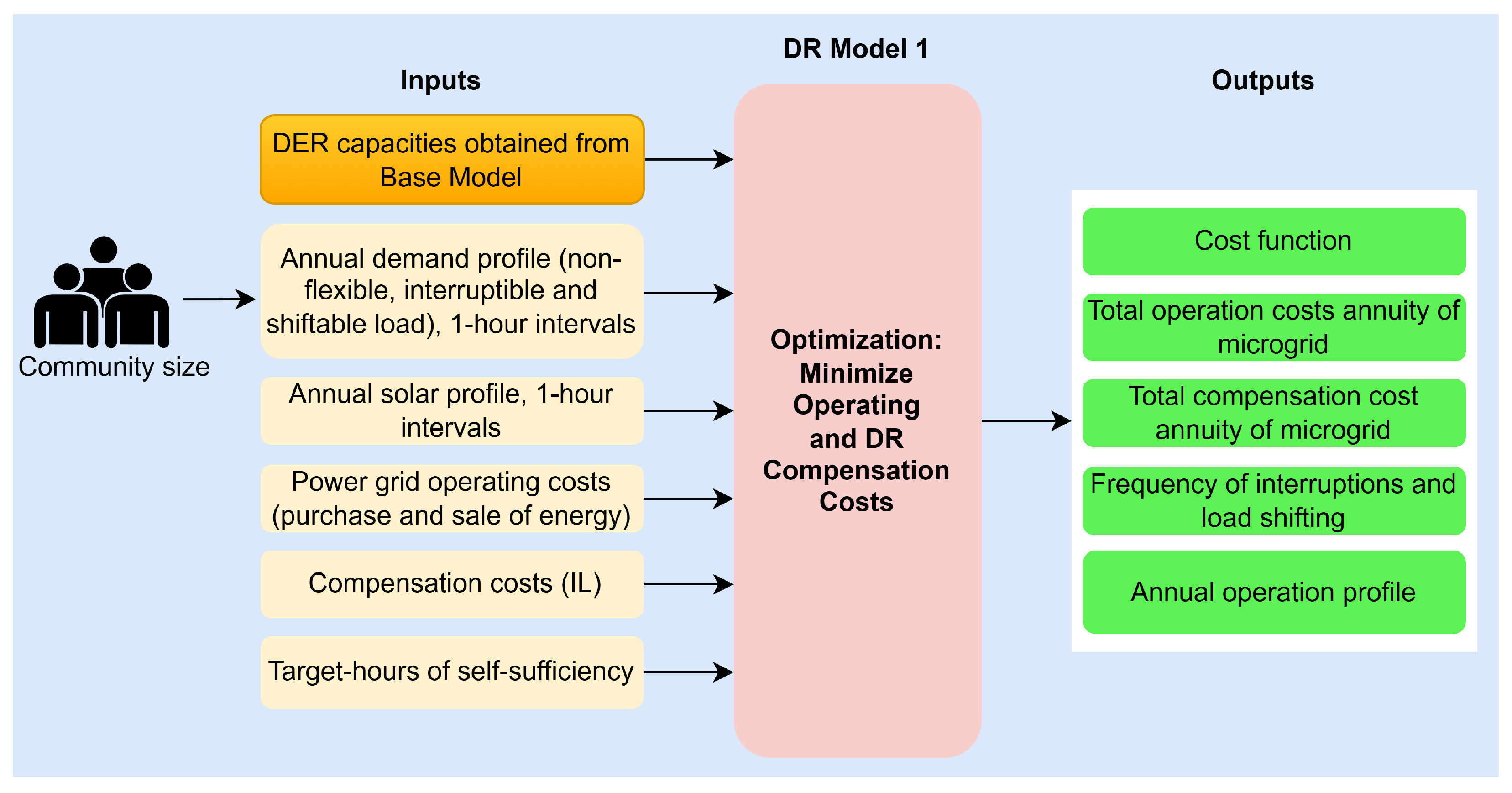
To integrate the active participation of end-users into the planning and operation of residential community microgrids, this study proposes two DR models. The first one, referred to as DRM1, is a microgrid operation model that incorporates DR while maintaining the DER capacities obtained from the Base Model. Specifically, DRM1 uses the investment decisions derived from the Base Model (without DR) to further reduce operational costs by utilizing flexible demand resources, including interruption and load shifting. Figure 4 presents the overall structure of DRM1. The objective function for this model is defined in (19). $C_{\mathrm{IL}}$ is the compensation cost, $D_{\mathrm{IL}}\left(t\right)$ is the interruptible load, and $IL\left(t\right)$ is a binary variable for interruptible load, which is defined in (23).

$$min\sum _{t\in T}\left(C_{\mathrm{IMP}}·P_{\mathrm{IMP}}\left(t\right)-C_{\mathrm{EXP}}·P_{\mathrm{EXP}}\left(t\right)\right)·\mathsf{\Delta }t+\sum _{t\in T}{C}_{\mathrm{IL}}·D_{\mathrm{IL}}\left(t\right)·IL\left(t\right)·\mathsf{\Delta }t.$$

(19)

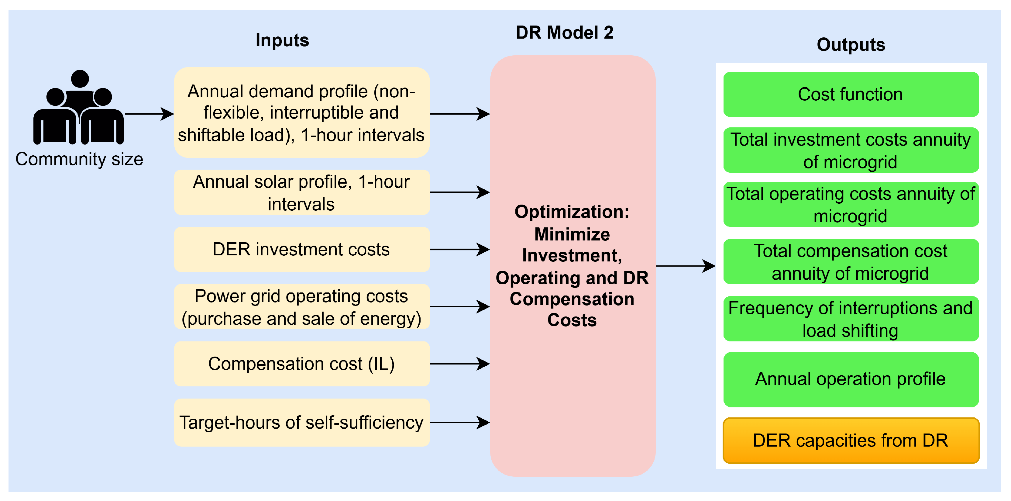
The second model, referred to as DRM2, aims to minimize investment, operational, and compensation costs while integrating the flexibility of demand resources directly within the optimization problem. This approach ensures that both investment and operational decisions consider the availability of DR. Figure 5 presents the overall structure of DRM2. The objective function for this model is defined in (20).

$$min\mathrm{I}.\mathrm{C}.+\sum _{t\in T}\left(C_{\mathrm{IMP}}·P_{\mathrm{IMP}}\left(t\right)-C_{\mathrm{EXP}}·P_{\mathrm{EXP}}\left(t\right)\right)·\mathsf{\Delta }t+\sum _{t\in T}{C}_{\mathrm{IL}}·D_{\mathrm{IL}}\left(t\right)·IL\left(t\right)·\mathsf{\Delta }t.$$

(20)

Regarding the power balance constraint, both DR models present the same structure according to (22), where a non-flexible load, $D_{\mathrm{NF}}\left(t\right)$, interruptible load, $D_{\mathrm{IL}}\left(t\right)$, and shiftable load $D_{\mathrm{SL}}\left(t\right)$, are optimally determined.

$$P_{\mathrm{IMP}}\left(t\right)+P_{\mathrm{PV}}\left(t\right)-P_{\mathrm{cBAT}}\left(t\right)+P_{\mathrm{dBAT}}\left(t\right)-P_{\mathrm{EXP}}\left(t\right)=D\left(t\right),$$

(21)

$$D_{\mathrm{NF}}\left(t\right)+D_{\mathrm{IL}}\left(t\right)·\left(1-IL\left(t\right)\right)+D_{\mathrm{SL}}\left(t\right)=D\left(t\right).$$

(22)

Both DR models are subject to the same constraints outlined in (3) to (17). Furthermore, to ensure demand flexibility, additional constraints have been integrated into the models. Here, the IL is represented by the household refrigerator. This selection is based on the fact that residential DR flexibility is commonly associated with thermal appliances and white goods, since thermal appliances can provide flexibility through their inherent thermal buffering capability [32]. In this context, the refrigerator can tolerate short-duration interruptions due to its thermal inertia, while preserving its primary function of food conservation. Therefore, a maximum interruption duration of 1 h is adopted in this work to avoid excessive loss of cold and to maintain food quality [33].

Duration of interruptions (23): the duration of an interruption must be shorter or equal to a maximum duration.

$${\displaystyle \sum _{h=t}^{t+d_{max}}}IL(h,u)\le d_{max}.$$

(23)

$IL(h,u)$ is a binary variable, assuming a value of 1 to indicate a load interruption. $d_{max}$ signifies the maximum interruption duration for user u, which in this work is set to 1 h, enough to maintain food quality without significant temperature rise [33].

Minimum interval between interruptions (24) and (25): To prevent the optimization model from continuously interrupting the load, a minimum time interval ($I_{min}$) between interruptions is set.

$${\displaystyle \sum _{h=t}^{t+d_{max}+I_{min}-1}}I{L}_{\mathrm{ST}}(h,u)\le 1,$$

(24)

$$I{L}_{\mathrm{ST}}(h,u)=\left\{\begin{array}{cc}IL(h,u),\hfill & h=0,\hfill \\ \left(IL(h,u)-IL(h-1,u)\right)·IL(h,u),\hfill & h\ge 1.\hfill \end{array}\right.$$

(25)

$I{L}_{\mathrm{ST}}(h,u)$ is a binary variable that assumes a value of 1 at the beginning of an interruption. Its calculation involves considering that for $h=0$ it is equivalent to the variable $IL(h,u)$, and for $h\ge 1$, it is the variation of the variable $IL(h,u)$ multiplied by itself. For this work, $I_{min}$ is set to 4 h. On the other hand, the SL is represented by the household washing machine. In (26) to (31), the constraints for the SL are proposed. It is important to clarify that these constraints assume that the management of the SL occurs within a single day.

Load Profile Size: Equation (26) guarantees that an SL profile p for a user u maintains size before and after an intra-daily shift.

$${\displaystyle \sum _{h=(n-1)·H}^{n·H-1}}pSL(p,h,u)=LPSize(p,u).$$

(26)

$pSL(p,h,u)$ is a three-dimensional binary variable (profile, period, and user), determining the activation status of profile p. It assumes a value of 1 during periods t when SL exceeds 0. Conversely, $pSL(p,h,u)$ is set to 0 when the SL equals 0. The size of each profile p is defined by the integer parameter $LPSize(p,u)$, which represents the number of periods during the shiftable load profile remains active. H denotes the number of periods in a day.

Continuity of load profile: The SL profile p must initiate only once within a period t of any day n. This requirement is determined by (27) and (28), where the three-dimensional binary variable $pS{L}_{\mathrm{ST}}(p,h,u)$ marks the beginning of each profile p at time t with a value of 1. This variable is calculated considering that for $h=0$ it is equivalent to the variable $pSL(p,h,u)$, and for $h\ge 1$ it is the variation of the variable $pSL(p,h,u)$ multiplied by itself.

$${\displaystyle \sum _{h=(n-1)·H}^{n·H-1}}pS{L}_{\mathrm{ST}}(p,h,u)=1,$$

(27)

$$pS{L}_{\mathrm{ST}}(p,h,u)=\left\{\begin{array}{cc}pSL(p,h,u),\hfill & h=0,\hfill \\ \left(pSL(p,h,u)-pSL(p,h-1,u)\right)·pSL(p,h,u),\hfill & h\ge 1.\hfill \end{array}\right.$$

(28)

No Load Profile Overlap: To prevent overlap between two or more SL profiles from the same user u within the same day, Equation (29) is introduced (e.g., the user can conduct multiple laundry cycles on the same day but not concurrently). This equation must be satisfied for each hour h, where $P_n$ represents the total number of shiftable load profiles available for user u:

$${\displaystyle \sum _{p=1}^{P_n}}pSL(p,h,u)\le 1.$$

(29)

Load Profile Conversion (30): This constraint aims to convert the binary representation of daily load profiles into real values, as depicted in (26) to (29).

$$pS{L}_{\mathrm{LOAD}}(p,h,u)={\displaystyle \sum _{k=0}^{min\{h,LPSize-1\}}}pS{L}_{\mathrm{ST}}(p,h-k,u)·profilesSL(p,k,u),$$

(30)

where $pS{L}_{\mathrm{LOAD}}(p,h,u)$ is a variable consisting of real values for all periods of a day n. $profilesSL(p,k,u)$ refers to each SL profile prior to optimization considering DR.

Integration of Daily Load Profiles: As the profiles obtained up to (30) represent daily patterns, each consisting of blocks or hourly periods, the addition of constraint (31), which must be satisfied for every hour h, guarantees the establishment of a load profile for each user u across the entire analysis period (one year):

$$D_{\mathrm{SL}}(n·H+h,u)={\displaystyle \sum _{p=1}^{P_n}}pS{L}_{\mathrm{LOAD}}(p,h,u),$$

(31)

where $D_{\mathrm{SL}}(n·H+h,u)$ denotes the resulting SL profile, indicating the adjusted shiftable load for user u over the entire analysis period.

3. Case Study

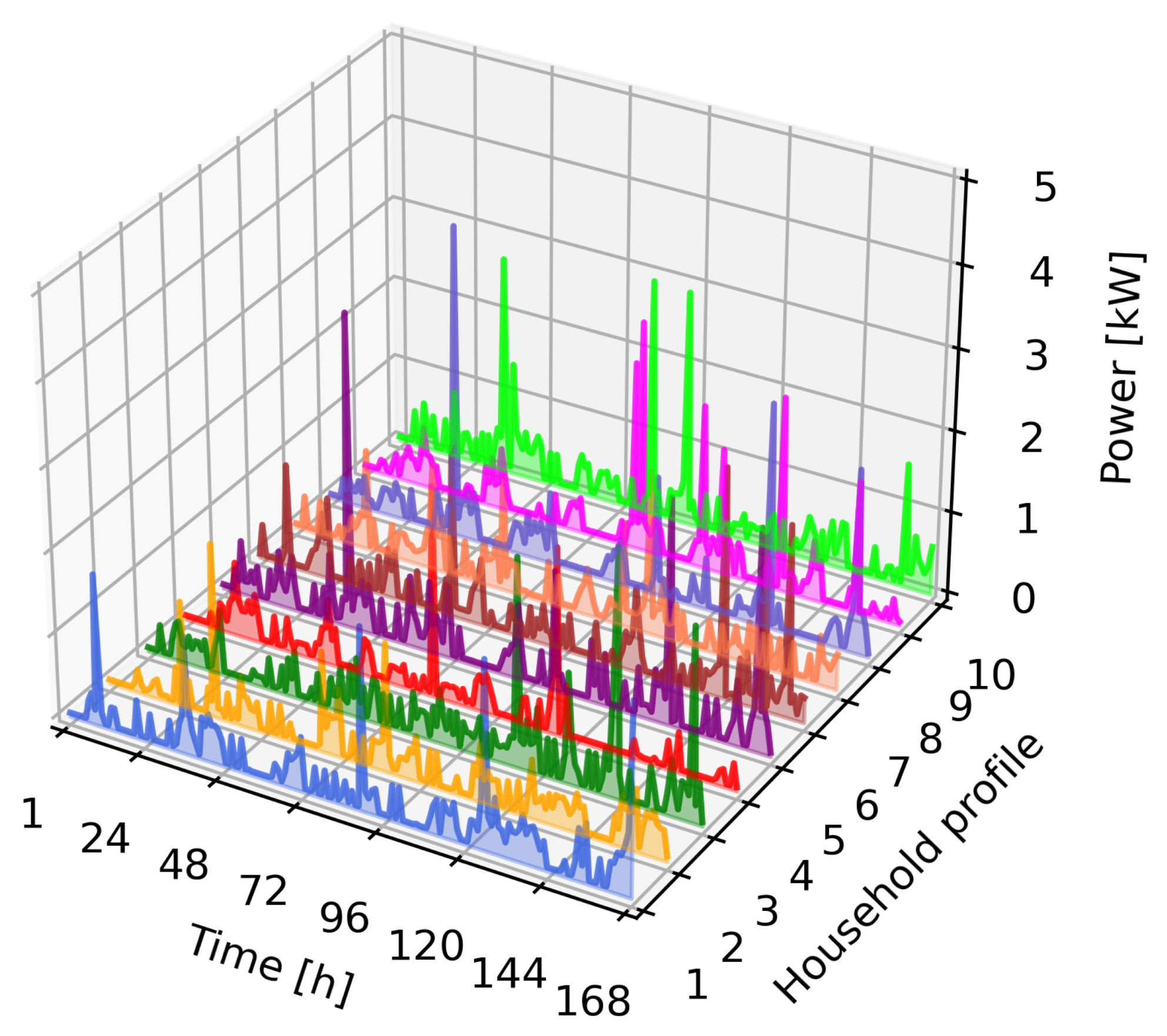
To evaluate the proposed community microgrid planning models, a database containing 4000 daily residential household load profiles was generated using the CREST Demand Model [27]. Load profiles were then randomly sampled from this database for each microgrid design. Figure 6 shows an example of 10 individual household profiles over a representative week of the analysis horizon. The variations among profiles highlight the importance of designing multiple microgrids for different community sizes rather than drawing conclusions from a single scenario. Therefore, microgrid designs were evaluated for communities comprising 1, 10, 20, 50, and 100 residential households.

The expected monthly energy consumption derived from the randomly generated demand profiles is 176 kWh, which reflects typical electricity consumption of residential customers in Colombia [34]. This value decreases to 90 kWh when only critical demand is considered. The load profiles also allow the expected energy consumption of flexible appliances to be determined. Specifically, the refrigerator and the washing machine have expected monthly consumptions of 31 kWh and 6.8 kWh, respectively, the latter corresponding to approximately 1 to 2 laundry cycles per week.

The annual solar profile was obtained from meteorological stations located in the study region of Valle del Cauca, Colombia, with observed capacity factors ranging from 11% to 20%. To adopt a conservative planning approach, the annual solar radiation profile corresponding to the lower bound of this capacity factor range was selected for the simulations. In addition, the investment annuity was calculated based on each asset’s cost, lifespan, and the applicable discount rate, which was set at 12%, as commonly used for public investment projects in Colombia [35].

Table 2. Economic parameters.

Parameter	Lifespan   [Years]	Value	Unit
On-grid PV system	20	92.6	USD/kW·year
Hybrid PV system	20	103.3	USD/kW·year
Inverter charger	10	69.9	USD/kW·year
Battery	15	40.3	USD/kWh·year
Energy purchase rate	–	0.204	USD/kWh
Energy sale rate	–	0.076	USD/kWh
Compensation rate (DR)	–	0.153	USD/kWh

summarizes the annualized investment costs for each feasible asset, as well as the rates associated with energy purchases, energy sales, and demand response compensation. All monetary values are expressed in United States Dollars (USD).

The energy sale price was set based on an analysis of the disaggregated tariff structures of selected Colombian electricity retailers. Since the generation component represented, on average, approximately 37% of the total retail electricity tariff, this value was adopted as the compensation rate for exported energy. Furthermore, due to the absence of a regulatory framework for residential demand response programs in Colombia, the compensation associated with interruptible demand was assumed to be equal to 75% of the prevailing electricity tariff. This compensation was exclusively applied to interruptible loads (i.e., refrigerators), whereas no explicit compensation was considered for shiftable loads. 100 oHptimal designs were generated for each community size and scenario. The analysis considered three target self-sufficiency durations (2 h, aligned with the Customer Average Interruption Duration Index (CAIDI) for urban areas in Colombia [36], as well as 4 and 6 h), two demand–supply scenarios (total demand and critical demand), and three planning models (Base Model, DRM1, and DRM2), resulting in approximately 7000 optimization problems. All optimization models were implemented in Python (version 3.13) and solved using the Gurobi Optimizer (version 12.0.0). The proposed formulations correspond to large-scale MILP problems with hourly resolution over an annual horizon (8760 periods). Simulations were performed on a workstation equipped with an Intel Core i7 processor (Lenovo, Medellín, Colombia) operating at 2.10 GHz, 16 GB of RAM, and Windows 10. Depending on the community size and planning model, solution times ranged from a few minutes for the Base Model to approximately 8 h for the largest DR cases considered in this study.

4. Results and Analysis

4.1. Baseline

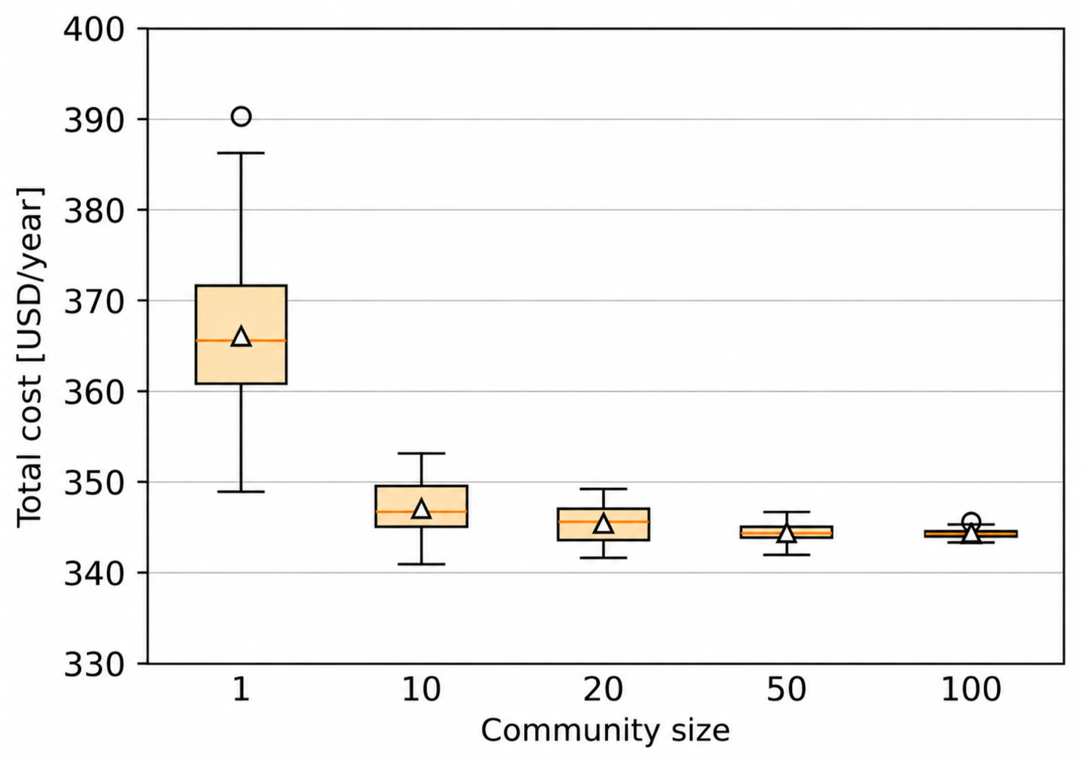
A baseline (BL) scenario is set without any reliability requirements, meaning zero target hours of self-sufficiency, which serves as a reference for comparing the total microgrid costs. By designing multiple community microgrids, different results are obtained for a given community size. Hence, to facilitate the comparison, the resulting optimal cost is divided by the number of households in the microgrid, being presented in this format throughout this work. This is illustrated in Figure 7, which shows a box plot of the objective function per household, containing 100 designs for each community size (BL scenario).

To complement the box-plot representation shown in Figure 7,

Table 3. Descriptive statistics of the annual total cost per household obtained from the 100 microgrid designs under the baseline scenario.

Community Size	Total Costs [USD/Year]—Baseline Scenario
	Mean	Median	Standard Deviation	Maximum	Minimum
1	366.0	365.4	7.9	390.4	348.7
10	346.9	346.5	3.1	353.0	340.8
20	345.3	345.6	2.3	349.1	341.6
50	344.2	344.2	1.1	346.6	341.9
100	344.2	344.1	0.7	345.5	343.1

reports descriptive statistics of the annual total cost per household obtained from the 100 microgrid designs developed for each community size under the baseline scenario. The reported indicators include the mean, median, standard deviation, maximum, and minimum values, providing additional insight into the effect of community size on both the expected costs and their variability.

The results indicate that increasing the community size reduces not only the expected annual cost per household but also the variability among the 100 optimal designs for each community. The mean annual cost decreases from 366.0 USD/year for a single household to approximately 344.2 USD/year in communities of 50 and 100 households, suggesting that most of the economic benefits of demand aggregation are achieved in medium-sized communities. Likewise, the standard deviation decreases from 7.9 to 0.7 USD/year, indicating more robust and predictable planning outcomes in larger communities. Finally, the close agreement between the mean and median values across all community sizes suggests relatively symmetric cost distributions with limited influence from extreme observations. These findings highlight the value of demand diversity in residential community microgrids, enabling both lower expected costs and reduced uncertainty in the planning process.

As the size increases, the standard deviation of all objective functions and the average cost among the 100 optimal designs decreases. For example, the average annual cost per household in communities of 20 households is around 12% lower than the highest cost for a single household (390.4 USD). This reduction is due to the presence of diversity among individual profiles within the microgrid. These savings underscore the important value of community in residential microgrid planning [28].

It is important to note that the BL scenario does not represent a grid-only configuration. Instead, it corresponds to the optimal microgrid design obtained with zero target hours of self-sufficiency. Under this condition, the optimization algorithm selected PV systems without BESS installations, since the absence of self-sufficiency requirements does not economically justify the adoption of energy storage systems. Therefore, the value of 390.4 USD/year corresponds to an optimally designed microgrid rather than to a household supplied exclusively by the conventional power grid.

4.2. The Additional Cost of Reliability

This section presents the outcomes of designing residential microgrids with different target hours of self-sufficiency, based on 100 designs for each community size. Thus,

Table 4. Expected maximum energy requirement per household as a function of target hours of self-sufficiency.

Target Hours of Self-Sufficiency [h]	Community Size [Households per Microgrid]	Total Demand [kWh]	Critical Demand [kWh]
2	1	5.4	1.4
	10	2.0	0.8
	20	1.8	0.7
	50	1.6	0.7
	100	1.5	0.6
4	1	7.6	2.3
	10	3.2	1.4
	20	2.8	1.2
	50	2.6	1.2
	100	2.5	1.1
6	1	9.3	2.9
	10	4.3	1.9
	20	3.9	1.7
	50	3.6	1.6
	100	3.5	1.6

shows the expected maximum energy requirement per household in each community throughout the analyzed year for total and critical demand. This result highlights an increase in energy demand if the target hours of self-sufficiency increase.

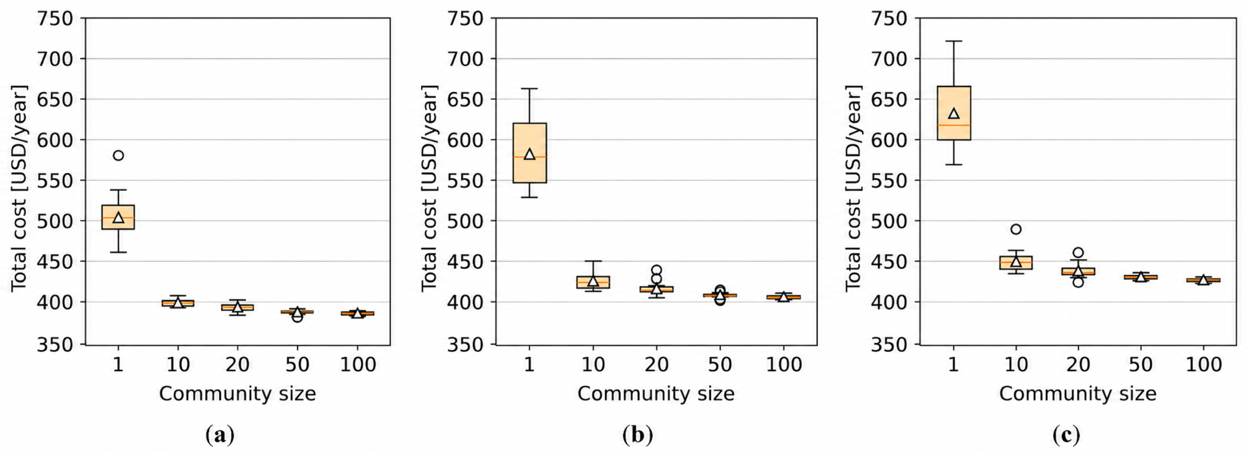
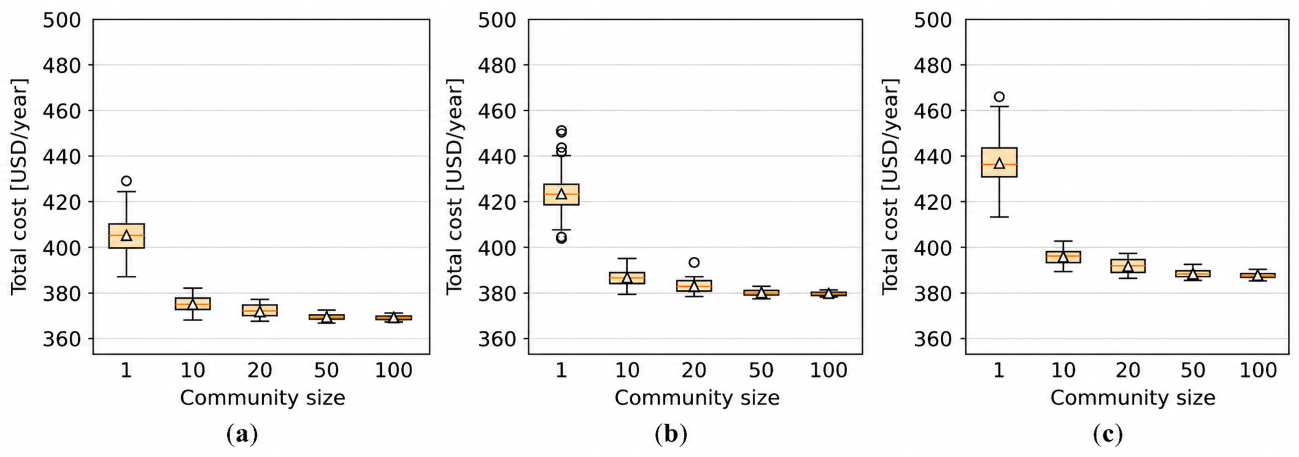
The total cost per household for each microgrid is presented in Figure 8 and Figure 9 for the total and critical demand cases, respectively. It is evident that as the target hours of self-sufficiency increase, the total cost of the microgrid for each community size rises compared to the BL. This increase is due to a greater capacity of PV system and BESS required to ensure total or critical demand supply at any time. The increase in investment costs associated with longer self-sufficiency durations reflects the conservative nature of the proposed formulation, which guarantees compliance with the self-sufficiency requirement regardless of when the outage occurs. Since the BESS must be capable of supporting outages occurring at any time during the year, larger storage capacities are required as the target self-sufficiency duration increases.

The importance of community associations is also emphasized. For instance, in communities of 20 households with 2 h back-up at any time with total demand supply (Figure 8a), these costs are 22.0% lower than those for single-household microgrids (505.1 USD).

Table 5. Increase in expected total cost per household as a function of target hours of self-sufficiency.

Community Size	Baseline [USD/Year]	Total Demand Supply			Critical Demand Supply
	0 h	2 h	4 h	6 h	2 h	4 h	6 h
1	366.0	38.0%	59.5%	73.0%	10.6%	15.6%	19.3%
10	346.9	15.0%	22.6%	30.0%	8.1%	11.3%	14.2%
20	345.3	14.1%	20.6%	27.4%	7.8%	10.9%	13.7%
50	344.2	12.9%	18.8%	25.5%	7.4%	10.4%	13.1%
100	344.2	12.4%	18.1%	24.5%	7.4%	10.2%	12.9%

details the percentage increase in expected total costs for each community compared to the BL. For example, in the case of 2 target hours of self-sufficiency, the expected total annual cost for a single-household community is 38.0% higher than the BL, and for community microgrids comprising 20 households, the expected total cost is only 14.1% higher. These values provide a direct estimate of the economic premium associated with guaranteeing reliability in residential community microgrids.

Although the additional costs associated with enhanced reliability can be quantified through the proposed methodology, their affordability may vary considerably across different socioeconomic contexts. Therefore, the acceptability of these cost increments should be assessed considering household income levels, access to financing mechanisms, prevailing electricity tariffs, and end-users’ willingness to pay for improved service continuity.

To provide further insight into the sources of the observed cost variations,

Table 6. Breakdown of the expected annual cost per household [USD/year] under the baseline scenario.

Cost Component	1	10	20	50	100
Total cost	366.0	346.9	345.3	344.2	344.2
PV Panels and Inverter	193.1	167.7	160.7	155.4	154.2
Battery bank	0.0	0.0	0.0	0.0	0.0
Inverter charger	0.0	0.0	0.0	0.0	0.0
Total investment	193.1	167.7	160.7	155.4	154.2
Energy purchase	289.0	262.5	261.7	260.6	260.7
Energy sales revenue	116.1	83.6	76.9	71.9	70.8

and

Table 7. Breakdown of the expected annual cost per household [USD/year] under the total demand supply scenario with 2 h of self-sufficiency.

Cost Component	1	10	20	50	100
Total cost	505.1	399.1	394.0	388.5	386.8
PV Panels and Inverter	252.2	172.1	164.2	156.8	153.6
Battery bank	230.7	88.4	79.7	71.1	67.1
Inverter charger	0.0	0.0	0.0	0.0	0.0
Total investment	483.0	260.5	244.0	227.9	220.6
Energy purchase	66.0	166.4	175.8	184.8	189.9
Energy sales revenue	43.9	27.8	25.7	24.3	23.7

present the expected annual cost per household and their main components for the BL scenario and for community microgrids with 2 h of self-sufficiency under the total demand supply scenario, respectively.

A comparison between Table 6 and Table 7 reveals that the increase in total costs associated with reliability requirements is primarily driven by the incorporation of battery energy storage systems and the expansion of PV capacity. For example, in communities of 20 households, the annual investment cost increases from 160.7 USD/year per household in the baseline scenario to 244.0 USD/year per household when 2 h of self-sufficiency are required. In contrast, the inverter charger cost remains zero in all scenarios because the optimization model did not select configurations requiring this component. Nevertheless, economies of scale remain evident, since larger communities exhibit lower investment costs per household due to demand diversity and resource sharing. These results indicate that improving reliability through community microgrid requires additional investments, primarily associated with the adoption of BESS and larger PV capacities. The economic attractiveness of these investments ultimately depends on household income levels, financing conditions, electricity tariff structures, and customers’ willingness to pay for enhanced reliability.

4.3. On the Value of Residential DR

In this section, potential savings derived from the flexibility of residential loads are explored (i.e., DR). Analyses were conducted across DRM1 and DRM2 models for the total demand scenario, and the corresponding expected total cost per household is presented in

Table 8. Expected DR savings per household for all microgrid planning models under the total demand supply scenario. Savings are calculated with respect to the corresponding Base Model cost.

Community	Target Hours of	Base Cost	DRM1	DRM2
Size	Self-Sufficiency	[USD/Year]	Savings [%]	Savings [%]
1	2 h	505.1	1.5	2.7
	4 h	583.9	0.9	2.8
	6 h	633.3	0.7	2.9
10	2 h	399.1	3.2	3.9
	4 h	425.2	2.8	4.2
	6 h	451.0	2.0	4.3
20	2 h	394.0	3.3	3.9
	4 h	416.3	3.1	4.4
	6 h	440.0	2.5	4.4

.

It is important to note that these costs are compared to the Base Model for each target hour of self-sufficiency. Savings from demand flexibility grow with the number of households per microgrid. In this context, the highest recorded DR savings are 4.4% per household within microgrid communities of 20 households. These findings indicate that, although residential demand response can reduce planning costs, its contribution remains modest compared with the additional investments required to guarantee reliability.

In DRM1, the savings from demand flexibility decrease as the target hours of self-sufficiency increase. This occurs because the DRM1 determines the adoption of DER (microgrid planning) for inflexible demand (without DR) with enough storage capacity to meet a larger portion of the demand. In contrast, DRM2 yields slightly greater benefits with increasing target hours of self-sufficiency. This occurs because the model leverages load interruption or shifting, thereby reducing unnecessary investment expenses for the community.

To analyze how the total costs of microgrids are influenced by the level of demand participation (DR),

Table 9. Expected DR savings per household for all microgrid planning models under the total demand supply scenario considering only load shifting. Savings are calculated with respect to the corresponding Base Model cost.

Community	Target Hours of	Base Cost	DRM1	DRM2
Size	Self-Sufficiency	[USD/Year]	Savings [%]	Savings [%]
1	2 h	505.1	0.6	1.3
	4 h	583.9	0.4	0.8
	6 h	633.3	0.3	0.8
10	2 h	399.1	0.9	0.9
	4 h	425.2	0.8	0.9
	6 h	451.0	0.6	1.1
20	2 h	394.0	0.9	0.9
	4 h	416.3	0.8	1.0
	6 h	440.0	0.8	1.1

presents the savings from DR when considering only load shifting. This analysis implies deactivating (23) and (24) in DR optimization models, named in this case, DRM1^′ and DRM2^′. These sensitivities confirm the previous conclusions, showing slightly higher benefits from DRM2 compared to DRM1. For instance, in the case of 6 h of self-sufficiency for communities of 20 households, the expected savings from DRM2^′ exceed those from DRM1^′ by just 0.3%. These results also highlight the role of interruptible loads in achieving cost savings per household.

A comparison of scenarios without interruptible loads (Table 9) and with participation of interruptible and shiftable loads (Table 8), reveals that shiftable loads contribute between 20% and 50% of DR savings, given a compensation cost for load interruption equivalent to 75% of the energy tariff price (Table 2). For example, in communities of 20 households with 2 h of self-sufficiency in the DRM2^′, savings from shiftable loads amount only to 0.9%. In contrast, when both interruptible and shiftable loads are active (DRM2 in Table 8), savings increase to 3.9%.

It should be noted that the demand response analysis was restricted to communities of 1, 10, and 20 households. Unlike the baseline microgrid planning model, the DRM1 and DRM2 models explicitly represent load interruption and load shifting decisions for each individual household over an annual horizon of 8760 time steps. Consequently, the number of continuous and binary decision variables increases substantially with community size, leading to significantly higher computational requirements.

It should be emphasized that the economic value of demand response depends on the assumptions regarding appliance flexibility, compensation mechanisms, and customer participation. Therefore, the savings reported in this study should be interpreted as representative of the considered residential scenarios rather than as universal limits for the value of demand response in community microgrids. Future work should investigate alternative demand response schemes and participation levels.

4.4. Der Adoption

To complement the findings outlined above,

Table 10. Expected PV adoption per household [kW] for all microgrid planning models under the total demand supply scenario.

Community Size	BL	Base Model			DRM1			DRM2
	0 h	2 h	4 h	6 h	2 h	4 h	6 h	2 h	4 h	6 h
1	2.09	2.44	2.58	2.61	2.44	2.58	2.61	2.34	2.48	2.52
10	1.81	1.67	2.02	2.31	1.67	2.02	2.31	1.60	1.92	2.17
20	1.73	1.59	1.90	2.22	1.59	1.90	2.22	1.53	1.80	2.10
50	1.68	1.52	1.80	2.13	–	–	–	–	–	–
100	1.67	1.49	1.77	2.08	–	–	–	–	–	–

illustrates the expected adoption of solar PV per household for each microgrid planning model. It is important to note that DRM1 uses the installed capacity obtained from the Base Model as an input parameter; therefore, the corresponding results are identical. This assumption reflects a scenario in which community energy assets have already been deployed and the community seeks to actively participate in DR programs to obtain additional benefits. Furthermore, the expected PV adoption per household generally decreases as the community size increases, reflecting the effects of demand diversity. As a result, DRM2 exhibits slightly lower PV adoption levels across all target hours of self-sufficiency and community sizes, since the combined use of load interruption and load shifting reduces the need for additional generation capacity.

On the other hand, the expected BESS adoption per household for all community sizes is presented in

Table 11. Expected BESS adoption per household [kW] for all microgrid planning models under the total demand supply scenario.

Community Size	BL	Base Model			DRM1			DRM2
	0 h	2 h	4 h	6 h	2 h	4 h	6 h	2 h	4 h	6 h
1	0.00	5.72	8.02	9.35	5.72	8.02	9.35	5.49	7.70	8.95
10	0.00	2.19	3.50	4.65	2.19	3.50	4.65	2.05	3.21	4.26
20	0.00	1.98	3.10	4.24	1.98	3.10	4.24	1.86	2.82	3.89
50	0.00	1.76	2.80	3.92	–	–	–	–	–	–
100	0.00	1.66	2.66	3.75	–	–	–	–	–	–

.

In larger communities, the expected BESS adoption decreases. However, it is evident that a higher number of target hours of self-sufficiency necessitates a larger storage system capacity. The deployment of the storage system is primarily guided by the self-sufficiency constraints (Equation (11)) to meet reliability requirements and minimize the operating costs of the microgrid, both in islanded mode and when connected to the power system. Without these constraints, the installation of BESS would not occur, as evidenced by the BL results. In addition, the DRM2 model installed slightly lower BESS capacities compared to the Base Model and DRM1 models, as it exploits both load interruption and load shifting capabilities. This approach contributes to reducing unnecessary investment costs for the community.

5. Conclusions

In this work, community microgrid planning models are developed to assess the additional cost of reliability required to provide households with different levels of self-sufficiency. Furthermore, the impact of incorporating demand response (DR) in the community microgrid planning process is explored to reveal its current value. To account for residential load variability, these models employ reliability constraints to optimize the adoption of photovoltaic (PV) panels and battery energy storage systems (BESS), ensuring that residential households can maintain autonomous energy supply at any time for a specified time window (i.e., target self-sufficiency durations of 0, 2, 4, and 6 h are considered).

After analyzing the results obtained from the different scenarios, the main conclusions are as follows:

1.

Guaranteeing predefined levels of self-sufficiency through reliability-constrained community microgrids requires additional investments whose magnitude depends on both the desired outage coverage duration and the community size. For instance, ensuring 2 h of self-sufficiency leads to an expected annual cost of 394 USD per household (a 14.1% increase compared to the Base Model for communities of 20 households), which may rise to 27.4% for 6 h. These results indicate that meaningful reliability improvements can be achieved with moderate increases in annual household costs.

2.

Under the assumptions adopted in this study, demand response provides only modest economic benefits in residential community microgrids. The developed models (DRM1 and DRM2) show maximum savings of 4.4% (around 20 USD per household annually), highlighting the still limited flexibility of residential demand, while also highlighting its potential relevance for future policy and regulatory developments.

3.

The value of community aggregation is confirmed in the development of urban community microgrids with reliability requirements. For example, in a 20-household community with 2 h of self-sufficiency, a cost reduction of 22% per household is achieved compared to individual systems. This is due to load diversity, which reduces aggregate peak demand and enables more efficient sizing of distributed energy resources.

Overall, the results suggest that community microgrids can effectively enhance reliability, although doing so requires additional investments whose magnitude depends on the desired level of self-sufficiency. Furthermore, the aggregation of households plays a key role in improving the economic performance of these systems, supporting their potential as a strategy to strengthen energy resilience in developing countries.

References

1. Levy, A.; Carrasco, J.J. Calidad y Confiabilidad de los Servicios eléCtricos en América Latina; Inter-American Development Bank: Washington, DC, USA, 2020. [Google Scholar]
2. Mina-Casaran, J.D.; Echeverry, D.F.; Lozano, C.A. Demand response integration in microgrid planning as a strategy for energy transition in power systems. IET Renew. Power Gener. 2021, 15, 889–902. [Google Scholar] [CrossRef] [Scilit]
3. Gilani, M.A.; Kazemi, A.; Ghasemi, M. Distribution system resilience enhancement by microgrid formation considering distributed energy resources. Energy 2020, 191, 116515. [Google Scholar] [CrossRef] [Scilit]
4. Gui, E.M.; MacGill, I.; Betz, R. Community microgrid investment planning: A conceptual framework. In Proceedings of the IEEE International Smart Cities Conference (ISC2), Kansas City, MO, USA, 16–19 September 2018; pp. 1–5. [Google Scholar]
5. Jimenez-Estevez, G.; Navarro-Espinosa, A.; Palma-Behnke, R.; Lanuzza, L.; Velazquez, N. Achieving resilience at distribution level: Learning from isolated community microgrids. IEEE Power Energy Mag. 2017, 15, 64–73. [Google Scholar] [CrossRef] [Scilit]
6. Hirsch, A.; Parag, Y.; Guerrero, J. Microgrids: A review of technologies, key drivers, and outstanding issues. Renew. Sustain. Energy Rev. 2018, 90, 402–411. [Google Scholar] [CrossRef] [Scilit]
7. Alcarruz, C.; Mina-Casaran, J.D.; Navarro-Espinosa, A. From passive network to PV urban community microgrids: Finding the optimal size and upgrading cost. Energy Sustain. Dev. 2022, 70, 387–402. [Google Scholar] [CrossRef] [Scilit]
8. You, S.; Zong, Y.; Bindner, H.W.; Lin, J.; Cai, Y.; Song, Y. Optimal dispatch of battery storage in an industrial microgrid with a mixed portfolio of renewables. In Proceedings of the International Conference on Power System Technology, Chengdu, China, 20–24 October 2014; pp. 3378–3383. [Google Scholar]
9. Rajab, Z.; Alfergani, A.; Asheibi, A.; Khalil, A.; Mohamed, F. Optimum microgrid planning and operation for improving reliability and power quality: Review. In Proceedings of the International Renewable Energy Congress (IREC), Hammamet, Tunisia, 23–25 October 2020; pp. 1–6. [Google Scholar]
10. Kumar, M.; Tyagi, B. Capital cost based planning and optimal sizing of a small community smart microgrid. In Proceedings of the International Conference on Knowledge and Smart Technology (KST), Pattaya, Thailand, 29 January–1 February 2020; pp. 121–126. [Google Scholar]
11. Zhou, J.; Weng, Z.; Li, J.; Song, X. Reliability evaluation, planning, and economic analysis of microgrid with access to renewable energy and electric vehicles. Electr. Power Syst. Res. 2024, 230, 110252. [Google Scholar] [CrossRef] [Scilit]
12. Dahiru, A.T.; Tan, C.W. Optimal sizing and techno-economic analysis of grid-connected nanogrid for tropical climates of the Savannah. Sustain. Cities Soc. 2020, 52, 101800. [Google Scholar]
13. Che, L.; Zhang, X.; Shahidehpour, M.; Alabdulwahab, A.; Abusorrah, A. Optimal interconnection planning of community microgrids with renewable energy sources. IEEE Trans. Smart Grid 2017, 8, 1054–1063. [Google Scholar]
14. Singh, M.K.; Kekatos, V.; Liu, C.-C. Optimal distribution system restoration with microgrids and distributed generators. In Proceedings of the IEEE Power & Energy Society General Meeting (PESGM), Atlanta, GA, USA, 4–8 August 2019; pp. 1–5. [Google Scholar]
15. Li, J.; Ma, X.-Y.; Liu, C.-C.; Schneider, K.P. Distribution system restoration with microgrids using spanning tree search. IEEE Trans. Power Syst. 2014, 29, 3021–3029. [Google Scholar] [CrossRef] [Scilit]
16. Xu, Y.; Liu, C.-C.; Schneider, K.P.; Tuffner, F.K.; Ton, D.T. Microgrids for service restoration to critical load in a resilient distribution system. IEEE Trans. Smart Grid 2018, 9, 426–437. [Google Scholar]
17. Boopathy, P.; Liyanage, M.; Deepa, N.; Velavali, M.; Reddy, S.; Maddikunta, P.K.R.; Khare, N.; Gadekallu, T.R.; Hwang, W.; Pham, Q.; et al. Deep learning for intelligent demand response and smart grids: A comprehensive survey. Comput. Sci. Rev. 2024, 51, 100591. [Google Scholar] [CrossRef] [Scilit]
18. Jordan, I.L.; O’Neill-Carrillo, E.; Lopez, N. Towards a zero net energy community microgrid. In Proceedings of the IEEE Conference on Technologies for Sustainability (SusTech), Phoenix, AZ, USA, 9–11 October 2016; pp. 63–67. [Google Scholar]
19. Zhu, L.; Zhou, X.; Zhang, X.P.; Yan, Z.; Guo, S.; Tang, L. Integrated resources planning in microgrids considering interruptible loads and shiftable loads. J. Mod. Power Syst. Clean Energy 2018, 6, 802–815. [Google Scholar] [CrossRef] [Scilit]
20. Majidi, M.; Nojavan, S. Optimal sizing of energy storage system in a renewable-based microgrid under flexible demand side management considering reliability and uncertainties. J. Oper. Autom. Power Eng. 2017, 5, 205–214. [Google Scholar] [CrossRef] [Scilit]
21. Kiptoo, M.K.; Lotfy, M.E.; Adewuyi, O.B.; Conteh, A.; Howlader, A.M.; Senjyu, T. Integrated approach for optimal techno-economic planning for high renewable energy-based isolated microgrid considering cost of energy storage and demand response strategies. Energy Convers. Manag. 2020, 215, 112904. [Google Scholar]
22. Qaeini, S.; Nazar, M.S.; Shafie-khah, M.; Osório, G.J.; Catalão, J.P.S. Optimal planning of CHP-based microgrids considering DERs and demand response programs. In Proceedings of the IEEE Mediterranean Electrotechnical Conference (MELECON), Palermo, Italy, 16–18 June 2020; pp. 605–610. [Google Scholar]
23. Haghifam, S.; Zare, K.; Dadashi, M. Bi-level operational planning of microgrids considering demand response technology and contingency analysis. IET Gener. Transm. Distrib. 2019, 13, 2721–2730. [Google Scholar]
24. Gazijahani, F.S.; Salehi, J. Reliability-constrained two-stage optimization of multiple renewable-based microgrids incorporating critical energy peak pricing demand response program using robust optimization approach. Energy 2018, 161, 999–1015. [Google Scholar]
25. Zhu, L.; Yan, Z.; Lee, W.J.; Yang, X.; Fu, Y.; Cao, W. Direct load control in microgrids to enhance the performance of integrated resources planning. IEEE Trans. Ind. Appl. 2015, 51, 3553–3560. [Google Scholar] [CrossRef] [Scilit]
26. Kiptoo, M.K.; Adewuyi, O.B.; Lotfy, M.E.; Amara, T.; Konneh, K.V.; Senjyu, T. Assessing the techno-economic benefits of flexible demand resources scheduling for renewable energy-based smart microgrid planning. Future Internet 2019, 11, 219. [Google Scholar]
27. McKenna, E.; Thomson, M. High-resolution stochastic integrated thermal-electrical domestic demand model. Appl. Energy 2016, 165, 445–461. [Google Scholar]
28. Mina-Casaran, J.D.; Echeverry, D.F.; Lozano, C.A.; Navarro-Espinosa, A. On the value of community association for microgrid development: Learnings from multiple deterministic and stochastic planning designs. Appl. Sci. 2021, 11, 6257. [Google Scholar] [CrossRef] [Scilit]
29. Truong, C.; Naumann, M.; Karl, R.C.; Müller, M.; Jossen, A.; Hesse, H.C. Economics of residential photovoltaic battery systems in Germany: The case of Tesla’s Powerwall. Batteries 2016, 2, 14. [Google Scholar] [CrossRef] [Scilit]
30. Šimić, Z.; Topić, D.; Knežević, G.; Pelin, D. Battery energy storage technologies overview. Int. J. Electr. Comput. Eng. Syst. 2021, 12, 53–65. [Google Scholar] [CrossRef] [Scilit]
31. Chen, X.; Du, Y.; Xiao, W.; Lu, S. Power ramp-rate control based on power forecasting for PV grid-tied systems with minimum energy storage. In Proceedings of the IEEE IECON, Beijing, China, 29 October–1 November 2017; pp. 2647–2652. [Google Scholar]
32. Klaassen, E.A.M.; Kobus, C.B.A.; Frunt, J.; Slootweg, J.G. Responsiveness of residential electricity demand to dynamic tariffs: Experiences from a large field test in the Netherlands. Appl. Energy 2016, 183, 1065–1074. [Google Scholar] [CrossRef] [Scilit]
33. Centers for Disease Control and Prevention. Keep Food Safe After a Disaster or Emergency. Available online: https://www.cdc.gov/food-safety/foods/keep-food-safe-after-emergency.html (accessed on 26 June 2024).
34. Consorcio Corpoema-CUSA. Caracterización Energética del Sector Residencial Urbano y Rural en Colombia; UPME (Unidad de Planeación Minero Energética): Bogotá, Colombia, 2012.
35. Departamento Nacional de Planeación. Justificación Técnica: Por la Cual se Adopta la Tasa Social de Descuento Como Parámetro en la Evaluación de Proyectos de Inversión del Sector Público; Departamento Nacional de Planeación: Bogotá, Colombia, 2022.
36. Superintendencia de Servicios Públicos Domiciliarios. Diagnóstico de la Calidad del Servicio de Energía eléCtrica en Colombia 2022; Superintendencia de Servicios Públicos Domiciliarios: Bogotá, Colombia, 2023.
Figure 1. Community microgrid configuration based on a grid-connected PV inverter, inverter-charger, and BESS.
Electricity 07 00067 g001
Figure 2. Community microgrid configuration based on a hybrid PV inverter and BESS.
Electricity 07 00067 g002
Figure 3. Structure of the proposed Base Model for community microgrid planning and operation.
Electricity 07 00067 g003
Figure 4. Structure of the proposed DR Model 1 (DRM1), where demand response is incorporated during the operational stage using the DER capacities obtained from the Base Model.
Electricity 07 00067 g004
Figure 5. Structure of the proposed DR Model 2 (DRM2), where demand response is integrated into the microgrid planning and operational optimization process.
Electricity 07 00067 g005
Figure 6. Example of randomly selected load demand profiles for communities.
Electricity 07 00067 g006
Figure 7. Box-plot of objective function per household of 100 microgrid designs.
Electricity 07 00067 g007
Figure 8. Box-plots of the objective function per household for 100 microgrid designs under total demand supply conditions: (a) 2 h, (b) 4 h, and (c) 6 h of self-sufficiency.
Electricity 07 00067 g008
Figure 9. Box-plots of the objective function per household for 100 microgrid designs under critical demand supply conditions: (a) 2 h, (b) 4 h, and (c) 6 h of self-sufficiency.
Electricity 07 00067 g009