Coordinated Robust Scheduling of Emergency Power Vehicles in Temporary Islanded Microgrids Considering Dynamic Frequency Constraints

Abstract

To address the transient frequency limit violations triggered by the low-inertia characteristics of temporary islanded microgrids formed under extreme disasters, this paper proposes a multi-source collaborative two-stage robust optimization day-ahead scheduling model considering dynamic frequency constraints. Firstly, a collaborative architecture encompassing emergency power vehicles, grid-forming energy storage systems, and flexible loads is constructed. Through collaborative scheduling in the day-ahead pre-scheduling and real-time re-scheduling stages, this architecture effectively avoids the exorbitant costs of physical load shedding under extreme conditions. Secondly, to overcome the limitations of traditional robust box uncertainty sets—which ignore temporal correlations, tend to cause non-physical high-frequency oscillations, and hinder algorithm convergence—a time-correlated uncertainty set based on state-transition auxiliary variables is designed to accurately capture the continuous evolution characteristics of meteorological disturbances. The column-and-constraint generation algorithm is utilized for the solution methodology, combined with the big-M method to transform the subproblem containing bilinear terms into a mixed-integer linear programming model for efficient solving. Simulation results on a modified 33-node test system demonstrate that the proposed model effectively filters out high-frequency oscillation trajectories and significantly improves computational efficiency. Under the worst-case temporal disturbances, the transient frequency drop and the rate of change in frequency are strictly controlled within safe thresholds. Compared to deterministic scheduling and traditional box-based robust models, the proposed scheme effectively balances system security and economic efficiency, demonstrating exceptional system resilience and defense capabilities against varying prediction errors.

1. Introduction

With the frequent occurrence of global extreme weather and natural disasters, enhancing the resilience of distribution networks has become a core issue in modern power system research [1]. Under emergency conditions where the main grid experiences power outages due to disasters, temporary islanded microgrids constructed using emergency power vehicles (EPVs), i.e., truck-mounted mobile diesel generator units, together with distributed renewable energy sources, can serve as an effective means to ensure continuous power supply for regional critical loads [2,3]. In an islanded operation, the microgrid no longer receives frequency support from the main grid. Meanwhile, the high penetration of inverter-interfaced renewable generation further reduces the equivalent inertia of the system. As a result, the temporary islanded microgrid exhibits typical low-inertia characteristics [4].

When facing sudden source-load changes caused by extreme disasters, low-inertia systems experience severe active power imbalances, which can trigger an excessive rate of change of frequency (RoCoF) and transient frequency nadir excursions, severely threatening the safety baseline and economic efficiency of the microgrid’s post-disaster emergency operation. Compared with large, interconnected power systems, temporary islanded microgrids are more vulnerable to frequency-security risks. Once disconnected from the main grid, the microgrid loses external frequency support, and its equivalent inertia is determined only by local synchronous and inverter-interfaced resources. Moreover, because the total capacity of an islanded microgrid is relatively small, the same MW-level source-load disturbance may correspond to a much larger per-unit power imbalance, resulting in a steeper RoCoF and a deeper transient frequency nadir. Therefore, RoCoF and frequency-nadir constraints are essential for ensuring secure operation in low-inertia islanded microgrids, especially when critical post-disaster loads must be continuously supplied [5,6]. From an operational perspective, these transient frequency–security issues also directly affect the economic performance of temporary islanded microgrids. Excessive RoCoF may trigger protection actions before slower reserves are fully activated, while a deep frequency nadir may require emergency physical load shedding to arrest the frequency decline. Since post-disaster islanded microgrids usually supply critical loads with limited local generation and reserve capacity, such emergency load shedding leads to high interruption penalties and reduces service restoration performance. Therefore, RoCoF and frequency-nadir constraints should be considered as key scheduling constraints rather than only as dynamic stability indices.

A grid-forming energy storage system (GFM-ESS) is widely regarded as an effective means of mitigating the inertia shortage in low-inertia islanded systems. References [7,8] conducted theoretical analyses on inertia support and frequency security in power system optimization problems, elucidating the necessity of considering frequency security constraints. Reference [9] incorporated dynamic frequency security constraints into an economic scheduling model; by introducing RoCoF and frequency nadir constraints, it proposed a frequency-secure optimal scheduling scheme considering synchronous inertia demands. At the control level, references [10,11] enhanced the grid-connection stability of grid-forming devices from the perspectives of adaptive virtual synchronous machine control and cascaded controller parameter tuning, respectively. At the scheduling level, reference [12] achieved the synchronous scheduling of multiple frequency response services within a stochastic unit commitment model. However, most of the aforementioned studies treat virtual inertia as a static parameter and rarely consider the coupling between the energy storage’s inertia support and its underlying state of charge (SoC) boundaries. In fact, the ability of GFM-ESS to release virtual inertia is constrained by its charging and discharging power as well as its remaining energy. If inertia control and energy boundary constraints are decoupled during scheduling, the system is highly prone to a collapse of the frequency defense line in extreme scenarios due to resource depletion [13,14]. Therefore, there is an urgent need to construct a multi-source collaborative scheduling framework that coordinates the physical inertia of EPVs, the virtual inertia of GFM-ESS, and flexible loads.

In terms of addressing source-load uncertainties, two-stage robust optimization has been widely applied in microgrid energy management [15]. However, many robust scheduling models use traditional box or polyhedral uncertainty sets. These sets usually treat disturbances in different time periods as mutually independent and therefore ignore the temporal correlation and continuity of meteorological evolution. As a result, the subproblem may generate non-physical extreme trajectories with abrupt jumps between adjacent periods. Such trajectories are unlikely to occur in real meteorological processes and may make the scheduling results overly conservative [16]. In addition, these unrealistic scenarios may reduce the efficiency of the column-and-constraint generation (C&CG) algorithm. The master problem has to add cuts generated from physically unlikely worst-case trajectories, which increases both the computational burden and the number of iterations. To address these issues, Reference [17] constructed a state-dependent wind power uncertainty set, validating the positive role of characterizing temporal features in improving operational economy. Reference [18] proposed a robust unit commitment model based on dynamic uncertainty sets. Reference [19] further established a robust optimization model that accounts for the temporal correlation of wind power prediction errors. Therefore, accurately capturing the continuous temporal evolution patterns of meteorological disturbances to reduce conservatism while ensuring computational feasibility has become a critical issue in enhancing the practicality of day-ahead scheduling schemes.

In summary, this paper proposes a coordinated two-stage robust day-ahead scheduling model for temporary islanded microgrids under post-disaster operating conditions. It should be emphasized that the column-and-constraint generation framework is adopted as a standard solution technique, rather than being claimed as a methodological novelty. The main contributions of this paper are summarized as follows.

(1) A multi-source coordinated frequency-secure scheduling framework is developed for temporary islanded microgrids supplied by emergency power vehicles, grid-forming energy storage systems, distributed photovoltaic units, and contracted flexible loads. Different from conventional robust microgrid scheduling models that mainly focus on steady-state power balance, the proposed model explicitly incorporates RoCoF and frequency-nadir constraints into the day-ahead robust scheduling process, thereby establishing a dynamic frequency defense baseline before real-time disturbances occur.

(2) A virtual-inertia-aware GFM-ESS scheduling model is embedded into the robust optimization framework. Instead of treating virtual inertia as a fixed parameter, the proposed formulation links the frequency-support capability of the GFM-ESS with its charging/discharging power, reserve allocation, and energy boundary constraints. Therefore, the optimizer can coordinate the mechanical inertia of EPVs, the virtual inertia of GFM-ESSs, and fast demand-side response while ensuring that the storage SoC constraints are not violated in both the day-ahead and real-time stages.

(3) A time-correlated uncertainty set based on state-transition auxiliary variables is constructed to characterize the continuous evolution of severe weather-induced PV and load disturbances. Unlike simply adjusting the conventional spatial uncertainty budget, the proposed temporal budget restricts the number of adjacent-period state transitions and therefore controls the continuity of uncertainty trajectories. This makes it possible to preserve persistent severe-weather patterns while excluding non-physical high-frequency switching scenarios generated by traditional box uncertainty sets.

(4) Case studies on a modified IEEE 33-node islanded microgrid demonstrate that the proposed model can reduce emergency physical load shedding, maintain RoCoF and frequency nadir within safety limits, and improve the computational performance of the C&CG process by filtering out physically unlikely worst-case trajectories.

2. System Modeling

The islanded microgrid system investigated in this study primarily comprises EPVs, GFM-ESS, distributed photovoltaic (PV) units, and flexible loads. In the conventional grid-connected mode, the frequency and voltage of the microgrid are supported by the main grid; however, in the islanded mode, the system lacks such support and exhibits typical low-inertia characteristics. The system must not only address the steady-state energy balance issues caused by source-load fluctuations but also guard against transient frequency instability risks triggered by sudden power imbalances. The proposed model is formulated from the perspective of a microgrid operator responsible for post-disaster islanded operation. During the temporary islanded period, the operator is assumed to have dispatch authority over the deployed EPVs, GFM-ESS units, PV curtailment, and contracted flexible loads, including shiftable loads and interruptible loads. Ordinary non-contracted loads are treated as fixed demand, while critical loads are prioritized and are not voluntarily curtailed. Forced physical load shedding is only used as an emergency recourse action when the available dispatchable and contracted resources are insufficient to maintain power balance and frequency security. The operator does not directly control all end-user loads. Only contracted flexible loads participate in demand response according to pre-signed agreements.

2.1. EPV Model

In this study, an EPV refers to a truck-mounted emergency diesel generator unit with a grid-connection interface, which is deployed as a mobile dispatchable power source for post-disaster service restoration. As the primary support power source for the islanded microgrid, the operation of an EPV is restricted by its mechanical rotor inertia and governor response characteristics. Its operation must satisfy startup and shutdown logic, steady-state ramping, and transient reserve constraints. The operational status and start-stop logic of the units are expressed as

$$u_{i,t}-u_{i,t-1}=y_{on,i,t}-y_{off,i,t}, \forall i,\forall t$$

(1)

$$y_{on,i,t}+y_{off,i,t}\le 1, \forall i,\forall t$$

(2)

where $u_{i,t}$ denotes the operational state of EPV during period t, while $y_{on,i,t}$ and $y_{off,i,t}$ represent the startup and shutdown variables, respectively.

To ensure the safe operation of the units, the active power output must be restricted within the allowable physical range, and minimum startup and shutdown time requirements must be satisfied:

$$P_{EPV,i}^{min}{u}_{i,t}\le P_{EPV,i,t}\le P_{EPV,i}^{max}{u}_{i,t}, \forall i,\forall t$$

(3)

$${\displaystyle \sum _{\tau =t}^{t+T_{on}^i-1}}{u}_{i,\tau }\ge T_{on}^i{y}_{on,i,t}, \forall i,t=1,\dots ,T-T_{on}^i+1$$

(4)

$${\displaystyle \sum _{\tau =t}^{t+T_{off}^i-1}}\left(1-u_{i,\tau }\right)\ge T_{off}^i{y}_{off,i,t}, \forall i,t=1,\dots ,T-T_{off}^i+1$$

(5)

where $P_{EPV,i,t}$ is the active power output of the EPV; $P_{EPV,i}^{min}$ and $P_{EPV,i}^{max}$ are the lower and upper output limits; and $T_{on}^i$ and $T_{off}^i$ are the minimum startup and shutdown time parameters.

The adjustment of unit output in adjacent periods is restricted by the steady-state ramp rate, and primary frequency regulation reserves must be pre-allocated to cope with transient frequency drops:

$$-R_{EPV,i}^{down}\le P_{EPV,i,t}-P_{EPV,i,t-1}\le R_{EPV,i}^{up}, \forall i,\forall t$$

(6)

$$0\le R_{EPV,i,t}^{freq}\le R_{EPV,i}^{freq,max}, \forall i,\forall t$$

(7)

$$P_{EPV,i,t}+R_{EPV,i,t}^{freq}\le P_{EPV,i}^{max}{u}_{i,t}, \forall i,\forall t$$

(8)

where $R_{EPV,i}^{up}$ and $R_{EPV,i}^{down}$ are the upper limits of the steady-state ramp rate; $R_{EPV,i,t}^{freq}$ represents the primary frequency regulation reserve capacity, the upper limit of which is constrained by the maximum transient physical ramping capability of the unit, denoted as $R_{EPV,i}^{freq,max}$.

2.2. GFM-ESS Model

Unlike traditional grid-following storage, the GFM-ESS establishes and maintains the grid voltage and frequency through inverter control strategies. Its charging/discharging power and SoC must satisfy temporal energy continuity constraints:

$$0\le P_{dis,e,t}\le P_{ESS,e}^{max}(1-v_{e,t}), \forall \mathrm{e},\forall t$$

(9)

$$0\le P_{ch,e,t}\le P_{ESS,e}^{max}{v}_{e,t}, \forall \mathrm{e},\forall t$$

(10)

$$E_{e,t}=E_{e,t-1}+({\eta }_{ch}{P}_{ch,e,t}-{\displaystyle \frac{P_{dis,e,t}}{{\eta }_{dis}}}), \forall \mathrm{e},\forall t$$

(11)

$$E_e^{min}\le E_{e,t}\le E_e^{max}, \forall \mathrm{e},\forall t$$

(12)

$$E_{e,T}=E_{e,0}, \forall \mathrm{e},\forall t$$

(13)

where $v_{e,t}$ is a mutual exclusivity variable to prevent simultaneous charging and discharging; $P_{dis,e,t}$ and $P_{ch,e,t}$ are the discharging and charging powers; $P_{ESS,e}^{max}$ is the rated power of the inverter; $E_{e,t}$ is the stored energy; ${\eta }_{dis}$ and ${\eta }_{ch}$ are the discharging and charging efficiencies; $E_e^{max}$ and $E_e^{min}$ are the allowable safety limits for the stored energy; and $E_{e,0}$ and $E_{e,T}$ represent the initial and final energy states within the scheduling cycle, ensuring intra-day energy conservation and availability for the following day.

It should be noted that the storage energy boundary in Equation (12) is enforced as a hard physical constraint in both the day-ahead pre-scheduling stage and the real-time re-scheduling stage. Real-time source-load fluctuations are not assumed to be absorbed solely by the GFM-ESS. Instead, they are jointly handled by GFM-ESS charging/discharging adjustment, pre-allocated frequency reserves, EPV primary frequency response, PV curtailment, contracted flexible loads, and emergency load shedding when necessary. Therefore, the GFM-ESS can only provide regulation and virtual inertia within its feasible power and energy ranges. If the available storage energy is insufficient, the model activates other recourse actions rather than relaxing or violating the SoC constraint.

When providing frequency support, the reserves pre-allocated by the storage are restricted not only by the power upper limit but also by the remaining energy [20]:

$$P_{dis,e,t}+R_{up,e,t}^{freq}\le k_g{P}_{ESS,e}^{max}, \forall \mathrm{e},\forall t$$

(14)

$$P_{ch,e,t}+R_{down,e,t}^{freq}\le k_g{P}_{ESS,e}^{max}, \forall \mathrm{e},\forall t$$

(15)

$$E_{e,t}-{\displaystyle \frac{R_{up,e,t}^{freq}}{{\eta }_{dis}}}{T}_{sus}\ge E_e^{min}, \forall \mathrm{e},\forall t$$

(16)

$$E_{e,t}+{\eta }_{ch}{R}_{down,e,t}^{freq}{T}_{sus}\le E_e^{max}, \forall \mathrm{e},\forall t$$

(17)

where $R_{up,e,t}^{freq}$ and $R_{down,e,t}^{freq}$ are the upward and downward frequency regulation reserves; $k_g$ is the short-term overload coefficient of the inverter; and $T_{sus}$ is the required sustained time.

The inertia support capability of the GFM-ESS stems from its power response capability [21]. Let $H_{vir,e,t}$ be the equivalent inertia constant, which is proportional to the transmission power of the interface line. When the energy released by the storage is large, the inertia constant is large, and the RoCoF is relatively small, which is conducive to maintaining system power balance. Conversely, when the energy released is small, the inertia constant is small, and the RoCoF is larger, potentially causing frequency stability issues.

$$H_{vir,e,t}=H_e^{min}+(H_e^{max}-H_e^{min}){\displaystyle \frac{P_{dis,e,t}+P_{ch,e,t}}{P_{ESS,e}^{max}}}$$

(18)

where $H_e^{max}$ and $H_e^{min}$ are the upper and lower virtual inertia limits.

It should be noted that Equation (18) assumes that the GFM-ESS remains electrically connected and operates in grid-forming mode during the islanded scheduling horizon. Therefore, even when $P_{dis,e,t}=0$ and $P_{ch,e,t}=0$, the GFM-ESS can still provide the floor-level virtual inertia $H_e^{min}$ through its baseline voltage- and frequency-forming control. This standby grid-forming mode has a scheduling implication: the optimizer may keep a storage unit online to contribute minimum inertia support even when it does not exchange steady-state active power with the microgrid.

2.3. Flexible Load and PV Model

Flexible resources within the islanded microgrid primarily consist of demand-side shiftable loads (SLs) and interruptible loads (ILs). Rational deployment of these resources is crucial for maintaining power balance and coping with transient impacts.

SLs participate in scheduling by transferring power demand across periods. The shifted-in and shifted-out powers are restricted by the maximum participation ratio stipulated in user agreements and must satisfy total energy conservation throughout the scheduling cycle:

$$0\le P_{SL,t}^{in}\le {\alpha }_{SL}{P}_{load,t}^{fore}$$

(19)

$$0\le P_{SL,t}^{out}\le {\alpha }_{SL}{P}_{load,t}^{fore}$$

(20)

$${\displaystyle \sum _{t=1}^T}{P}_{SL,t}^{in}={\displaystyle \sum _{t=1}^T}{P}_{SL,t}^{out}$$

(21)

where $P_{SL,t}^{in}$ and $P_{SL,t}^{out}$ are the shifted-in and shifted-out powers; $P_{load,t}^{fore}$ is the forecasted baseline load; and ${\alpha }_{SL}$ is the maximum allowable proportion of the SL.

ILs can be directly curtailed during emergencies such as power deficits. To protect the basic production benefits of industrial users, load shedding cannot be unlimited [22]. The curtailed power must satisfy a single-period ratio upper limit, and the total energy called upon throughout the day must be constrained by the contract budget:

$$0\le P_{IL,t}\le {\beta }_{IL}{P}_{load,t}^{fore}$$

(22)

$${\displaystyle \sum _{t=1}^T}{P}_{IL,t}\Delta t\le E_{IL}^{budget}$$

(23)

where $P_{IL,t}$ is the actual curtailed power; ${\beta }_{IL}$ is the maximum curtailment ratio; and $E_{IL}^{budget}$ is the total energy budget limit.

For distributed PV, curtailment is permitted during extreme downward regulation or when the storage capacity reaches its limit. The curtailed amount is restricted by the current available generation capacity:

$$0\le P_{curt,t}\le P_{PV,t}^{act}$$

(24)

where $P_{curt,t}$ is the actual PV curtailment power and $P_{PV,t}^{act}$ is the actual available output of the distributed PV at period t.

2.4. Network Power Flow Constraints

A linearized branch flow model (DistFlow) is employed to characterize the physical operational boundaries of the microgrid:

$$P_{j,t}^{inj}=\sum _{k\in \delta \left(j\right)}{P}_{jk,t}-\sum _{i\in \pi \left(j\right)}{P}_{ij,t}$$

(25)

$$Q_{j,t}^{inj}=\sum _{k\in \delta \left(j\right)}{Q}_{jk,t}-\sum _{i\in \pi \left(j\right)}{Q}_{ij,t}$$

(26)

$$U_{j,t}=U_{i,t}-2(R_{ij}{P}_{ij,t}+X_{ij}{Q}_{ij,t})$$

(27)

$${\left(U^{min}\right)}^2\le U_{j,t}\le {\left(U^{max}\right)}^2$$

(28)

where $P_{j,t}^{inj}$ and $Q_{j,t}^{inj}$ are the active and reactive power injected at node j; $P_{ij,t}$ and $Q_{ij,t}$ are the branch active and reactive power flows; $U_{j,t}$ is the square of the node voltage magnitude; $R_{ij}$ and $X_{ij}$ are the branch resistance and reactance parameters; $U^{min}$ and $U^{max}$ are the safety limits for the node voltage magnitude; and $\delta \left(j\right)$ and $\pi \left(j\right)$ denote the sets of branches with node j as the sending and receiving ends, respectively.

Regarding line capacity, the true physical feasible region is a non-linear quadratic circular domain. To overcome the pseudo-feasible region generated by traditional box relaxation and ensure the linearity of the two-stage RO subproblem, a regular octahedral polyhedral approximation is adopted for high-precision linear approximation:

$$-S_{max}^{ij}\le P_{ij,t}\le S_{max}^{ij}$$

(29)

$$-S_{max}^{ij}\le Q_{ij,t}\le S_{max}^{ij}$$

(30)

$$-\sqrt{2}{S}_{max}^{ij}\le P_{ij,t}+Q_{ij,t}\le {\sqrt{2}S}_{max}^{ij}$$

(31)

$$-\sqrt{2}{S}_{max}^{ij}\le P_{ij,t}-Q_{ij,t}\le {\sqrt{2}S}_{max}^{ij}$$

(32)

where $S_{max}^{ij}$ is the apparent power capacity limit. Equations (29)–(32) transform the non-linear capacity boundary into purely linear inequalities through multiple linear hyperplanes with different slopes, ensuring power flow security under source-load disturbances.

2.5. Dynamic Frequency Security Constraints with Virtual Inertia

In the event of a sudden active-power deficit, the islanded microgrid faces the risks of excessive RoCoF and frequency nadir violations because it lacks voltage and frequency support from the main grid. The total equivalent inertia $H_{sys,t}$ of the system at period t is contributed by the physical mechanical inertia of the online EPVs and the virtual inertia of the GFM-ESSs. Following the standard per-unit swing-equation formulation, the aggregated system inertia is normalized by the system power base:

$$H_{sys,t}={\displaystyle \frac{{\displaystyle {\sum }_{i=1}^{N_{EPV}}}{H}_{EPV,i}{S}_{EPV,i}{u}_{i,t}+{\displaystyle {\sum }_{e=1}^{N_{ESS}}}{H}_{vir,e,t}{S}_{INV,e}}{S_{base}}}$$

(33)

where $N_{EPV}$ and $N_{Ess}$ denote the total number of EPVs and GFM-ESS units, respectively; $H_{EPV,i}$ and $S_{EPV,i}$ represent the physical mechanical inertia constant and the rated capacity of EPV; $S_{INV,e}$ is the rated capacity of the inverter for GFM-ESS; and $S_{base}$ is the system base power. With this normalization,$H_{sys,t}$ is expressed in seconds and the active-power imbalance terms used in the frequency-security constraints are expressed per unit.

The equivalent center-of-inertia swing equation for the low-inertia microgrid is written as follows:

$${\displaystyle \frac{2H_{sys,t}}{f_0}}·{\displaystyle \frac{d\Delta f\left(t\right)}{dt}}=\Delta p(t)$$

(34)

where $\Delta f\left(t\right)$ is the system frequency deviation; $\Delta p\left(t\right)$ is the active power imbalance; $f_0$ is the initial frequency.

Let $\Delta P_{PV,t}$ denote the PV-output shortfall caused by the uncertainty realization and let $\Delta P_{load,t}$ denote the load-demand increase. The total active-power deficit caused by the source-load disturbance is defined as

$$P_{drop,t}^{total}=\Delta P_{PV,t}+\Delta P_{load,t},\forall t$$

(35)

The corresponding per-unit active-power deficit is

$$p_{drop,t}^{total}={\displaystyle \frac{P_{drop,t}^{total}}{S_{base}}}$$

(36)

Similarly, the emergency physical load shedding used in the frequency-security constraints is also expressed per unit:

$$p_{shed,t}={\displaystyle \frac{P_{shed,t}}{S_{base}}}$$

(37)

At the initial instant of the microgrid encountering a disturbance, no reserve resources are activated, and the system power deficit reaches its peak. To satisfy the maximum allowable RoCoF limit ${RoCoF}_{max}^{limit}$, the initial net disturbance power $\Delta p$ must be restricted by the current inertia boundary of the system. Since emergency physical load shedding acts as the last instantaneous defense measure to arrest the frequency drop, the net disturbance at this moment is $\Delta p=p_{drop,t}^{total}-p_{shed,t}$. Consequently, Equation (34) is transformed into the following linear inequality boundary:

$$p_{drop,t}^{total}-p_{shed,t}\le {\displaystyle \frac{2{RoCoF}_{max}^{limit}}{f_0}}{H}_{sys,t}$$

(38)

Substituting Equations (18) and (33) into Equation (38) yields an affine inequality in the decision variables $P_{dis,e,t}$, $P_{ch,e,t}$, $u_{i,t}$, and $p_{shed,t}$. This is because $H_{vir,e,t}$ is an affine function of the charging and discharging powers, while $S_{base}$, $S_{EPV,i}$, $S_{INV,e}$, $f_0$, and ${RoCoF}_{max}^{limit}$ are constants. Therefore, the RoCoF constraint remains linear and does not require any additional linearization.

The nadir constraint aims to ensure that the minimum frequency of the system after a disturbance is not lower than the safety limit ${\Delta f}_{max}$. Integrating Equation (34) in the time domain from the occurrence of the disturbance to the time of the frequency nadir yields

$${\int }_0^{\tau }\left({\Delta p}_{net}-{\Delta p}_{response}\left(t\right)\right)dt={\displaystyle \frac{2H_{sys,t}}{f_0}}{\Delta f}_{max}$$

(39)

where ${\Delta p}_{net}$ is the initial net active power deficit of the system; ${\Delta p}_{response}(t)$ is the sum of the dynamic active power support responses provided by various reserve resources during the transient process; and $\tau$ is the critical time window to reach the frequency nadir.

ILs possess fast frequency response capabilities and can complete shedding within an extremely short time [23]. In this study, fast active-power support during the critical response window is provided by four resources: interruptible load, emergency physical load shedding, GFM-ESS upward reserve, and EPV primary frequency reserve. By approximating these fast responses as equivalent active-power support within τ, the integral term in Equation (39) can be converted into the following algebraic expression:

$${\Delta p}_{net}-{\Delta p}_{response}\left(t\right)\approx p_{drop,t}^{total}-p_{IL,t}-p_{shed,t}-{\displaystyle \sum _{e=1}^{N_{ESS}}}{r}_{up,e,t}^{freq}-{\displaystyle \sum _{i=1}^{N_{EPV}}}{r}_{EPV,i,t}^{freq}$$

(40)

where $p_{IL,t}={\displaystyle \frac{P_{IL,t}}{S_{base}}}$, $r_{up,e,t}^{freq}={\displaystyle \frac{R_{up,e,t}^{freq}}{S_{base}}}$, and $r_{EPV,i,t}^{freq}={\displaystyle \frac{R_{EPV,i,t}^{freq}}{S_{base}}}$.

By imposing the safety requirement $\left|{\Delta f}_{nadir,t}\right|\le {\Delta f}_{max}$, the complex Nadir integral equation can be equivalently expressed as the following linear inequality:

$$p_{drop,t}^{total}-p_{IL,t}-p_{shed,t}\le {\displaystyle \sum _{e=1}^{N_{ESS}}}{r}_{up,e,t}^{freq}+{\displaystyle \sum _{i=1}^{N_{EPV}}}{r}_{EPV,i,t}^{freq}+{\displaystyle \frac{2{\Delta f}_{max}}{f_0·\tau }}{H}_{sys,t},\forall t$$

(41)

Similar to the RoCoF constraint, substituting Equations (18) and (33) into Equation (41) does not introduce any bilinear product of decision variables. The right-hand side is affine in the dispatch variables because $H_{sys,t}$ is affine after substitution, and all other coefficients are constants. Therefore, the proposed nadir-security constraint is also a linear inequality and can be directly embedded into the mixed-integer linear programming formulation.

3. Two-Stage Coordinated Robust Optimization Model

3.1. Temporal-Correlated Discrete Uncertainty Set

In practical microgrid operations, extreme weather conditions often lead to continuous plunges in PV output and surges in load demand. Let $U=\left\{\Delta P_{PV,t},\Delta P_{load,t}\right\}$ represent the uncertainty scenarios faced by the system. The magnitude of severe disturbances is jointly determined by discrete status flags and maximum prediction error proportions:

$$\Delta P_{PV,t}={\rho }_{PV}{P}_{PV,t}^{ava}{u}_{PV,t}$$

(42)

$$\Delta P_{load,t}={\rho }_{load}{P}_{load,t}^{fore}{z}_{load,t}$$

(43)

where ${\rho }_{PV}$ and ${\rho }_{load}$ are the maximum allowable error proportions for the source and load, and $u_{PV,t}$ and $z_{load,t}$ are binary variables indicating whether an extreme disturbance occurs during period t.

Spatial budget constraints restrict the total frequency of disturbances occurring throughout the entire scheduling cycle:

$${\displaystyle \sum _{t=1}^T}{u}_{PV,t}\le {\mathrm{\Gamma }}_{PV}$$

(44)

$${\displaystyle \sum _{t=1}^T}{z}_{load,t}\le {\mathrm{\Gamma }}_{load}$$

(45)

where ${\mathrm{\Gamma }}_{PV}$ and ${\mathrm{\Gamma }}_{load}$ are the independent uncertainty budgets for PV and load, used to control the spatial conservatism of the worst-case scenario.

Traditional box uncertainty sets typically assume that physical disturbances in each period are mutually independent, relying solely on Equations (42)–(45) for spatial dimensional limits. However, as pointed out in [24,25], such static sets ignore the temporal correlation of uncertainty parameters, mathematically forcing the underlying optimizer to generate high-frequency alternating solutions, such as $u_{PV,t}=[\mathrm{0,1},\mathrm{0,1},\dots ]$. This not only leads to overly conservative scheduling results but also produces “pseudo-extreme trajectories” with non-physical violent jumps between adjacent periods.

To accurately capture the realistic and continuous evolution of meteorological disturbances and overcome the flaws of traditional static box sets, this paper, inspired by dynamic uncertainty set theory, introduces state-transition auxiliary variables ${sw}_{PV,t}$ and ${sw}_{load,t}$. Temporal budget constraints are proposed on top of the traditional model:

$${sw}_{PV,t}\ge u_{PV,t}-u_{PV,t-1}$$

(46)

$${sw}_{PV,t}\ge u_{PV,t-1}-u_{PV,t}$$

(47)

$${sw}_{load,t}\ge z_{load,t}-z_{load,t-1}$$

(48)

$${sw}_{load,t}\ge z_{load,t-1}-z_{load,t}$$

(49)

$${\displaystyle \sum _{t=2}^T}{sw}_{PV,t}\le {\mathrm{\Psi }}_{PV}$$

(50)

$${\displaystyle \sum _{t=2}^T}{sw}_{load,t}\le {\mathrm{\Psi }}_{load}$$

(51)

where ${\mathrm{\Psi }}_{PV}$ and ${\mathrm{\Psi }}_{load}$ are the maximum allowed state inversions per day, representing the temporal correlation budget. This formulation mathematically eliminates the non-physical high-frequency oscillation trajectories generated by traditional box sets and restores the continuous evolutionary characteristics of severe weather. The proposed temporal budget is essentially different from simply reducing or increasing the conventional spatial uncertainty budget. The spatial budgets ${\mathrm{\Gamma }}_{PV}$ and ${\mathrm{\Gamma }}_{load}$ constrain only the total number of periods in which extreme PV or load disturbances occur. They do not describe how these disturbed periods are distributed over time. Therefore, even with the same spatial budget, the uncertainty set may still contain highly alternating trajectories, such as an extreme disturbance occurring every other period. In contrast, the temporal budgets ${\mathrm{\Psi }}_{PV}$ and ${\mathrm{\Psi }}_{load}$ constrain the total number of state transitions between adjacent periods. As a result, the proposed uncertainty set controls not only the magnitude and occurrence frequency of disturbances but also their temporal continuity. This allows the model to preserve persistent severe-weather patterns while excluding non-physical high-frequency switching trajectories.

3.2. Two-Stage Robust Optimization Formulation

The core objective of the two-stage coordinated RO is to find a day-ahead scheduling plan with a highly resilient physical defense baseline, ensuring that the comprehensive operation cost is minimized even under the worst-case temporal uncertainty scenarios. The objective function primarily comprises the day-ahead operation cost and the real-time worst-case penalty cost.

The day-ahead cost $C^{DA}$ encompasses the fuel consumption and start-stop costs of EPVs, as well as the operation losses and frequency regulation reserves of the GFM-ESS:

$$\begin{array}{c}{C}^{DA}={\displaystyle \sum _{t=1}^T}\left[{\displaystyle \sum _{i=1}^{N_{EPV}}}\left(c_{fuel}{P}_{EPV,i,t}+c_{on}{y}_{on,i,t}+c_{off}{y}_{off,i,t}\right)\right.\\ \left.+{\displaystyle \sum _{e=1}^{N_{ESS}}}(c_{op}^{ESS}\left(P_{dis,e,t}+P_{ch,e,t}\right)+c_{res}^{ESS}(R_{up,e,t}^{freq}+R_{down,e,t}^{freq}))\right]\end{array}$$

(52)

where $c_{fuel}$ is the active power fuel cost of the EPV; $c_{on}$ and $c_{off}$ are the startup and shutdown costs of the EPV, respectively; $c_{op}^{ESS}$ is the charge/discharge operation loss cost of the GFM-ESS; and $c_{res}^{ESS}$ is the frequency regulation reserve capacity cost of the GFM-ESS.

The real-time worst-case penalty cost $C^{WC}$ includes economic compensation for flexible demand response, PV curtailment penalties, and the exorbitant penalty fees triggered by forced extreme physical load shedding:

$$C^{WC}={\displaystyle \sum _{t=1}^T}\left[c_{SL}\left(P_{SL,t}^{in}+P_{SL,t}^{out}\right)+c_{IL}{P}_{IL,t}+c_{curt}{P}_{curt,t}+c_{shed}{P}_{shed,t}\right]$$

(53)

where $c_{SL}$ and $c_{IL}$ are the economic compensation prices for calling SLs and ILs, respectively, and $c_{curt}$ and $c_{shed}$ are the penalty prices for PV curtailment and extreme physical load shedding, respectively.

The coordinated RO model constructed in this paper can be divided into two decision-making stages, “day-ahead pre-scheduling” and “real-time re-scheduling”, presenting a typical min–max–min bi-level optimization structure:

$$\underset{x}{min}\left\{c^{T}x+\underset{\xi \in U}{max} \underset{y\in \Omega (x,\xi )}{min}{f}^{T}y\right\}$$

(54)

where x represents the first-stage decision variables; c is the first-stage operation cost coefficient vector; $\xi$ is the uncertainty disturbance; y represents the second-stage real-time re-scheduling decision variables; f is the second-stage penalty cost coefficient vector; and $\Omega (x,\xi )$ denotes the implicit feasible set of real-time scheduling given x and $\xi$.

4. Solution Procedure Based on Standard C&CG

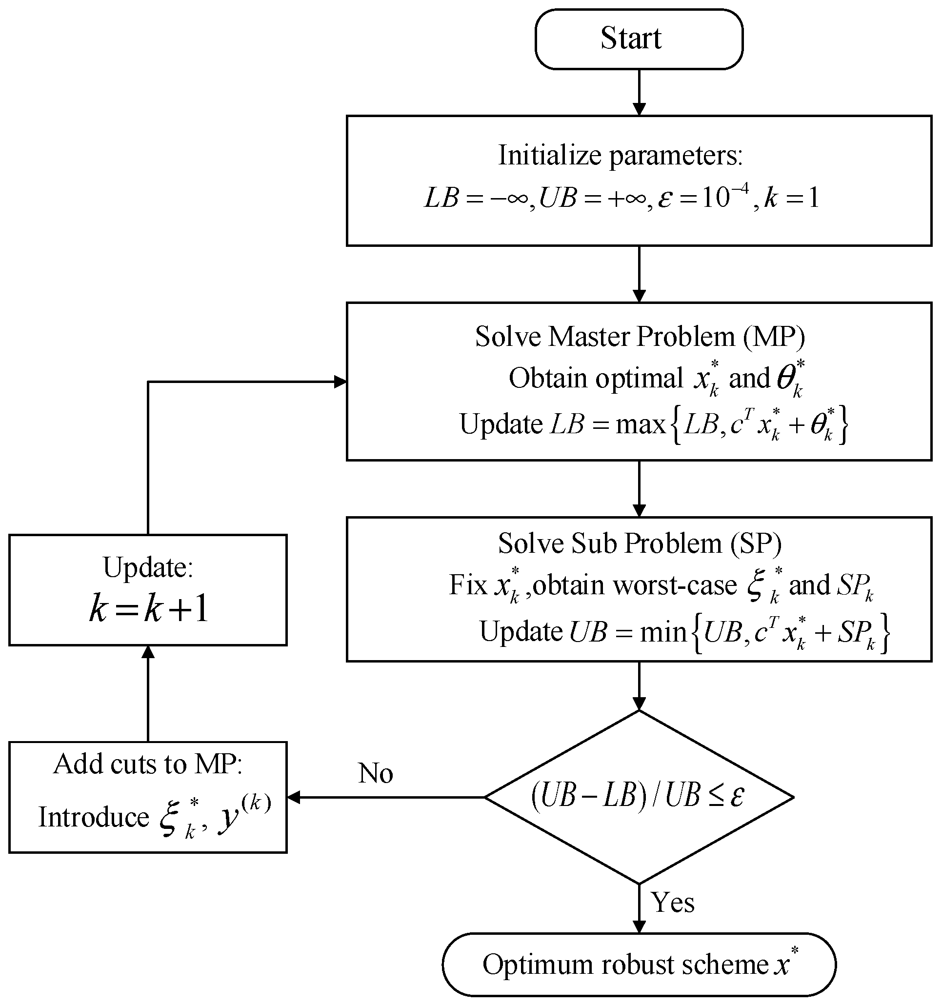
To solve the min–max–min structure of the proposed two-stage robust optimization model, a standard C&CG framework is adopted. It should be noted that C&CG is used here as a solution technique rather than as a methodological contribution of this paper. The main modeling contributions lie in the coordinated frequency-security constraints and the time-correlated uncertainty set introduced in the previous sections. The algorithm decomposes the original problem into a master problem and a subproblem in MILP format. Through alternating iterations between the master problem and the subproblem, and by adding the identified worst-case scenarios as cutting planes, the robust scheduling scheme satisfying the worst-case boundaries is obtained.

The master problem aims to find the optimal baseline scheduling and reserve pre-allocation scheme under the set of identified worst-case scenarios, providing a lower bound (LB) for the objective function. In the k-th iteration, the compact matrix form of the master problem is expressed as

$$\left\{\begin{array}{c}{}_{x,\theta }{}^{min}c^{T}x+\theta \\ \begin{array}{c}s.t. Ax\le d\\ \theta \ge f^T{y}^{\left(l\right)}, \forall l=1,2,\dots ,k\\ B{y}^{\left(l\right)}\le Ex+g-C{\xi }^{{\left(l\right)}^{*}}, \forall l=1,2,\dots ,k\end{array}\end{array}\right.$$

(55)

where $\theta$ is an auxiliary decision variable used to approximate the re-scheduling cost of the second-stage worst-case scenario; l is the current iteration index; ${\xi }^{{\left(l\right)}^{*}}$ is the extreme temporal disturbance scenario identified by the subproblem in the l-th iteration; and $y^{\left(l\right)}$ represents the re-scheduling decision variables newly generated for that specific scenario. After solving the master problem, the optimal day-ahead decision variables $x^{*}$ are passed to the inner subproblem.

The subproblem receives the optimal day-ahead decisions $x^{*}$ and identifies the worst-case scenario $\xi$ within the uncertainty set U that maximizes the system’s re-scheduling cost, thereby providing an upper bound (UB) for the objective function. Given $x^{*}$, the subproblem presents a max–min bi-level structure:

$$\left\{\begin{array}{c}SP\left(x^{*}\right)=\underset{\xi \in U}{max} \underset{y}{min}{f}^{T}y\\ s.t. By\le E{x}^{*}+g-C\xi :\mu \end{array}\right.$$

(56)

where $SP\left(x^{*}\right)$ is the objective value of the subproblem under the current iteration, and $\mu$ is the column vector of non-positive dual variables corresponding to the second-stage operational constraints.

By utilizing strong duality theory, the inner minimization problem is transformed into its equivalent maximization dual problem, thus merging the bi-level subproblem into a single-level maximization model:

$$\left\{\begin{array}{c}\hfill SP\left(x^{*}\right)={}_{\xi \in U,\mu \le 0}{}^{max}\mu ^T\left(E{x}^{*}+g\right)-{\mu }^{T}C\xi \hfill \\ \hfill s.t. B^T\mu \le f\hfill \end{array}\right.$$

(57)

As shown in Equation (57), the objective function contains a linear term ${\mu }^T\left(E{x}^{*}+g\right)$ and a bilinear non-convex term $-{\mu }^{T}C\xi$, which involves the product of continuous dual variables $\mu$ and uncertainty disturbance variables $\xi$. These bilinear terms represent the product of continuous and binary variables, which can be exactly linearized using the big-M method. Taking the dual product term related to PV disturbance as an example, a continuous auxiliary variable $w_{PV,t}={\mu }_t{u}_{PV,t}$ is introduced, and the following linear inequality constraints are added for equivalent substitution:

$$\left\{\begin{array}{c}-M{u}_{PV,t}\le w_{PV,t}\le M{u}_{PV,t}\\ {\mu }_t-M\left(1-u_{PV,t}\right)\le w_{PV,t}\le {\mu }_t+M(1-u_{PV,t})\end{array}\right.$$

(58)

where M denotes the upper bound used to linearize the product between the continuous dual expression and the binary uncertainty variable. In the numerical implementation, M is not selected as an arbitrarily large constant. Instead, it is determined according to the maximum marginal penalty coefficient in the second-stage re-scheduling problem.

An auxiliary emergency slack variable is introduced in the real-time re-scheduling model to guarantee complete recourse and prevent infeasibility under extreme uncertainty realizations. This slack variable is not regarded as a normal physical regulation resource; therefore, it is assigned the highest unit penalty coefficient, which is larger than the cost coefficients of all other second-stage recourse actions. The dual expressions associated with the PV and load uncertainty terms represent the marginal recourse costs caused by PV shortfall and load increase. Hence, their economically meaningful ranges are bounded by the maximum marginal penalty in the recourse problem. Accordingly, the Big-M value is set to be equal to the unit penalty coefficient of the auxiliary emergency slack variable in the numerical implementation.

Compared with using an excessively large big-M value, this cost-coefficient-based bound is consistent with the scale of the optimization model and helps avoid unnecessary numerical deterioration in Gurobi while preserving the exactness of the binary-continuous linearization.

When an extreme disturbance occurs ($u_{PV,t}=1$), $w_{PV,t}$ is strictly equal to ${\mu }_t$; when there is no disturbance ($u_{PV,t}=0$), $w_{PV,t}$ is strictly equal to 0. Similar linearization is applied to the bilinear terms involving load disturbances. After big-M linearization, the subproblem is thoroughly converted into a standard single-level MILP model, which can be efficiently solved by commercial solvers. The iterative C&CG solution process for the coordinated RO model is illustrated in Figure 1.

5. Case Study

5.1. Simulation Setup

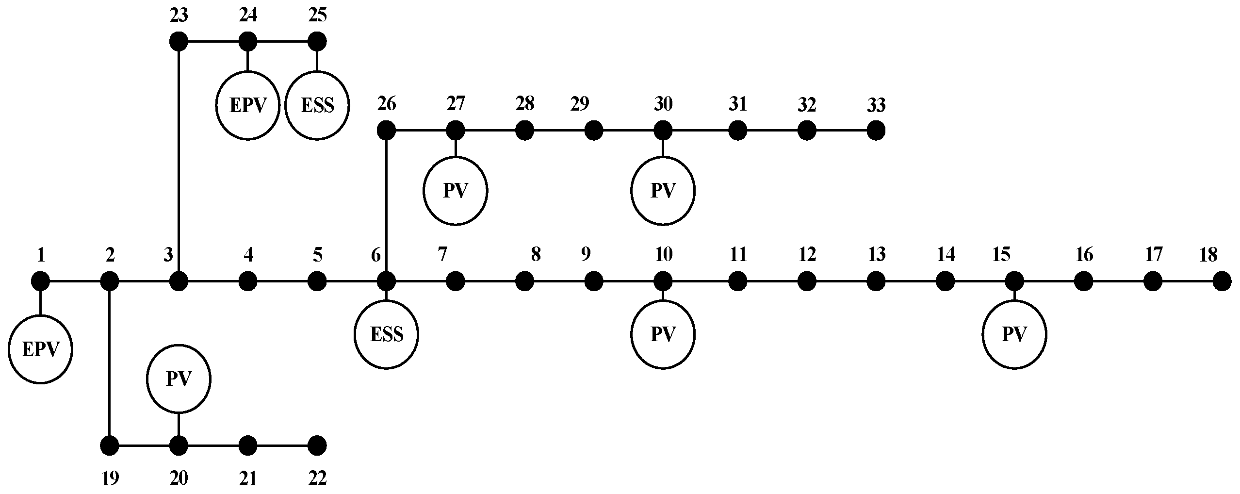
To verify the effectiveness of the proposed coordinated robust scheduling strategy, a modified IEEE 33-node system is utilized as the test topology for the temporary islanded microgrid, as illustrated in Figure 2.

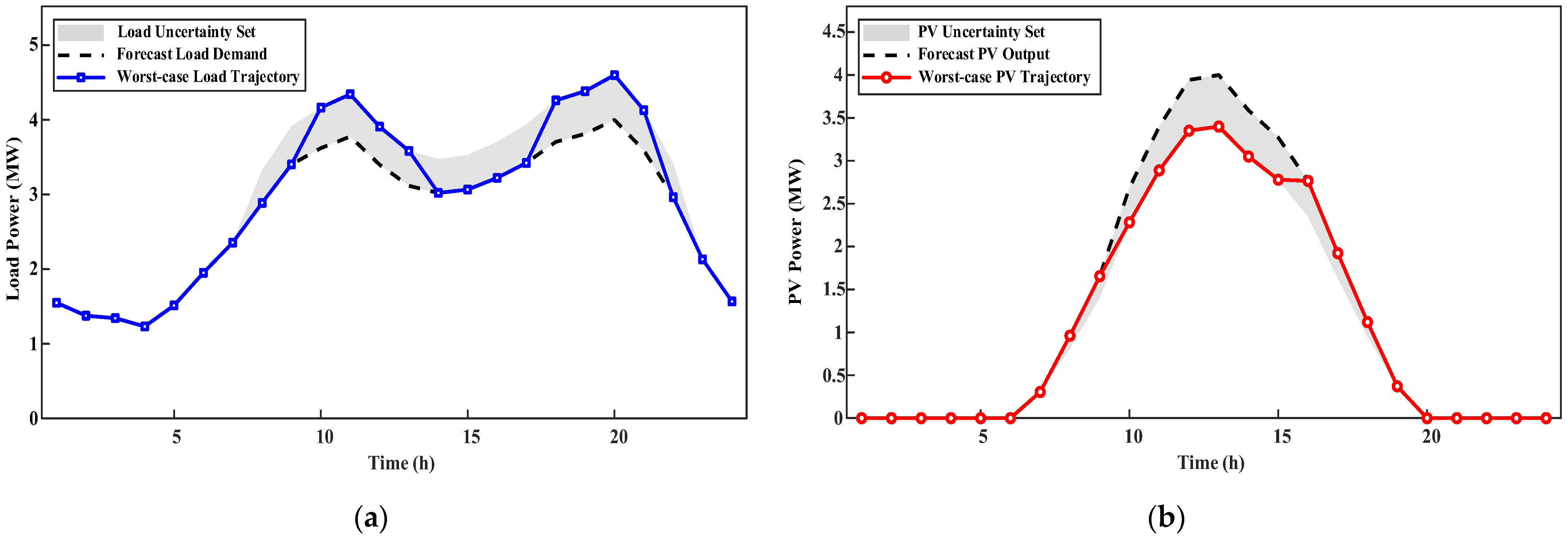
The baseline peak load of the islanded microgrid is 4.0 MW, and the total installed capacity of distributed PV is 4.0 MW. The rated operating frequency of the system is 50 Hz. The system power base is 10 MVA. To ensure transient stability during the islanded period, the maximum allowable RoCoF is set to 1.0 Hz/s, and the maximum allowable transient frequency nadir deviation is 0.8 Hz. In this study, the fluctuation deviations for both load power and PV output are considered to be 15% of their forecasted values. The forecasted/actual load power curves and PV output curves are shown in Figure 3, where the shaded areas represent the uncertainty sets considered in this paper. This study is developed on the MATLAB R2024a platform, modeled using YALMIP, and solved using the Gurobi solver.

To validate the advantages of the proposed model in constructing frequency defense lines and its adaptability to uncertain environments, the following four scheduling scenarios are established for comparative analysis.

Scenario 1 (Deterministic Scheduling): Source-load prediction errors are ignored, and the system does not pre-allocate robust reserve capacity to cope with sudden disturbances.

Scenario 2 (Rigid Frequency-Constrained RO): Source-load uncertainties and dynamic frequency security constraints are considered, but the virtual inertia coordination of the GFM-ESS is neglected, relying solely on the mechanical inertia of the EPVs.

Scenario 3 (Traditional Static RO): GFM-ESS virtual inertia coordination is considered, but the uncertainty set adopts the traditional static box model.

Scenario 4 (Proposed Scheduling Model): GFM-ESS virtual inertia coordination is considered, and the temporal-correlated uncertainty set is adopted.

5.2. Results and Analysis

The simulation results are presented according to the main objectives of the proposed model. Section 5.2.1 analyzes the power balance and demand response under the worst-case disturbance to verify the feasibility of the real-time recourse strategy. Section 5.2.2 compares Scenario 2 and Scenario 4 to demonstrate the economic and frequency-security benefits of GFM-ESS virtual inertia. Section 5.2.3 verifies the effectiveness of the time-correlated uncertainty set through worst-case trajectory comparison and budget sensitivity analysis. Section 5.2.4 further evaluates the robustness of the proposed scheduling scheme under different prediction-error levels.

5.2.1. Power Balance and Demand Response Under the Worst-Case Scenario

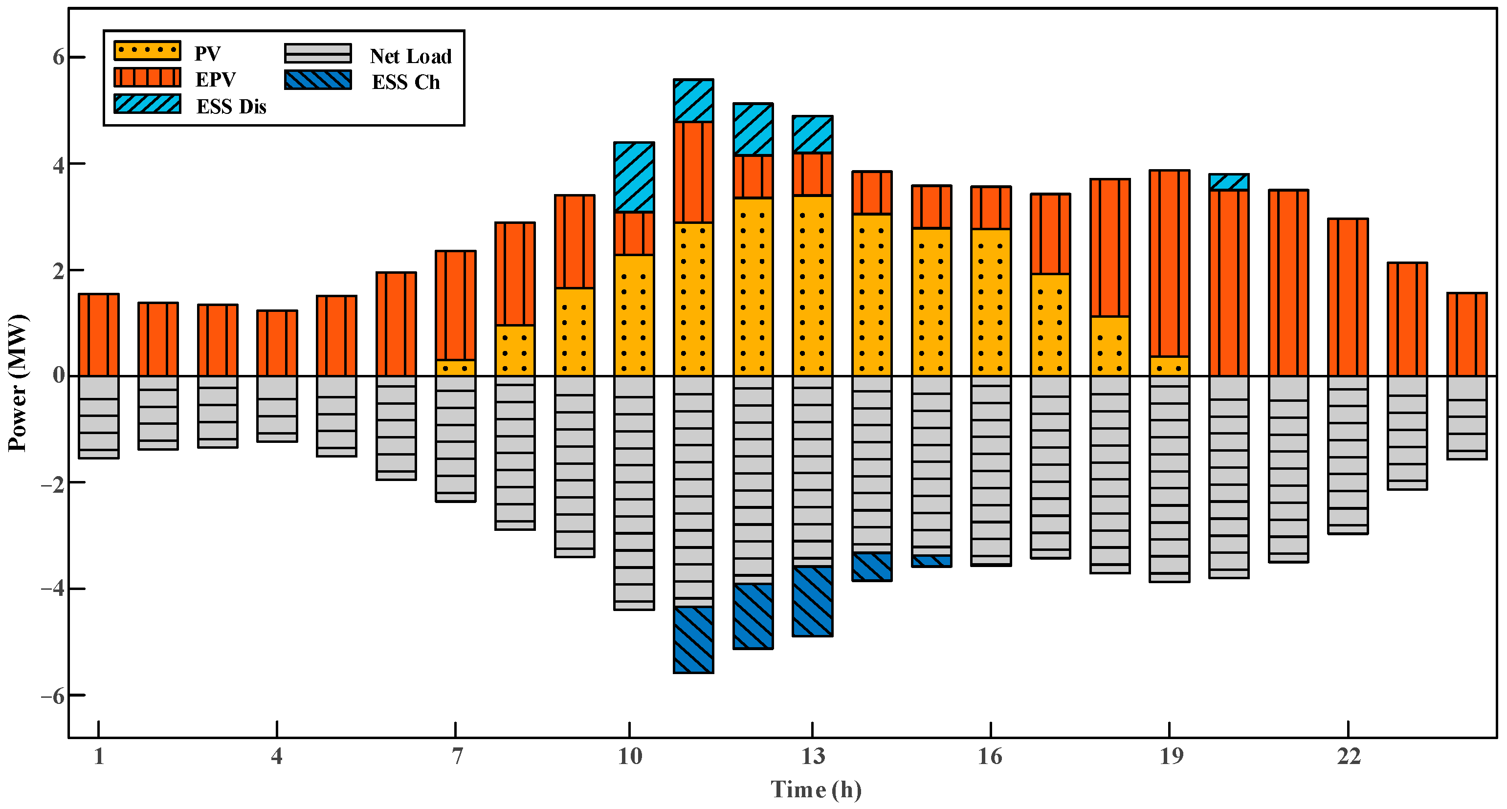
Using the coordinated robust scheduling strategy proposed in this paper, the overall power balance of the system when encountering the worst-case uncertainty disturbance is shown in Figure 4. In the islanded operation mode, the system loses main grid support, and its steady-state energy balance is primarily maintained by EPVs and distributed PV. The simulation results indicate that during the daytime PV peak period, the system prioritizes PV accommodation to reduce fuel costs; conversely, during the morning and evening net load peak periods, the two EPV units are dispatched to high output states to provide stable active power support.

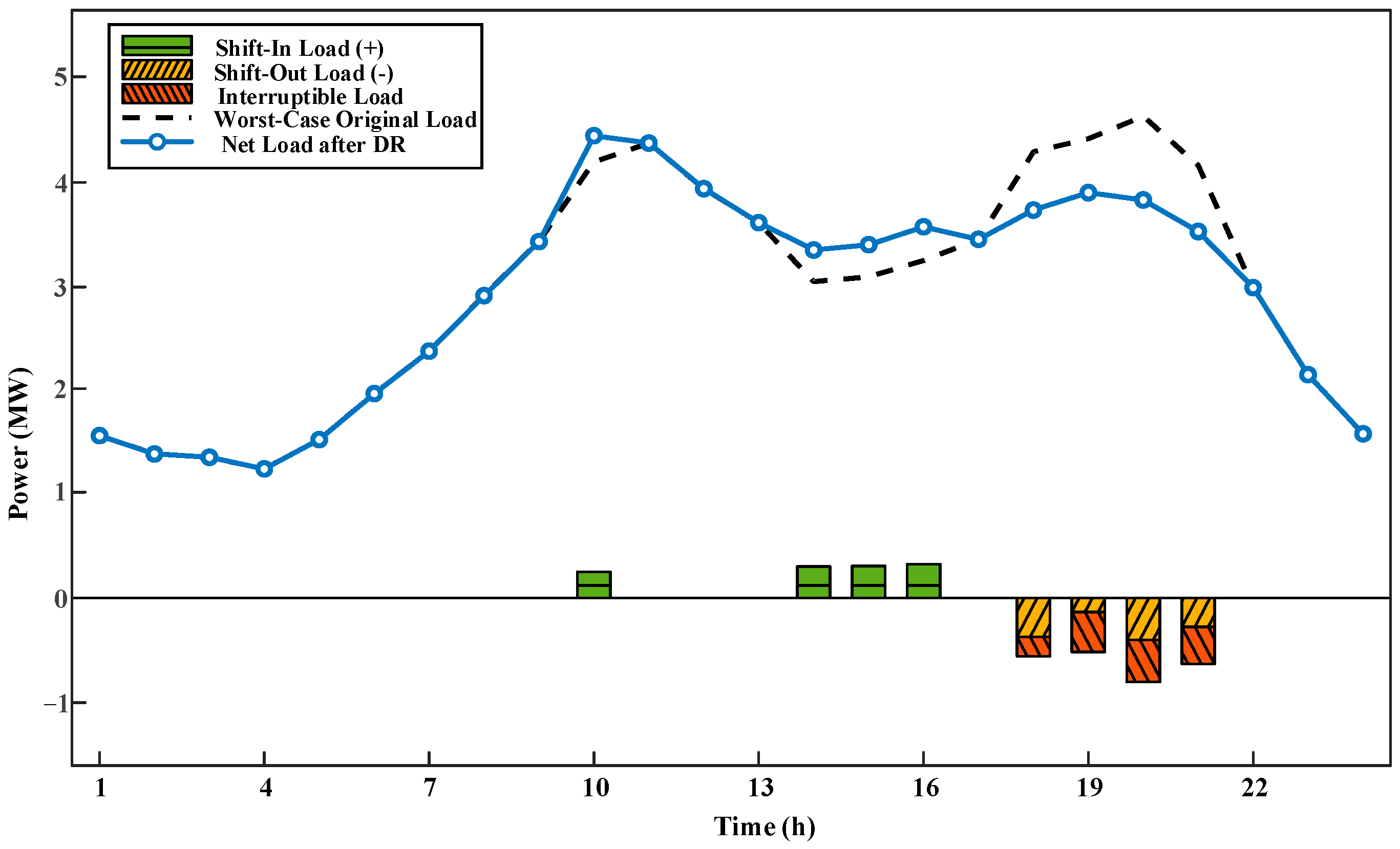
Between 10:00 and 14:00, when PV fluctuations are severe, the GFM-ESS switches between charging and discharging states to absorb extreme impacts and provide virtual inertia, compensating for the weak physical inertia of the system caused by the low-load operation of the EPVs. During the evening load peak period, the GFM-ESS does not discharge on a large scale. Due to the potential risk of extreme unidirectional disturbances during the evening peak, the scheduling model restricts the available energy of the storage, ensuring it maintains the physical capability to release maximum frequency regulation reserves and baseline virtual inertia at any time to prevent transient frequency collapse. While the storage is in a reserve state, the steady-state power deficit at the extreme boundary is regulated by flexible loads. As shown in Figure 5, SLs transfer partial peak demand to off-peak or PV accommodation periods. Simultaneously, at the critical nodes with the most severe power deficits, ILs are curtailed to ensure the system’s power balance without triggering extreme physical load shedding.

These results indicate that the proposed two-stage scheduling model can maintain the steady-state power balance under the worst-case disturbance by coordinating EPV output, GFM-ESS charging/discharging, PV curtailment, and flexible-load response. In particular, flexible loads are activated only during critical deficit periods, which helps avoid large-scale forced physical load shedding while preserving the frequency-security margin.

5.2.2. Frequency-Security Enhancement of GFM-ESS Virtual Inertia

To quantify the contribution of GFM-ESS virtual inertia to transient frequency stability, Scenario 2 and Scenario 4 are compared in

Table 1. Comparison of economic and security performance between Scenario 2 and Scenario 4.

Scheduling Scenario	EPV Operation Cost (CNY)	ESS Operation Cost (CNY)	Flexible Load Compensation Cost (CNY)	Penalty Cost (CNY)	Total Operation Cost (CNY)
Scenario 2	56,365.67	1700.45	2163.26	149,403.17	209,632.55
Scenario 4	63,946.43	3930.91	2056.68	535.17	70,469.18

. Scenario 2 relies only on the mechanical inertia of EPVs, whereas Scenario 4 coordinates EPV mechanical inertia with GFM-ESS virtual inertia. Since only two EPVs are deployed in the test system, the available mechanical inertia has a limited physical upper bound. Therefore, this comparison is used to evaluate whether the additional virtual inertia provided by the GFM-ESS can reduce emergency physical load shedding and improve the overall economic performance under extreme disturbances.

As shown in Table 1, Scenario 2 has a total operation cost of CNY 209,632.55, mainly because the lack of virtual inertia forces the system to trigger emergency physical load shedding, resulting in a penalty cost of CNY 149,403.17. In contrast, Scenario 4 reduces the total operation cost to CNY 70,469.18, corresponding to a 66.38% reduction. More importantly, the penalty cost decreases sharply from CNY 149,403.17 to CNY 535.17. Although Scenario 4 increases the EPV operation cost and ESS operation cost because more resources are maintained for frequency defense, this additional cost is economically justified by the substantial reduction in emergency load-shedding penalties.

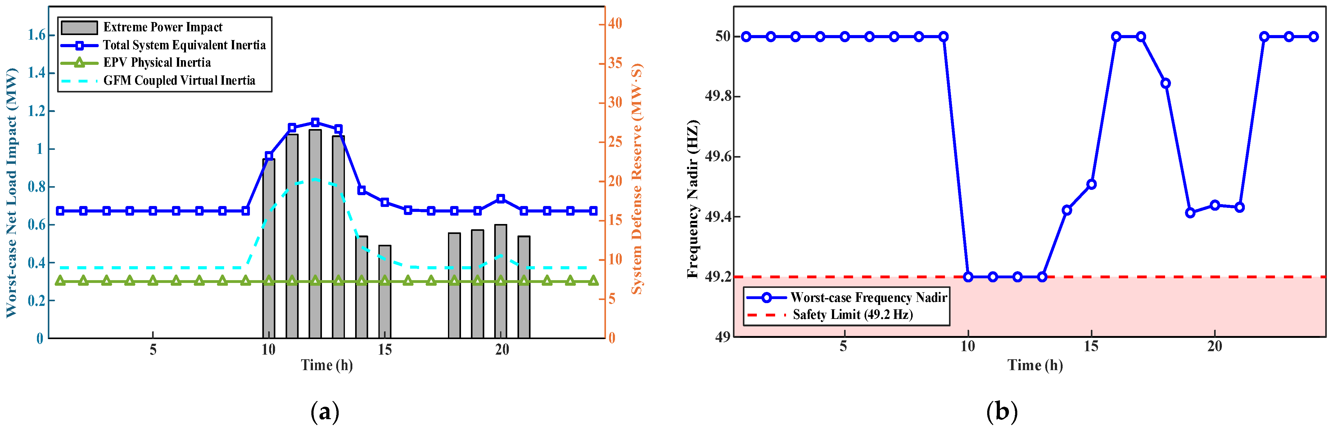
Figure 6 further explains the frequency-security mechanism behind the economic improvement. When the worst-case disturbance occurs, the total equivalent inertia is jointly provided by the EPV mechanical inertia and the GFM-ESS virtual inertia. The GFM-ESS increases the available inertia during the critical disturbance periods, thereby reducing the frequency drop caused by the power deficit. As a result, the worst-case frequency nadir is maintained above the safety threshold of 49.2 Hz throughout the scheduling horizon.

Therefore, the frequency-security constraints are not only feasible in the optimization model but also effective in the simulated worst-case scenario. The coordinated inertia provided by EPVs and GFM-ESSs enables the system to satisfy both RoCoF and frequency-nadir requirements.

5.2.3. Effectiveness of the Time-Correlated Uncertainty Set

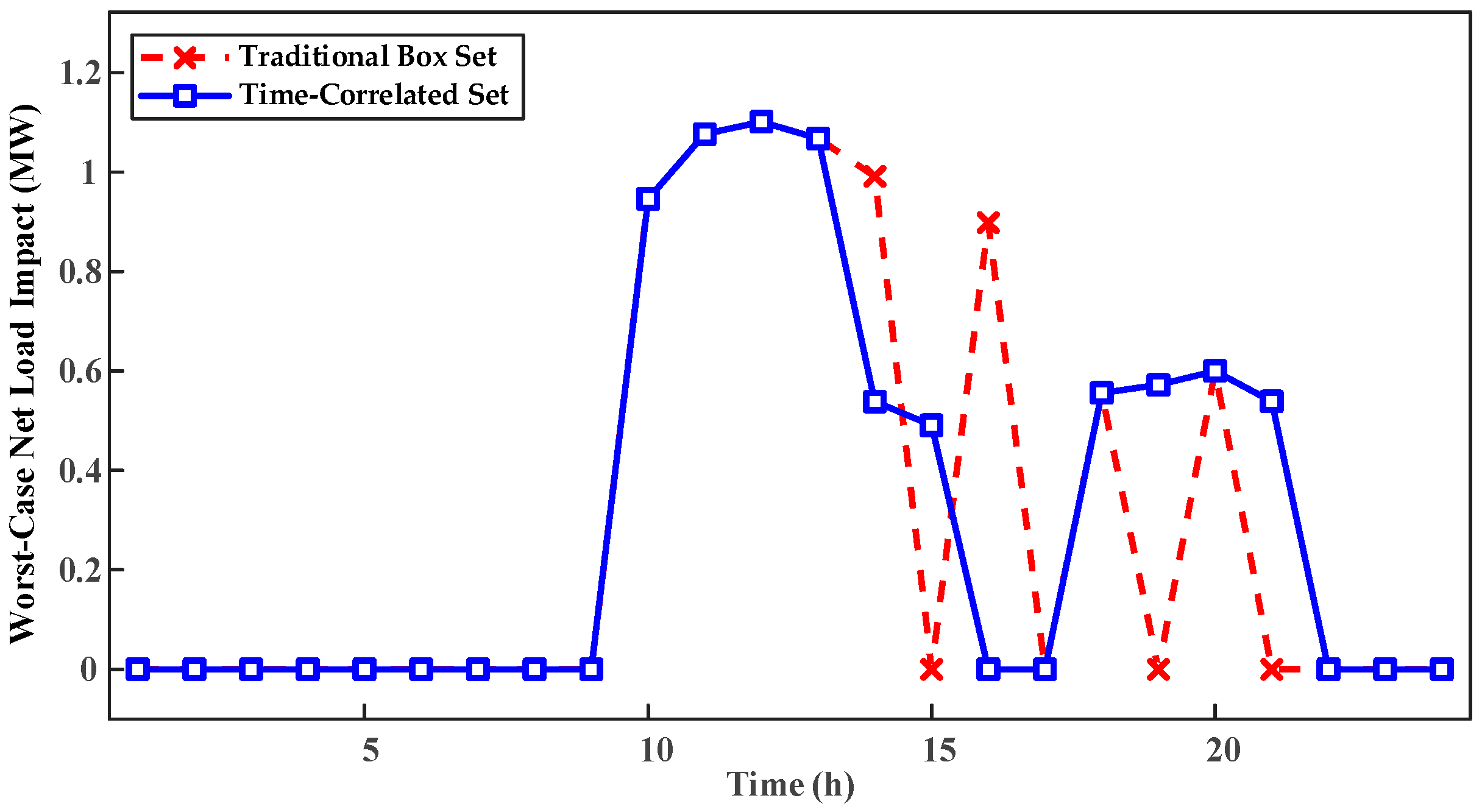
Addressing the conservatism of traditional static box uncertainty sets, Figure 7 shows that the box set in Scenario 3 generates a high-frequency alternating trajectory with a severe sawtooth pattern. Such non-physical step conditions have extremely low probabilities in actual meteorology and cause severe oscillations in the bi-level optimization. The proposed time-correlated uncertainty set mathematically filters these trajectories through temporal budget constraints, making the worst-case disturbance sequence more consistent with real weather patterns and enhancing solving efficiency. This comparison indicates that the improvement is not achieved by simply reducing the spatial uncertainty budget. Instead, the proposed temporal budget reshapes the admissible uncertainty trajectories by limiting the number of adjacent-period state transitions, thereby maintaining the disturbance-intensity level while excluding unrealistic high-frequency switching patterns.

To verify that the proposed optimization method can flexibly adjust the conservatism of the scheduling scheme, sensitivity analyses were conducted on the spatial uncertainty budget and the temporal budget, respectively. The parameter settings and corresponding operation costs are shown in

Table 2. Microgrid operation costs under different spatial uncertainty budgets.

Spatial Uncertainty Budget Γ	Total System Operation Cost (CNY)
ΓPV = 0, Γload = 0	56,626.46
ΓPV = 4, Γload = 6	67,259.74
ΓPV = 6, Γload = 9	70,469.18
ΓPV = 8, Γload = 12	75,597.79

and

Table 3. Microgrid operation costs and iteration counts under different temporal uncertainty budgets.

Temporal Budget Ψ	Total System Operation Cost (CNY)	Iteration Count
ΨPV = 2, Ψload = 2	70,005.85	7
ΨPV = 4, Ψload = 4	70,469.18	10
ΨPV = 6, Ψload = 6	70,607.03	18
ΨPV = 8, Ψload = 8	70,619.94	19

.

As shown in Table 2, when the spatial uncertainty budget increases from Γ_PV = 0, Γ_load = 0 to Γ_PV = 8, Γ_load = 12, the total operation cost increases from CNY 56,626.46 to CNY 75,597.79. This result indicates that a larger spatial budget expands the range of admissible severe source-load disturbances. Consequently, the system must reserve more generation capacity, flexible response capability, and virtual inertia, leading to higher scheduling conservatism and operation cost.

Table 3 shows that relaxing the temporal budget from Ψ_PV = 2, Ψ_load = 2 to Ψ_PV = 8, Ψ_load = 8 only slightly increases the total operation cost from CNY 70,005.85 to CNY 70,619.94, whereas the iteration count rises sharply from 7 to 19. This indicates that high-frequency switching trajectories mainly increase the computational burden of the C&CG process, while contributing limited additional economic conservatism. Therefore, the proposed temporal budget is not equivalent to simply reducing the spatial uncertainty budget; instead, it controls the temporal continuity of disturbance trajectories and filters out physically unlikely high-frequency switching patterns.

5.2.4. Robustness Under Different Prediction Errors

To evaluate the robustness of the proposed scheduling scheme against real-time prediction errors, deterministic scheduling and the proposed coordinated robust scheduling are compared under actual prediction errors ranging from 0% to 20%. Since the uncertainty boundary in the base case is set to 15% of the forecasted PV and load values, the 0–15% cases are used to verify the robustness within the predefined uncertainty boundary, while the 20% case is used as an out-of-boundary stress test. The final operation costs and forced load shedding amounts are shown in

Table 4. Performance comparison between deterministic scheduling and the proposed robust scheduling under different prediction errors.

Error Level	Scenario 1		Scenario 4
	Forced Load Shedding (MW)	Total Cost (CNY)	Forced Load Shedding (MW)	Total Cost (CNY)
0%	0.00	55,627	0.00	68,349
5%	0.37	102,975	0.01	69,056
10%	0.73	168,783	0.01	69,763
15%	1.10	243,649	0.02	70,469
20%	1.47	318,516	0.37	145,335

.

The comparison indicates that deterministic scheduling is highly sensitive to prediction errors because it does not pre-allocate sufficient reserve headroom and virtual inertia. Even at the 5% prediction-error level, Scenario 1 requires 0.37 MW of forced load shedding, and the total operation cost increases to CNY 102,975. As the prediction error increases to 15%, the forced load shedding of Scenario 1 reaches 1.10 MW, and the total operation cost rises to CNY 243,649.

In contrast, the proposed robust scheduling model demonstrates stronger disturbance rejection capability within the predefined uncertainty boundary. At the 15% prediction-error level, Scenario 4 limits forced load shedding to 0.02 MW, whereas Scenario 1 requires 1.10 MW of forced load shedding. Meanwhile, the total operation cost of Scenario 4 is CNY 70,469, which is much lower than the CNY 243,649 of Scenario 1. This result shows that the proposed model can effectively reserve sufficient inertia and frequency-response resources to withstand source-load prediction errors within the predefined robust boundary.

When the prediction error increases to 20%, which exceeds the predefined robust boundary, Scenario 4 also experiences forced load shedding because the reserved frequency-response resources are partially depleted. Nevertheless, Scenario 4 reduces forced load shedding from 1.47 MW in Scenario 1 to 0.37 MW and reduces the total operation cost from CNY 318,516 to CNY 145,335. This out-of-boundary stress-test result indicates that the proposed scheme still provides a stronger resilience margin than deterministic scheduling, although its full robustness guarantee is designed for the predefined 15% uncertainty boundary.

6. Conclusions

Addressing the frequency security issues of islanded microgrids under extreme conditions, this paper proposes a two-stage coordinated robust optimization scheduling model incorporating dynamic frequency constraints and virtual inertia. Based on the case studies, the following main conclusions are drawn:

(1)

The proposed model achieves the coordinated optimal configuration of the physical mechanical inertia from EPVs and the virtual inertia from the GFM-ESS. Through two-stage robust optimization, the microgrid can attain both economic operation and transient frequency security under “worst-case” disturbance scenarios by pre-allocating an adequate dynamic inertia defense line.

(2)

To address the limitation of traditional box uncertainty sets that ignore temporal continuity, the proposed time-correlated uncertainty set introduces temporal state-transition budgets in addition to conventional spatial uncertainty budgets. The spatial budget determines the number of disturbed periods, whereas the temporal budget limits the number of adjacent-period state transitions. Therefore, the proposed uncertainty set can filter out non-physical high-frequency oscillation trajectories and generate worst-case scenarios that are more consistent with continuous severe-weather evolution.

(3)

By adjusting the spatial uncertainty budget and the temporal budget, dispatchers can flexibly trade off operational economy against defensive conservatism. Increasing the budgets raises the costs of reserving capacity and inertia but enhances the microgrid’s capability to cope with extreme continuous disturbances, facilitating rational decision-making between operation costs and risks.

(4)

The proposed scheme substantially reduces forced load shedding and maintains the supply of critical loads within the predefined robust uncertainty boundary. Even when the prediction error exceeds the predefined boundary, the proposed scheme still significantly mitigates the affected load compared with deterministic scheduling.

References

1. Panteli, M.; Mancarella, P. Influence of Extreme Weather and Climate Change on the Resilience of Power Systems: Impacts and Possible Mitigation Strategies. Electr. Power Syst. Res. 2015, 127, 259–270. [Google Scholar] [CrossRef] [Scilit]
2. Wang, Y.; Rousis, A.O.; Strbac, G. On Microgrids and Resilience: A Comprehensive Review on Modeling and Operational Strategies. Renew. Sustain. Energy Rev. 2020, 134, 110313. [Google Scholar] [CrossRef] [Scilit]
3. Chen, C.; Wang, J.; Qiu, F.; Zhao, D. Resilient Distribution System by Microgrids Formation After Natural Disasters. IEEE Trans. Smart Grid 2016, 7, 958–966. [Google Scholar]
4. Lei, S.; Chen, C.; Zhou, H.; Hou, Y. Routing and Scheduling of Mobile Power Sources for Distribution System Resilience Enhancement. IEEE Trans. Smart Grid 2019, 10, 5650–5662. [Google Scholar]
5. Milano, F.; Dörfler, F.; Hug, G.; Hill, D.J.; Verbič, G. Foundations and Challenges of Low-Inertia Systems (Invited Paper). In Proceedings of the 2018 Power Systems Computation Conference (PSCC); IEEE: New York, NY, USA, 2018; pp. 1–25. [Google Scholar]
6. Tielens, P.; Van Hertem, D. The Relevance of Inertia in Power Systems. Renew. Sustain. Energy Rev. 2016, 55, 999–1009. [Google Scholar] [CrossRef] [Scilit]
7. Zhong, Q.-C. Virtual Synchronous Machines: A Unified Interface for Grid Integration. IEEE Power Electron. Mag. 2016, 3, 18–27. [Google Scholar] [CrossRef] [Scilit]
8. Fang, J.; Li, H.; Tang, Y.; Blaabjerg, F. On the Inertia of Future More-Electronics Power Systems. IEEE J. Emerg. Sel. Top. Power Electron. 2019, 7, 2130–2146. [Google Scholar]
9. Gu, H.; Yan, R.; Saha, T.K. Minimum Synchronous Inertia Requirement of Renewable Power Systems. IEEE Trans. Power Syst. 2018, 33, 1533–1543. [Google Scholar]
10. Markovic, U.; Chu, Z.; Aristidou, P.; Hug, G. LQR-Based Adaptive Virtual Synchronous Machine for Power Systems with High Inverter Penetration. IEEE Trans. Sustain. Energy 2019, 10, 1501–1512. [Google Scholar]
11. Qoria, T.; Gruson, F.; Colas, F.; Guillaud, X.; Debry, M.-S.; Prevost, T. Tuning of Cascaded Controllers for Robust Grid-Forming Voltage Source Converter. In Proceedings of the 2018 Power Systems Computation Conference (PSCC); IEEE: New York, NY, USA, 2018; pp. 1–7. [Google Scholar]
12. Badesa, L.; Teng, F.; Strbac, G. Simultaneous Scheduling of Multiple Frequency Services in Stochastic Unit Commitment. IEEE Trans. Power Syst. 2019, 34, 3858–3868. [Google Scholar] [CrossRef] [Scilit]
13. Chapaloglou, S.; Alves, E.F.; Trovato, V.; Tedeschi, E. Optimal Energy Management in Autonomous Power Systems With Probabilistic Security Constraints and Adaptive Frequency Control. IEEE Trans. Power Syst. 2024, 39, 1543–1554. [Google Scholar] [CrossRef] [Scilit]
14. Tian, Y.; Li, Z.; Wu, W.; Fan, M. Joint Chance-Constrained Economic Dispatch Involving Joint Optimization of Frequency-Related Inverter Control and Regulation Reserve Allocation. CSEE J. Power Energy Syst. 2025, 11, 1030–1044. [Google Scholar]
15. Xiang, Y.; Liu, J.; Liu, Y. Robust Energy Management of Microgrid With Uncertain Renewable Generation and Load. IEEE Trans. Smart Grid 2015, 7, 1. [Google Scholar] [CrossRef] [Scilit]
16. Li, X.; Liu, Y.; Guo, L.; Li, X.; Wang, C. Data-driven Based Uncertainty Set Modeling Method for Microgrid Robust Optimization with Correlated Wind Power. CSEE J. Power Energy Syst. 2023, 9, 420–432. [Google Scholar] [CrossRef] [Scilit]
17. Yang, X.; Li, Y.; Zhao, Y.; Yu, Y.; Lian, Y.; Hao, G.; Jiang, L. Data-Driven Nested Robust Optimization for Generation Maintenance Scheduling Considering Temporal Correlation. Energy 2023, 278, 127499. [Google Scholar] [CrossRef] [Scilit]
18. Lorca, A.; Sun, X.A. Multistage Robust Unit Commitment With Dynamic Uncertainty Sets and Energy Storage. IEEE Trans. Power Syst. 2017, 32, 1678–1688. [Google Scholar]
19. Zheng, Z.; Chen, G.; Shen, Z. Interval-Partitioned and Correlated Uncertainty Set Based Robust Optimization of Microgrid. IEEE Syst. J. 2024, 18, 1516–1527. [Google Scholar] [CrossRef] [Scilit]
20. Tang, Z.; Liu, J.; Liu, Y.; Xu, L. Stochastic Reserve Scheduling of Energy Storage System in Energy and Reserve Markets. Int. J. Electr. Power Energy Syst. 2020, 123, 106279. [Google Scholar] [CrossRef] [Scilit]
21. Chen, J.; Liu, M.; Milano, F.; O’Donnell, T. Adaptive Virtual Synchronous Generator Considering Converter and Storage Capacity Limits. CSEE J. Power Energy Syst. 2022, 8, 580–590. [Google Scholar]
22. Fan, H.; Wang, H.; Xu, Y.; Hu, J.; Zhang, W.; Xiao, X. Capacity Value Analysis of Interruptible Loads in Regional Power Systems with Intermittent Renewable Energy. Front. Energy Res. 2022, 10, 968873. [Google Scholar] [CrossRef] [Scilit]
23. Mathur, A.; Nema, S.; Prakash, V.; Singh, J. Fast Frequency Response Constrained Stochastic Scheduling of Flexible Loads in Low Inertia Grids. e-Prime-Adv. Electr. Eng. Electron. Energy 2024, 10, 100852. [Google Scholar] [CrossRef] [Scilit]
24. Wu, H.; Xie, Y.; Li, H.; Wu, Q.; Yu, C.; Sun, J. Robust Load Restoration Optimization of Power System Considering the Spatial-Temporal Correlation of Wind Power. Int. J. Electr. Power Energy Syst. 2023, 147, 108855. [Google Scholar]
25. Lorca, A.; Sun, X.A. Adaptive Robust Optimization with Dynamic Uncertainty Sets for Multi-Period Economic Dispatch under Significant Wind. IEEE Trans. Power Syst. 2015, 30, 1702–1713. [Google Scholar]
Figure 1. Flowchart of C&CG.
Electricity 07 00064 g001
Figure 2. Topology of the modified IEEE 33-node system.
Electricity 07 00064 g002
Figure 3. Forecasted/actual curves: (a) load power demand; (b) PV output power.
Electricity 07 00064 g003
Figure 4. Power balance of the islanded microgrid system under the worst-case scenario.
Electricity 07 00064 g004
Figure 5. Flexible load demand response.
Electricity 07 00064 g005
Figure 6. Dynamic frequency security response: (a) system frequency defense line; (b) system frequency nadir under the worst-case scenario.
Electricity 07 00064 g006
Figure 7. Comparison of worst-case disturbance trajectories between the traditional box set and the proposed temporal-correlated uncertainty set.
Electricity 07 00064 g007