Abstract
To tackle the challenges arising from missing real-time measurement data and dynamic changes in network topology in optimizing and controlling distribution networks, this study proposes a data-driven collaborative optimization strategy tailored for multi-area clusters. Firstly, the distribution network is clustered based on electrical distance modularity and power balance indicators. Next, a collaborative optimization model for multiple area clusters is constructed with the objectives of minimizing node voltage deviations and active power losses. Then, a locally observable Markov decision model within the clusters is developed to characterize the relationship between the temporal operating states of the distribution network and the decision-making instructions. Using the Actor–Critic framework, the cluster agents are trained while considering the changes in cluster boundaries due to topology variations. A Critic network based on an attention encoder is designed to map the dynamically changing cluster observations to a fixed-dimensional space, enabling agents to learn control strategies under topology changes. Finally, case studies show the effectiveness and superiority of the proposed method.
1. Introduction
With the key progress of green energy low-carbon transformation, a large amount of distributed generation (DG) needs wide access to the distribution network. The future Active Distribution Network (ADN) is anticipated to transition from a traditional unidirectional radial configuration to a bidirectional active network. The control mode will be changed from centralized dispatch to hierarchical and clustered control, constituting a hybrid AC–DC distribution network with medium and low voltage interaction and multi-station interconnection. However, due to the large random volatility and strong uncertainty of DG output, which is typically represented by photovoltaic (PV) energy, leading to prominent problems such as voltage overruns and power imbalance in the distribution network, the challenge of new energy consumption is highlighted [1]. Therefore, fully utilizing adjustable resources to implement autonomous operation at the distribution level and collaborative optimization control across multiple distribution areas has become one of the effective means of addressing the aforementioned issues.
Currently, optimal regulation methods for ADN can be classified into two main categories: model-driven [2,3] and data-driven approaches [4]. The model-driven category typically employs mathematical planning methods and heuristic algorithms to formulate the optimal regulation problem of ADN as a nonlinear optimization problem that can be explicitly solved. However, the limited coverage of communication facilities in medium- and low-voltage distribution networks [5], along with frequent changes in line-switching states, results in issues such as incomplete real-time measurement data [6] and fluctuations in network topology. Consequently, the traditional model-driven approach, which relies on comprehensive measurement data, is becoming less applicable.
In recent years, as power grids have undergone intelligent upgrades, data-driven methods, particularly Deep Reinforcement Learning (DRL), have emerged as innovative solutions for the real-time optimization and regulation of distribution networks [6,7,8]. These approaches are leveraged to enhance decision-making processes in dynamic environments by large datasets and adaptive learning techniques.
DRL is essentially a framework of interaction-based learning that models control resources as intelligent agents within the distribution network environment. This integration allows for continuous interaction, enabling the system to learn from the vast amounts of operational data generated during these interactions. Neural networks are utilized to efficiently develop regulation strategies based on the acquired data. As the size of distribution network nodes and the penetration of photovoltaic (PV) systems increase, the expansion of control equipment results in a growing number of intelligent entities. However, this increase can lead to suboptimal synergistic effects among these entities [9]. Additionally, node voltage violations tend to occur in only a limited number of regions, indicating that it is unnecessary to mobilize all resources in order to address localized voltage fluctuations. To tackle these challenges, existing research has explored collaborative optimization of distribution network zones through clustering techniques in [10,11]. This approach aims to enhance the consumption of DG resources in close proximity. For instance, [12] proposes a dynamic clustering method based on a multi-scenario hierarchical clustering approach, which segments the distribution network into clusters. In this framework, intelligent agents are deployed within each region to undergo training, facilitating zonal in situ optimization and improving overall system performance.
However, the aforementioned DRL methods primarily focus on fixed network topologies, which do not account for the dynamic changes that occur in actual distribution networks due to load transfers and the opening and closing of switches. These changes inevitably affect cluster divisions and the dynamic assignment of regulation units to clusters, which involves determining which regulation units are in the same cluster and share regional information. In traditional DRL, the input network dimensions for each agent are fixed, i.e., as the power flow data of all agents within the same cluster at the distribution network nodes. However, when the cluster changes, it leads to changes in the input dimensions of the agent network, rendering traditional methods unsuitable. To address this issue, researchers have concentrated on two main areas: strategy transfer learning and topological feature learning.
In the realm of policy transfer learning, [13] utilized the migration capabilities of neural networks to transfer parameters of the policy network based on a pre-trained intelligent agent model under a specific topological structure. However, this policy transfer method is limited in that it acts merely as a refinement measure after a topology change event has occurred. It also assumes that the state space of the intelligent agent remains unchanged, which introduces certain constraints.
On the other hand, topological feature learning approaches, as discussed in [14,15,16,17], aim to characterize the regional topology of the distribution network using adjacency matrices or one-dimensional vectors. In these methods, neural networks learn the numerical variations of these matrices or vectors to identify anomalies in network topology. Nevertheless, constructing these matrices or vectors still requires a global understanding of the distribution network’s topology or of the entire cluster, which places high demands on the quality of the real-time communication infrastructure.
In summary, this paper presents a data-driven cooperative optimal regulation method designed for multiple area clusters, aimed at enhancing the adaptability of algorithms to changes in distribution network topology. The approach begins by segmenting the distribution network into clusters based on electrical distance modularity and power balance degree. This segmentation allows for the decomposition of the overall distribution network regulation problem into a series of intra-cluster autonomy issues.
Next, the optimization problem for the distribution network is modeled using sequential decision-making principles grounded in the Markov Decision Process (MDP). To address the dynamic nature of cluster boundaries resulting from topology changes, the paper introduces an attention-based Critic network. This network is designed to accommodate dynamic observations, enabling the inputs to the Critic network to be scalable in response to changing conditions.
Finally, the effectiveness and superiority of the proposed algorithms are rigorously evaluated and compared using the IEEE 33-bus test system.
2. Dynamic Clustering of Distribution Networks
The cluster segmentation metric serves as a foundational element for the aggregation of distribution areas, ensuring that clusters are formed in a way that promotes high electrical coupling within the clusters while maintaining approximate decoupling between them. In this paper, two primary indices are utilized for cluster division: electrical distance modularity and power balance.
Electrical Distance Module Degree Metric: The Module Degree is used to measure the strength of the community network structure; the larger the value of the Module Degree, the better the results of the cluster division [18]. The Module Degree function is defined as ρ:
where is the adjacency matrix in the modularity metric; is the sum of the weights of all edges connected to node i; s is the sum of the weights of all networks; denotes the cluster where station i is located, is a 0–1 function, and = 1 means that node i and node j are classified into a cluster. The formula for is given in [19].
Power Balance Degree Metric: In order to achieve full DG consumption and reduce the power outgoing from the cluster, a power balance degree metric e describing the balance between power supply and demand within the cluster is defined:
where is the total reactive power balance index of the system, and is the total active power balance index of the system. The active power balance index is used to describe the balance relationship between active power demand and supply within the cluster and can be expressed as
where is the net power characteristic of cluster s at time t; T is the duration of the typical time-varying scenario; and c is the number of clusters.
where , are the maximum reactive power output and reactive power demand of cluster s, respectively, and is the reactive power balance degree of cluster s.
Combining the modularity metric and power balance metric, the cluster composite division metric is expressed as
where a1 and a2 are the weighting coefficients of the two cluster indicators.
The distribution network is clustered into multiple area clusters by the Smart Local Moving (SLM) algorithm, which iteratively optimizes the cluster configuration to maximize modularity. Initially, each station area within the distribution network is treated as a distinct cluster. Subsequently, a sequential assignment process is employed, wherein each station area is evaluated for potential reassignment to a cluster containing other substation nodes. The modularity metric is calculated before and after each potential reassignment, and the node exhibiting the largest modularity increment is recorded. This process is repeated until the modularity converges, indicating a local optimum. The resulting clusters are then aggregated to form sub-networks, which are subsequently treated as nodes in a higher-level clustering iteration. This hierarchical clustering process continues until the modularity ceases to increase, thereby yielding an optimal division of the distribution network into multiple area clusters.
3. Co-Optimization Model for Multiple Area Clusters in Distribution Networks
3.1. Equivalent Power Modeling of Distribution Substation
The relationship between the LV distribution substation and the feeder connection is shown in Figure 1, where the station area internally interacts with the overall external active and reactive power at each moment with the feeder layer.
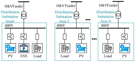
Figure 1.
Chained flexible interconnection structure with decentralized configuration of distribution substation.
The equipment such as PV, energy storage system (ESS), and DC load is included in the station, and the power balance equation for station i is
where and are the active and reactive power of DG flowing into station i, respectively; and are the charging and discharging power of energy storage, respectively; and are the active and reactive power of load in station i, respectively; and and are the active and reactive power flowing into the station, respectively.
3.2. Objective Functions
To fully leverage the regulatory capabilities of adjustable resources within the distribution substation area, a cooperative optimization model designed for multiple distribution stations is presented in this section. The primary objective of this model is to minimize both voltage deviation and active network loss in the distribution network. The model incorporates several critical constraints, including power balance, the operational limits of regulation resources, and voltage security at various nodes. By optimizing the reactive power output of photovoltaic (PV) systems and the charging and discharging power of energy storage systems (ESS), the model aims to enhance both the economic efficiency and operational security of the distribution network. Building upon the clustering results obtained in the preceding section, the scalar objective function is formulated as follows:
where is the number of the cluster; is the set of all clusters; denotes the set of nodes of cluster m; T denotes the total time period of the scheduling cycle; is the voltage amplitude of node i at time t, and is the voltage reference value; is the active network loss of cluster m at time t; is the set of branch circuits within cluster m; is the resistance of the branch circuit ij; and and are the inflow of active and reactive power into the branch circuit ij, respectively.
3.3. Constraints
- Distribution network power balance constraints
- Operational security constraints
- DG regulation performance constraints
PV active power uses the maximum power tracking mode (Maximum Power Point Tracking, MPPT); this paper considers the full consumption of distributed PV, but only its reactive capacity to regulate. The reactive power regulation range in constant apparent power control mode is
where is the maximum capacity of PV, is the active output of PV, and is the reactive output of PV.
The active power output range of PV system is expressed as
where represents the active power output under the maximum power point tracking control mode.
Meanwhile, The State of Charge (SOC) of the ESS at the current moment is related to the SOC state and charge/discharge power of the previous moment, and the ESS charge/discharge power constraint is
where denotes the power stored in the ESS in station i at time t, and are the ESS charging and discharging efficiencies, respectively, is the upper limit of the ESS storage power, is the ESS discharging state identifier, denotes that the ESS is in the discharging state, denotes that the ESS is in the charging state, and and denote the maximum values of the ESS charging and discharging power, respectively.
4. Model Optimal Solving Based on Deep Reinforcement Learning
4.1. Dynamic Clustering Markov Decision Process for Multiple Distribution Areas
The co-optimization of multiple areas within a distribution network involves decision-making that is informed by both the current and prior operating states, thereby characterizing it as a sequential decision-making problem. Given the weak electrical coupling between clusters following the clustering process, autonomous regulation is facilitated within each cluster. Consequently, this paper employs a Markov decision model of multiple intelligences to model the clusters of various station areas, treating each station area as an individual intelligence and the distribution network as the training environment. The principal components of the model are delineated as follows:
- Intelligent agent observation space
The observation space is defined as the set of observational variables that inform the decision-making process of the distribution area agent i. This includes critical parameters, such as the power and voltage measurements at the grid-connected nodes within the distribution area:
where and are the active and reactive power of the distribution network node connected to station i at time t.
- Intelligent agent state space
Intelligent agent observations of stations belonging to the same cluster constitute the environmental state of the distribution network, and the state space is represented as
where is the set of all station nodes in cluster m.
Considering that, after the topology changes as shown in Figure 2, the state space of each cluster intelligence also changes accordingly with the cluster boundary, taking the three station intelligences i1, i2 and i3 in topology A as examples, their state spaces are, respectively,
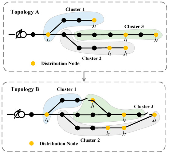
Figure 2.
Diagram of cluster boundary changes under different topologies.
When the topology is changed from A to B, then the state space of the three station intelligences at this time becomes, respectively,
- Intelligent agent action space
The action space represents the amount of decision making by the intelligent agent in the station based on the observation of , specifically:
where and are the active and reactive powers of station area i interacting with the feeder layer, which are realized by the station-side PV and storage inverters, respectively. denotes the active power emitted by the station, denotes the active power absorbed, and similarly.
After the execution of the action , the power of the distribution network node connecting station area i is
- Reward function
The reward function is used to measure the value of a set of observation–actions of an intelligent agent i. Rewards include objective function rewards and constraint rewards. The larger the reward function, the closer to the optimal goal under the current. The relationship between station areas is one of collaborative cooperation, and the reward function is expressed as the negative of the objective function combined with a penalty term:
where represents the constraint on the energy storage capacity that is infringed upon during the decision-making process associated with the action variables of intelligent agent j. is the weight coefficient for balancing the goal reward and the constraint reward, and , , and are the ESS penalty function coefficients.
- State transfer
After executing an action based on the current observation, the intelligent agent j obtains the timely reward function and enters the next state to achieve the observation of the next moment. This process is a state transfer, and the whole process starts from the initial moment and transfers states over time sections until there is no feasible solution for the trend or until the end of a scheduling cycle.
4.2. Model Solving Based on the Actor–Critic Framework
The decision variables of the distribution area agent are characterized by the active and reactive power outputs associated with DG and ESS, both of which are continuously adjustable, so the MADDPG algorithm is chosen to solve the continuous action behavior space in multi-intelligence reinforcement learning. For each intelligent agent i, the MADDPG algorithm needs to maintain four neural networks: the Actor network that executes an action based on observation and the target Actor network; the Critic network utilized to evaluate the value of actions and the target Critic network, where and denote the set of observations-actions of smart agent i and the rest of the intelligences in the same cluster at the time t, and are the corresponding parameters of the networks, respectively. The target network does not participate in the network training, and the parameters of the Actor and Critic networks are periodically copied to the corresponding target network to stabilize the network training process. The output of the Actor network is the action , denoted as
where is Gaussian noise, and is the upper and lower action limits, i.e., the upper and lower limits of the interaction power between the station and the distribution network; represents a random number between the upper and lower action limits.
The Critic network output is the value assessment for and , and the network parameters are updated based on gradient descent, the update formulae detailed in Section 4.3. The Actor network is trained using gradient ascent to maximize the value of current .
4.3. Attention Critic Network for Counting Dynamic State Quantity Inputs Under Cluster Changes
The Critic network of the traditional MADDPG algorithm consists of a fully connected neural network, where the number of neurons in the input layer corresponds to a fixed dimension of . Once the Critic network is constructed, its input dimensions cannot be modified, which limits the application to scenarios with a fixed number of agents under a fixed topology. When the topology changes, the cluster boundaries also expand or contract, bringing the problem of dynamic changes in the state space of the intelligences as described in Section 4.2. To address this problem, this paper proposes an attention encoder critic network (AECN), which maps the dynamic observation inputs to a fixed dimensional space through encoding, ensuring the dynamic scalability of the network, and the network structure is shown in Figure 3.
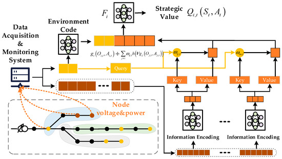
Figure 3.
Network structure of AECN.
The observation–action vector of the distribution substation area agent is encoded into the initial input of the value network, with an initial set of attention weights assigned. The attention network continuously adjusts the attention weight coefficients assigned to each agent during training, enabling the value network to dynamically assess each substation’s contribution to the optimization objective. Based on the adjusted attention weights, the policy network is then guided in making strategy corrections. As shown in Figure 3, for any intelligent agent i, the input to its AECN can be divided into two parts: one part is the environmental information , which represents the agent’s observation-action combination encoding of the distribution network environment, and the other part is the attention information , which encodes the observation–action combinations of the other agents within the cluster:
In the equation, represents the encoding of agent j, where and are the parameters for mapping to the key value and for mapping to the query, respectively. denotes the relevance coefficient that computes the correlation between the observation–action combination of agent i and agent j. is the attention weight coefficient obtained by normalizing , representing the importance of the actions of other agents as observed by agent i in relation to the task at hand.
The Critic network of agent i concatenates the two input parts, resulting in an output , which represents
In the equation, represents a fully connected neural network, is the linear transformation matrix applied to , and h denotes the activation function.
The Critic network update is implemented based on minimizing the joint regression function, with the loss function given by
In the equation, E represents the expectation, and denotes the output of the target Critic network.
The algorithm training process is shown in Algorithm 1. First, the neural network parameters and the experience replay buffer are initialized. Then, the distribution network environment, based on the actions output by the Actor network, performs power flow simulations to compute the node voltage amplitude and active network loss values. The immediate reward is calculated using the reward function in Equation (22). Following this, the system transitions to the next state based on load and substation output. The resulting data from the interaction is stored in the experience replay buffer, completing one interaction cycle. When the data in the experience replay buffer reaches a certain amount, batch data are sampled to train the Critic and Actor networks. The two networks assist each other in training based on the gradient update formulas until convergence. After training is completed, only the Actor network is deployed to the substation. During the online decision phase, control commands are output in real-time through a feedforward pass of the neural network, enabling millisecond-level decision-making for control instructions.
| Algorithm 1 Multi-Agent Reinforcement Learning-Based Coordinated Control Algorithm for Multiple Area Clusters in Distribution Networks |
| →Initialize: the parameters and of the Actor network and Critic of all agents in the area |
| →Initialize: the experience replay buffer, the agents’ learning rates, and the exploration coefficient |
| for epsilon in 1,2,3… do |
| Initialize the distribution network environment |
for t in 1,2,3…T do
|
| end for |
| end for |
5. Algorithm Analysis
5.1. Algorithm System Setup
To validate the effectiveness of the proposed algorithm, simulation experiments were conducted using an improved IEEE 33-bus system with multiple substations. The system’s base capacity is 10 MVA, and the voltage reference value is 12.66 kV. The voltage safety limits were set to 0.95–1.05 p.u. in this study. All buses in the test system are connected to loads, and photovoltaic systems are connected to buses 14, 15, 20, 24, and 32. The locations of the substations 1–9 connected to the distribution network are shown in Figure 4. The daily load and PV active power output during the test day are illustrated in Figure 5.
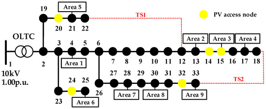
Figure 4.
Topology diagram of modified IEEE33 node system.
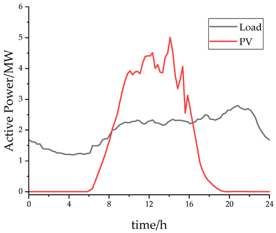
Figure 5.
Load and PV profiles on the test day.
The power flow calculation module for the distribution network is based on the PYPOWER library. The load data used for agent training (including active power from photovoltaic systems) is sourced from actual distribution network data collected over a six-month period. From this dataset, 10 randomly selected days from each month, totaling 60 days, were used as the training set data, while the remaining data were used for testing. The hyperparameter settings for the algorithm are provided in Table 1.

Table 1.
Parameters of the algorithm table.
The cluster partitioning method proposed in Section 1 of this paper was applied to partition the IEEE 33-bus system under different topological structures. The partitioning results are shown in Table 2.
Table 2.
Cluster segmentation results for different topologies.
To evaluate the efficacy of the proposed algorithm, we compare the attention-based action value aggregation approach against two benchmark algorithms:
Comparison Method 1: The action value aggregation method based on the average value, where the attention weight coefficient in Equation (25) is replaced with an average value weight coefficient, as proposed in [20]
Comparison Method 2: The policy transfer learning method, which leverages the transferability of neural networks, and transfers the agent neural network trained in a fixed topology to scenarios with topological changes, as proposed in [21].
5.2. Analysis of the Effects of Regulation
A random day was selected for testing, with the system configured to be in Topology 1 from 00:00 to 10:00, in Topology 2 from 10:00 to 20:00, and in Topology 3 from 20:00 to 24:00. The algorithm is trained for a total of 500 iterations, with validation performed every 10 iterations on the test set to compute the average reward. The reward value curves from 10 experimental runs are shown in Figure 5.
As can be seen from Figure 6, the method proposed in this paper enters the experience accumulation phase during the early stage of training, with the reward values fluctuating significantly. As the training progresses, the agent continuously learns better control strategies from the experience replay pool. After the 50th iteration, the reward gradually increases, and the training converges after 300 iterations.
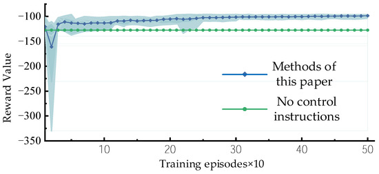
Figure 6.
Reward training curve (Shadow represents the fluctuation range of the reward curves from the results of ten experiments).
Figure 7 illustrates the power output of the three clusters throughout the test day. From Figure 7a, it can be seen that each cluster absorbs reactive power between 08:00 and 16:00, when the PV output is high, and provides reactive power during the remaining hours. Cluster 1, with nodes located at the front end of the distribution network, exhibits lower sensitivity to voltage variations compared to the other two clusters. Therefore, it requires less reactive power support at noon, with a daily average reactive power output of 165.99 kVar. Some nodes in Clusters 2 and 3, located at the feeder ends, are more sensitive to voltage changes and require more reactive power support, with daily average reactive power outputs of 146.71 kVar and 186.75 kVar, respectively. Figure 7b shows that the active power regulation has a smaller impact on the distribution network voltage compared to reactive power regulation. Active power is primarily provided for voltage support during the day (08:00–17:00), with daily average active power outputs of 134.89 kW, 50.85 kW, and 104.7 kW for the three clusters, respectively.
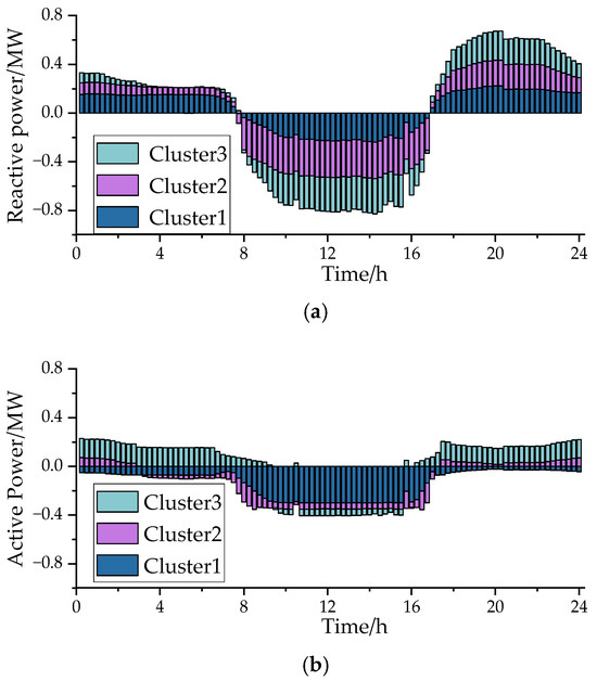
Figure 7.
Cluster power regulation curve. (a) reactive power regulation by cluster; (b) active regulation of clusters.
Figure 8 presents a comparison of node voltages throughout the day using different control methods. The dotted lines correspond to the safe voltage limits. As shown, before the system optimization, the high PV penetration rate caused a significant voltage violation during the periods of high photovoltaic output (10:00–16:00), with the voltage peaking at 1.0841 p.u. at 14:00. From 20:00 to 24:00, due to heavier load, a voltage violation occurred below the lower limit. The overall voltage deviation was large, severely affecting the system’s safe and stable operation. After applying the method proposed in this paper, the voltage level during the noon period was significantly reduced, and the voltage level during the heavy load periods was increased, with overall voltage fluctuations reduced. In comparison with Method 1, the average action value aggregation method raised the overall voltage during 20:00–24:00, but failed to provide sufficient power support from 10:00–16:00, resulting in voltage violations above the safety limit at nodes 14 and 15 with PV integration. Compared to Method 2, although it also regulated the voltage back into the safe range, the overall voltage deviation was not as small as in the proposed method, and Method 2 required additional offline training after the agent in Topology 1 had been trained, leading to slower real-time decision-making compared to the proposed algorithm. In summary, the voltage control effect of the proposed method is superior, as the attention-based action value aggregation method effectively extracts key information that significantly influences the control of the distribution network. It identifies dynamic changes in the clusters of the substation agents caused by topological changes, thus guiding the Actor network to output strategies that adapt to topology variations.
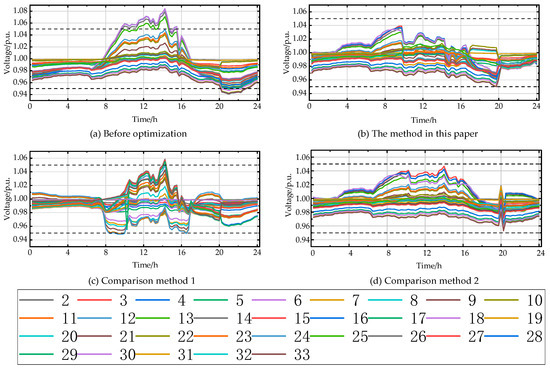
Figure 8.
Voltage distribution of test day nodes under different methods of regulation.
Table 3 presents the voltage indexes and active network loss indexes after applying different control methods. These voltage indexes include the average voltage, maximum voltage, and minimum voltage. As shown in Table 3, the node voltage exceeded the limit severely before regulation, with the maximum voltage reaching 1.0842 p.u. Due to the minimal power flow between nodes under the uncontrolled strategy, the power loss on the transmission lines is relatively low. The proposed method achieves an average voltage closest to the voltage reference value of 1 p.u., and the active network loss only increased by 9.09%, which is less than that of Method 1 and Method 2, indicating better adaptability to topology changes.
Table 3.
Statistics on composite indicators after regulation by different methods.
Since the proposed method in this paper trains each agent offline, the online execution phase requires only the feedforward computation of the neural network, resulting in a runtime of 3.57 milliseconds, which meets the requirements for real-time control.
6. Conclusions
This paper proposes a multi-area collaborative optimization control method for distribution networks, considering topology changes. Based on the Actor–Critic framework, the method models and solves the voltage regulation and loss optimization problem of distribution networks with multiple areas. A Critic network based on the attention mechanism was designed to enhance the scalability of the agent’s observation space in scenarios with topological cluster changes, allowing dynamic adaptation to changes of the cluster boundary. The main conclusions are as follows:
- (1)
- Cluster division of distribution network based on electrical distance modularity index and power balance index can effectively simplify the scale of distribution network optimization problem, reduce the power flow between clusters, and realize distribution network voltage sub-cluster regulation.
- (2)
- The action value aggregation method based on the attention mechanism proposed in this paper can effectively adapt to different topology change scenarios of distribution networks. The simulation results of the improved IEEE33 bus algorithm show that the proposed method significantly reduces voltage deviation and maintains low active network losses, keeping node voltages within the safety range under three topology change scenarios.
Concerning its applicability in distribution networks with a larger number of nodes, future research could apply a transfer-learning-based method. This method could fine-tune the pre-trained intelligent agent network with a small amount of data, thereby enhancing its generalization performance.
Author Contributions
Conceptualization, W.L. and X.M.; Data curation, Y.Z.; Formal analysis, W.L.; Funding acquisition, W.L.; Investigation, X.M.; Methodology, S.Y.; Project administration, S.Y.; Resources, S.Y.; Software, Y.Z.; Supervision, W.L. and X.D.; Validation, Y.Z.; Visualization, Y.Z.; Writing—original draft, W.L.; Writing—review and editing, Y.Z. and X.D. All authors have read and agreed to the published version of the manuscript.
Funding
This research was funded by ‘Research and application of key technologies for distributed photovoltaic intensive control in Huailai rural distribution network, grant number B3018K23000F’.
Data Availability Statement
Data are contained within this article.
Conflicts of Interest
Author Weichen Liang, Xinsheng Ma and Shuxian Yi are employed by the company Electric Power Research Institute, State Grid Jibei Electric Power Co., Ltd. The remaining authors declare that the research was conducted in the absence of any commercial or financial relationships that could be construed as a potential conflict of interest.
References
- Li, P.; Ji, J.; Ji, H.; Jian, J.; Ding, F.; Wu, J.; Wang, C. MPC-Based Local Voltage Control Strategy of DGs in Active Distribution Networks. IEEE Trans. Sustain. Energy 2020, 11, 2911–2921. [Google Scholar] [CrossRef]
- Chen, B.; Chen, C.; Wang, J.; Butler-Purry, K.L. Multi-time step service restoration for advanced distribution systems and microgrids. IEEE Trans. Smart Grid 2017, 9, 6793–6805. [Google Scholar] [CrossRef]
- Lei, S.; Chen, C.; Li, Y.; Hou, Y. Resilient disaster recovery logistics of distribution systems: Co-optimize service restoration with repair crew and mobile power source dispatch. IEEE Trans. Smart Grid 2019, 10, 6187–6202. [Google Scholar] [CrossRef]
- Pesaran, H.M.; Nazari-Heris, M.; Mohammadi-Ivatloo, B.; Seyedi, H. A hybrid genetic particle swarm optimization for distributed generation allocation in power distribution networks. Energy 2020, 209, 118218. [Google Scholar] [CrossRef]
- Cavraro, G.; Arghandeh, R. Multistage robust unit commitment with dynamic uncertainty sets and energy storage. IEEE Trans. Power Syst. 2018, 33, 3500–3509. [Google Scholar] [CrossRef]
- Liu, H.; Wu, W. Two-Stage Deep Reinforcement Learning for Inverter-Based Volt-VAR Control in Active Distribution Networks. IEEE Trans. Smart Grid 2021, 12, 2037–2047. [Google Scholar] [CrossRef]
- Guo, G.; Zhang, M.; Gong, Y.; Xu, Q. Safe multi-agent deep reinforcement learning for real-time decentralized control of inverter based renewable energy resources considering communication delay. Appl. Energy 2023, 349, 121648. [Google Scholar] [CrossRef]
- Su, S.; Zhan, H.; Zhang, L.; Xie, Q.; Si, R.; Dai, Y.; Gao, T.; Wu, L.; Zhang, J.; Shang, L. Volt-VAR Control in Active Distribution Networks Using Multi-Agent Reinforcement Learning. Electronics 2024, 13, 1971. [Google Scholar] [CrossRef]
- Gao, Y.; Wang, W.; Yu, N. Consensus Multi-Agent Reinforcement Learning for Volt-VAR Control in Power Distribution Networks. IEEE Trans. Smart Grid 2021, 12, 3594–3604. [Google Scholar] [CrossRef]
- Sun, W.; He, G. Cluster Partition-Based Voltage Control Combined Day-Ahead Scheduling and Real-Time Control for Distribution Networks. Energies 2023, 16, 4375. [Google Scholar] [CrossRef]
- Fazio, A.R.D.; Risi, C.; Russo, M.; Santis, M.D. Coordinated Optimization for Zone-Based Voltage Control in Distribution Grids. IEEE Trans. Ind. Appl. 2022, 58, 173–184. [Google Scholar] [CrossRef]
- Yan, R.; Xing, Q.; Xu, Y. Multi-Agent Safe Graph Reinforcement Learning for PV Inverters-Based Real-Time Decentralized Volt/Var Control in Zoned Distribution Networks. IEEE Trans. Smart Grid 2024, 15, 299–311. [Google Scholar] [CrossRef]
- Ma, Q.; Deng, C. Simplified Deep Reinforcement Learning Based Volt-var Control of Topologically Variable Power System. J. Mod. Power Syst. Clean. Energy 2023, 11, 1396–1404. [Google Scholar] [CrossRef]
- Jacob, R.A.; Paul, S.; Chowdhury, S.; Gel, Y.R.; Zhang, J. Real-time outage management in active distribution networks using reinforcement learning over graphs. Nat. Commun. 2024, 15, 4766. [Google Scholar] [CrossRef]
- Zhao, Y.; Zhang, G.; Hu, W.; Huang, Q.; Chen, Z.; Blaabjerg, F. Meta-Learning Based Voltage Control for Renewable Energy Integrated Active Distribution Network Against Topology Change. IEEE Trans. Power Syst. 2023, 38, 5937–5940. [Google Scholar] [CrossRef]
- Xiang, Y.; Lu, Y.; Liu, J. Deep reinforcement learning based topology-aware voltage regulation of distribution networks with distributed energy storage. Appl. Energy 2023, 332, 120510. [Google Scholar] [CrossRef]
- Xing, Q.; Chen, Z.; Zhang, T.; Li, X.; Sun, K. Real-time optimal scheduling for active distribution networks: A graph reinforcement learning method. Int. J. Electr. Power Energy Syst. 2023, 145, 108637. [Google Scholar] [CrossRef]
- Newman, M.E.J. Finding community structure in networks using the eigenvectors of matrices. Phys. Rev. E 2006, 74, 036104. [Google Scholar] [CrossRef] [PubMed]
- Li, P.; Zhang, C.; Wu, Z.; Xu, Y.; Hu, M.; Dong, Z. Distributed Adaptive Robust Voltage/VAR Control with Network Partition in Active Distribution Networks. IEEE Trans. Smart Grid 2020, 11, 2245–2256. [Google Scholar] [CrossRef]
- Si, R.; Chen, S.; Zhang, J.; Xu, J.; Zhang, L. A multi-agent reinforcement learning method for distribution system restoration considering dynamic network reconfiguration. Appl. Energy 2024, 372, 123625. [Google Scholar] [CrossRef]
- Ju, Y.; Chen, X. Distributed active and reactive power coordinated optimal scheduling of networked microgrids based on two-layer multi-agent reinforcement learning. Proc. CSEE 2022, 42, 8534–8547. [Google Scholar]
Disclaimer/Publisher’s Note: The statements, opinions and data contained in all publications are solely those of the individual author(s) and contributor(s) and not of MDPI and/or the editor(s). MDPI and/or the editor(s) disclaim responsibility for any injury to people or property resulting from any ideas, methods, instructions or products referred to in the content. |
© 2025 by the authors. Licensee MDPI, Basel, Switzerland. This article is an open access article distributed under the terms and conditions of the Creative Commons Attribution (CC BY) license (https://creativecommons.org/licenses/by/4.0/).