1. Introduction
The world is facing critical challenges in the energy sector, driven by the urgency of climate change and the need to ensure energy security and economic stability [
1]. This scenario is further compounded by the sustained growth in global energy demand, fueled by technological development and population growth, which imposes significant challenges on conventional power systems. Among these challenges are the need to maintain adequate levels of stability and reliability, reduce power losses in transmission and distribution networks, and mitigate the environmental impacts associated with fossil-fuel-based generation.
In this context, the shift towards renewable energy sources, such as solar and wind, has emerged as a fundamental pillar, not only as an alternative to traditional energy sources but also as a key tool to redefine the relationship between the environment, the economy, and social values [
2]. However, this transition also brings inherent challenges, such as the variability and intermittency of these sources, which can compromise the stability and efficiency of power grids. The integration of energy storage technologies (ESSs), particularly battery energy storage systems, has emerged as a strategic solution. These technologies not only enhance the reliability and flexibility of power systems with high renewable penetration but also facilitate a more sustainable energy transition, addressing technical and environmental challenges comprehensively [
3].
ESSs stand out for their versatility and capacity to address issues associated with the intermittency of non-conventional renewable energy sources, such as photovoltaic solar (PV) plants and wind power plants (WPPs), whose generation depends on weather conditions, which are unpredictable. In this context, these systems enable the storage of energy during periods of low demand and high renewable generation availability, allowing it to be released during peak consumption times [
4,
5,
6]. This approach not only enhances the operational efficiency of the electrical system but also contributes to cost reduction by minimizing reliance on fast-response fossil fuel generation units [
7].
In terms of ancillary services, ESSs offer a wide range of functionalities, including frequency regulation [
8,
9,
10,
11], voltage control [
8,
12], and operating reserves. These features are essential for maintaining the quality and continuity of electricity supply, particularly in systems with high penetration of distributed energy resources. Additionally, the ability of ESS to respond almost instantaneously to load and generation fluctuations makes them a strategic tool for ensuring the dynamic stability of the system [
13,
14].
Several researchers have explored battery energy storage systems (ESSs), focusing on optimization, control, and forecasting techniques to enhance performance, economic viability, and integration into energy systems. A reinforcement learning (RL)-based model employing Q-learning with an epsilon-greedy strategy optimizes charging and discharging decisions under uncertain market conditions, ensuring superior economic returns, adaptability, and battery longevity [
15]. Additionally, a risk-preference-based optimization model utilizing Conditional Value-at-Risk (CVaR) evaluates ESS investments, balancing risk and return to tailor strategies based on battery types and economic profiles [
16].
ESS integration into smart grids is exemplified by a Model Predictive Control (MPC) framework that achieves peak shaving under time-varying loads, reducing peak electricity demand and operational costs, emphasizing the financial viability of PV-ESS systems [
17]. A Set-point Frequency Control (SFC) strategy enhances grid stability and reduces balancing costs in high-renewable scenarios, outperforming conventional methods like Maximum Power Point Tracking (MPPT) [
18]. Further innovations include an adaptive multi-functional strategy managing active/reactive power, voltage, and frequency in microgrids, dynamically adjusting power-sharing and state-of-charge (SoC) balancing [
19]. A PI+R control scheme enhances economic dispatch in isolated ESS networks by integrating a reset mechanism, improving convergence speed, stability, and robustness [
20].
Forecasting techniques are pivotal for optimizing ESS performance. A probabilistic model combining Multi-Attention Recurrent Neural Networks (MARNNs), Mixture Density Networks (MDNs), and Monte Carlo Dropout (MCD) accurately predicts state-of-charge (SOC) under Primary Frequency Control (PFC), enhancing decision-making reliability across diverse European regions [
21]. Similarly, a two-level control framework integrates day-ahead and hour-ahead planning for ESS and photovoltaic (PV) systems, employing chance-constrained optimization to manage uncertainties in PV generation and frequency regulation [
22]. Another model for islanded microgrids integrates multi-functional control, enabling ESS participation in ancillary services markets, improving stability, voltage regulation, and load compensation [
23].
Computationally efficient optimization approaches for ESS management in prosumer networks, Renewable Energy Communities (RECs), and microgrids demonstrate economic and scalability benefits. A rule-based scheduling algorithm for low-voltage PV-ESS networks achieves comparable economic gains to linear programming (LP) while reducing computational time by a factor of 30, proving effective for large-scale REC applications [
24].
Techno-economic assessments of ESS integration across residential, industrial, and renewable applications highlight key viability challenges and opportunities. Residential studies emphasize profitability constraints due to ESS costs and electricity pricing, particularly in the Netherlands, with dynamic pricing and net metering (NM) phase-out scenarios [
25]; globally, subsidies or high generation–demand concurrence are necessary for feasibility [
26]. Advanced tools like PVBT incorporate degradation models and optimization to assess ESS economic viability [
27]. Industrial applications explore value stacking, achieving over 136% financial returns compared to single-use cases [
28]. A 500 kW/1065 kWh ESS in Taiwan demonstrates behind-the-meter (BTM) economic feasibility via energy arbitrage and peak shaving, with a discounted payback period of 8.37 years [
29]. ESS also enhances wind farm performance in Thailand, reducing feeder trips and increasing energy output with an internal rate of return (IRR) of 7.74% [
30]. A hybrid system integrating renewable energy, carbon capture, utilization, and storage (CCUS) achieves a 59.78% reduction in carbon emissions with positive net present value (NPV) [
31].
Mixed-integer linear programming (MILP) optimizations refine REC configurations by integrating solar PV and ESS, using two-stage stochastic optimization and unsupervised clustering to address uncertainties in generation and consumption. Peer-to-peer (P2P) energy exchange improves fairness and cost-effectiveness, validated through real-world data [
32].
ESS applications also enhance grid reliability and address technical challenges in transmission and distribution networks. In Brazil, ESS mitigates congestion and supports variable renewable energy (VRE) integration, optimizing power flow across regions; high costs remain a challenge, with “revenue stacking” proposed for economic viability [
33]. A fixed-flexible ESS allocation scheme for wind-integrated networks combines lithium-ion and vanadium redox flow batteries, reducing wind spillage, voltage deviations, and operational costs [
34]. Frequency stability improvements are achieved through an MILP model incorporating transient frequency deviation and rate of change of frequency (RoCoF) constraints, highlighting the need for larger ESS capacities in islanded microgrids due to grid support limitations [
35]. Additionally, a voltage-security-constrained stochastic programming model (VSC-SOBA) optimizes day-ahead ESS scheduling, enhancing voltage stability and grid reliability through active/reactive power capabilities [
36].
Hybrid Energy Storage Systems (HESSs) improve energy reliability in Integrated Energy Systems (IESs) by combining batteries, super-capacitors, flywheels, and hydrogen storage. A comprehensive review of HESS architectures and control methods illustrates their role in enhancing efficiency, lifespan, and power management in microgrids and renewable energy systems [
37].
Table 1 presents a classification of the reviewed literature on ESSs, categorizing citations based on key research areas.
A critical gap in the existing literature is the lack of simultaneous optimization of ESS location, technology selection, and operation while considering the radial nature of distribution networks and associated investment, maintenance, and replacement costs [
38]. To address this, an integrated mathematical formulation is proposed, incorporating these three dimensions within AC microgrids with radial topology. The approach optimizes economic performance and reduces operational costs in high-renewable penetration scenarios. The methodological innovations that can be implemented to achieve these goals include the following:
Master–slave methodology with discrete–continuous coding: A master–slave optimization strategy is proposed where the master stage determines the ESS location, technology selection, and operation under varying generation and demand conditions using a discrete–continuous coding vector; the slave stage is responsible for determining the numerical value of the objective function and ensuring compliance with the set of constraints.
Mathematical model with complex variables: A comprehensive model using complex variables is developed to accurately represent ESS integration and operation. It accounts for investment, maintenance, and replacement costs while incorporating key technical constraints, such as voltage limits, conductor capacities, and ESS charge–discharge cycles.
Performance improvement over existing methods: The proposed methodology outperforms previously reported approaches in both operational cost reduction and computational efficiency. These improvements stem from the use of advanced optimization techniques, including genetic algorithms, particle swarm optimization, and vortex search, along with efficient parallel processing strategies.
In this paper, the master stage is based on the Salp Swarm Optimization Algorithm and focuses on strategic decision making, including the selection of ESS locations, technologies, and daily operation schemes using a discrete–continuous coding vector. On the other hand, the slave stage employs the successive approximations power flow method in its hourly version to evaluate the total annual operating costs of active distribution networks under variable power consumption and renewable energy generation conditions. At the same time, the slave stage ensures compliance with each of the mathematical model constraints through an adaptation function. To accurately model the system, a mathematical formulation based on complex variables is developed, incorporating technical and economic constraints such as investment, maintenance, and replacement costs, voltage limits, and conductor capacities. The following sections detail the mathematical model, the optimization framework, and the computational implementation of the proposed methodology.
The remainder of this document is structured as follows:
Section 2 provides the mathematical formulation, including the objective function and problem constraints.
Section 3 describes the proposed master–slave methodology to address the location, technological selection, and the operation of the ESS.
Section 4 outlines the test feeders and details the test system used to validate the proposed methodology.
Section 5 presents the numerical results, highlighting the main findings from applying the proposed methodology. Finally,
Section 6 discusses the conclusions, limitations, and potential directions for future work.
3. Proposed Methodology
This document presents a master–slave methodology to address the location, technological selection, and operation of ESS in active distribution networks with high penetration of renewable distributed generation. The problem is modeled as a MINLP (
Section 2), where binary variables define the location and technology of the ESS, and continuous variables represent their daily operation. Unlike the methodology presented in [
38], this study employs a discrete–continuous coding vector in the master stage using the Salp Swarm Algorithm (SSA) [
52] to simultaneously determine the locations, technologies, and initial operation schemes of the ESS. The slave stage uses the successive approximation power flow method to evaluate the objective function [
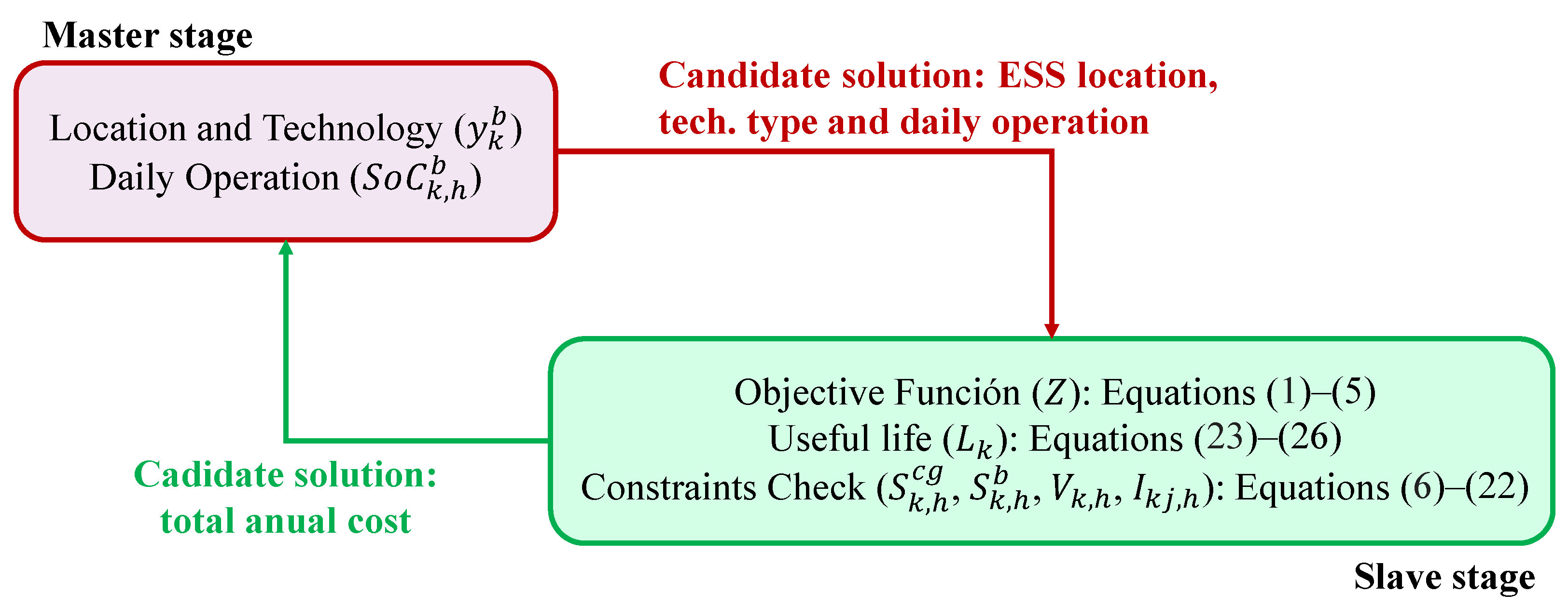
38], which minimizes the total system costs (energy purchase, operation and maintenance, initial investment, and replacement) and verifies compliance with technical and operational constraints. The interaction between both stages is shown in
Figure 1.
Figure 1 illustrates the master–slave approach used in this article, designed to efficiently integrate and operate ESS in active distribution networks. In this framework, the master stage is responsible for high-level decision making, such as determining the location and selecting the technology of battery systems, as well as defining their daily operation scheme. These decisions, represented by variables such as the selected installation nodes and the type of battery used (binary variable
), along with the state of charge (
) of the ESS (continuous variable), form a candidate solution that is subsequently evaluated in the slave stage. This candidate solution is generated by the SSA algorithm.
In the slave stage, the candidate solution is assessed against the network’s technical and economic constraints. This evaluation involves calculating the total annual cost—including energy purchase costs, investment, maintenance, and replacement expenses—and verifying compliance with constraints such as power balance at all nodes, voltage limits, and conductor capacity, among others. To achieve this, key variables are determined, including the power generated at the substation node, , the power absorbed or injected by the ESS, , the voltage at all system nodes, , and the current flowing through each distribution line, . The calculation of these electrical variables is performed using the successive approximations power flow method.
It is important to clarify that the remaining variables in the mathematical model are constant parameters that enable the calculation of the objective function and the evaluation of constraints. This information can be found in
Section 4.
As shown in
Figure 1, each part of the process is linked to specific mathematical expressions, demonstrating how the total cost objective function (
Z) is computed and how the battery lifetime (
) is incorporated into the cost model. Through iterative exchanges between these two stages, the methodology refines the solution, ensuring that the final set of ESS locations, technologies, and operation schemes achieves a balance between technical feasibility and operational cost minimization.
The following sections detail the encoding used to represent the problem, as well as the specific components of each stage of the master–slave methodology.
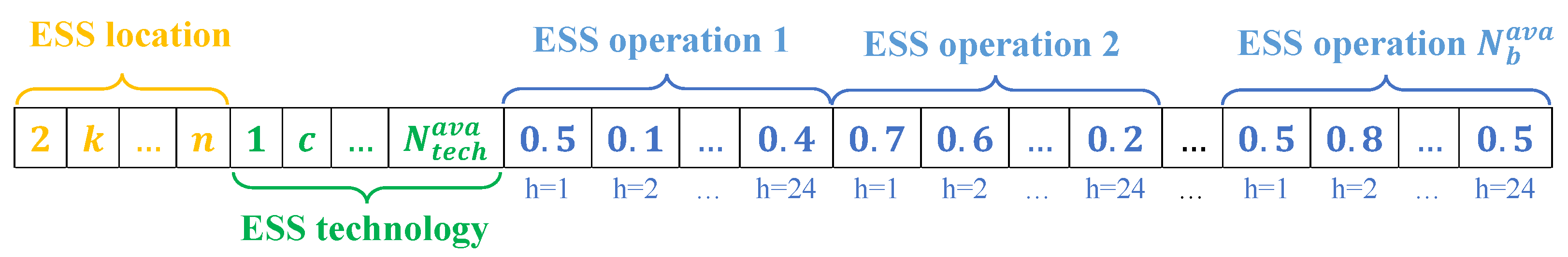
3.1. Proposed Coding
The discrete–continuous coding, illustrated in
Figure 2, efficiently integrates strategic and operational decisions in a single solution, enabling better search space exploration. It ensures effective interaction between discrete (e.g., location, technology) and continuous variables (e.g., daily operation), avoiding inconsistencies and suboptimal solutions common in sequential methods. It avoids the inconsistencies and suboptimal solutions that are typical of sequential methods while enhancing search space exploration, reducing computational time, and ensuring optimization closer to the system’s reality. Furthermore, it minimizes biases between stages and better captures critical interdependencies in complex problems like the planning and operation of electrical systems.
Each candidate solution in
Figure 2 is represented by a vector with two main sections. The first, discrete in nature, is divided into two subsections: the first defines the nodes for ESS installation (yellow), where
k is a random integer between 2 and the total number of system nodes (
n), excluding the generation node as it does not require storage. The second subsection (green) specifies the ESS technology for node
k through a random integer
c, selected from a predefined set of available technological options (
). Notably, the size of the vectors for location and technology selection depends on the number of ESS available for installation (
).
The second section of the vector (blue), continuous in nature, represents the daily operation of the ESS through their SoC over a 24 h horizon (
H). Its size is proportional to the product of the number of installed ESS and the analyzed time periods. Each element corresponds to the SoC of a specific ESS at a given time period (
h); for instance, a value of 0.6 indicates the ESS operates at 60% of its capacity during that period. The discrete–continuous coding used in this study is essential for simultaneously addressing strategic and operational decisions related to the location, technology, and operation of ESS. As demonstrated in prior research [
53], this approach effectively resolves location and sizing problems for photovoltaic units in electrical networks. By integrating the selection of location, technology, and operation into a single vector, the proposed coding enhances search space exploration and reduces processing time, improving the SSA algorithm’s ability to find globally optimal solutions while managing the system’s technical and operational constraints.
3.2. Master Stage: Salp Swarm Algorithm
The SSA is a bio-inspired optimization technique modeled after the coordinated feeding and movement behaviors of salps, gelatinous marine organisms that form chains to enhance their efficiency in searching for food [
52,
54]. These organisms are characterized by their transparent bodies, composed primarily of water and acidic mucopolysaccharides [
55]. SSA, first introduced in recent years, has been widely applied to solve complex combinatorial and continuous optimization problems, demonstrating effectiveness in areas such as the optimal placement and sizing of renewable energy systems [
56,
57,
58,
59].
The step-by-step process used to solve the problem of ESS location, technology selection, and operation in active distribution networks is detailed below. Readers are encouraged to review the original reference for a deeper understanding of the mathematical formulation of the algorithm [
52].
Initialization of the population: The algorithm begins by randomly generating an initial population of candidate solutions, where each solution represents a potential configuration of ESS placement, technology, and operation.Each candidate is encoded as shown in
Figure 2.
Objective function evaluation: Each candidate solution is evaluated using the objective function, which accounts for the total system costs, including energy purchase, ESS integration, maintenance, and replacement costs. The evaluation results are organized with the best-performing solution identified as the leader of the salp chain and the worst solution as the tail of the chain. It is important to note that, once the SSA determines the location, technology, and daily operation of the ESS, this configuration is evaluated using the successive approximation power flow method to calculate the objective function value and ensure compliance with the constraints.
Leader and follower dynamics: The algorithm iteratively updates the positions of the solutions based on leader–follower dynamics. The leader, representing the best current solution, guides the other candidates (followers) through the solution space. This cooperative movement improves the search for optimal configurations by balancing exploration of new areas and refinement of promising regions.
Adaptive movement strategy: To enhance efficiency, the algorithm adjusts its focus between exploration and exploitation as iterations progress. Initially, the algorithm emphasizes exploring the solution space to identify diverse possibilities. Over time, it transitions toward exploitation, refining the most promising solutions for better performance.
Convergence criteria: The iterative process continues until one of two stopping criteria is met; here, the maximum number of iterations is reached, or the solution shows no improvement over a predefined number of consecutive iterations. This prevents unnecessary computation and ensures the algorithm terminates efficiently.
The parameters used in this study are as follows:
- ‑
Maximum number of individuals (salps): 62.
- ‑
Maximum number of iterations: 1000.
- ‑
Maximum number of non-improvement iterations: 250.
In this way, the SSA optimally selects the locations, technologies, and daily operations of the ESS within the active distribution network, achieving the lowest total system costs.
3.3. Slave Stage: Matrix Successive Approximations
The slave stage of the proposed methodology applies a matrix-based successive approximation (MSA) approach, first introduced by [
60], to reduce computation times and iterations needed to evaluate the impact of ESS location, technology, and operation on the system’s annual operational cost. This approach adapts the recursive power flow formula from previous studies [
38], incorporating variations in generation and demand over time.
The successive approximation formula for power flow can be adapted to the context of this study, as follows:
where
represents the voltage at the demand in hour,
h, while
is the inverse of the admittance matrix of the demand nodes, describing their interactions. The term
denotes the element-wise division of the voltage from the previous iteration.
represents the complex power demanded at the network nodes during time period,
h,
corresponds to the power generated by photovoltaic generators, and
is the power injected or absorbed by the ESS in the same period. The matrix
describes the admittance connecting the demand nodes to the substation, and
is the voltage at the substation node during time period,
h, generally assumed to be
for power flow purposes. This iterative process continues until the maximum voltage difference between two consecutive iterations falls below a predefined error threshold.
Once met, the system’s objective function (Equation (
1)) is evaluated. Finally, a penalized fitness function ensures compliance with operational constraints, as shown below. Non-compliant solutions are penalized, adjusting their objective function value. This combined use of matrix-based successive approximations and simultaneous evaluations facilitates rapid and efficient assessment of ESS configurations, enabling the methodology to identify globally optimal solutions while meeting technical and operational constraints.
where
represents the value of the adaptation function, and
is the penalty factor; for this case, it was heuristically selected with a value of
.
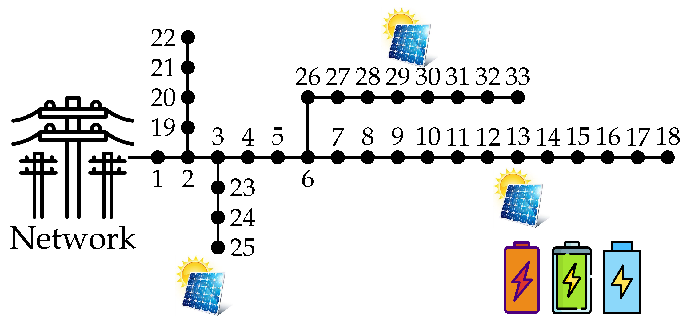
4. Test Feeder
This section details the test system used to validate the proposed methodology. The method was implemented on a widely recognized test system selected from specialized literature (i.e., the 33-node system [
61]). This system has been previously validated and utilized by other authors for similar problems involving ESS integration and operation [
62,
63,
64,
65].
The 33-node test system is characterized by operating at a nominal voltage of 12.66 kV and having an installed capacity of 3715 kW and 2300 kVAr. In this case study, to highlight the advantages and benefits of ESS, three photovoltaic solar generators are included, located at nodes 13 (1125 kW nominal power), 25 (1320 kW nominal power), and 30 (999 kW nominal power), as shown in
Figure 3. It is important to note that the location and size of the renewable generators are based on [
66].
For this case study, three ESS units will be installed in the test system, with the option to select among three different types of ESSs, as shown in
Figure 3. To illustrate this graphically, the available ESS types include: Type A (orange), which has a nominal capacity of 1000 kWh and a charging–discharging time of 4 h; Type B (green), with a nominal capacity of 1500 kWh and a charging–discharging time of 4 h; and Type C (blue), with a nominal capacity of 2000 kWh and a charging–discharging time of 5 h [
38].
The selection of these technologies is based on previous studies reported in the specialized literature, highlighting their advantages in terms of efficiency, charging–discharging time, and nominal capacity—fundamental parameters for optimizing energy storage integration in active networks [
67].
From a technical perspective, the nominal capacity and charging–discharging times of ESS significantly influence their operation. Higher nominal capacities allow for greater energy storage, making them crucial for meeting higher energy demands or sustaining energy supply over longer periods. Conversely, shorter charging and discharging times enable a higher frequency of cycles within the same time frame. These operational characteristics are mathematically represented in Equations (
9), (
14) and (
16). Adjusting the charging–discharging coefficient, along with the maximum and minimum power limits of the batteries, directly affects the SoC and, consequently, the system’s power balance.
The choice of these technologies allows for the analysis of different operational configurations and their impact on system stability and costs, ensuring that the optimization model considers realistic alternatives that are well-documented in the literature.
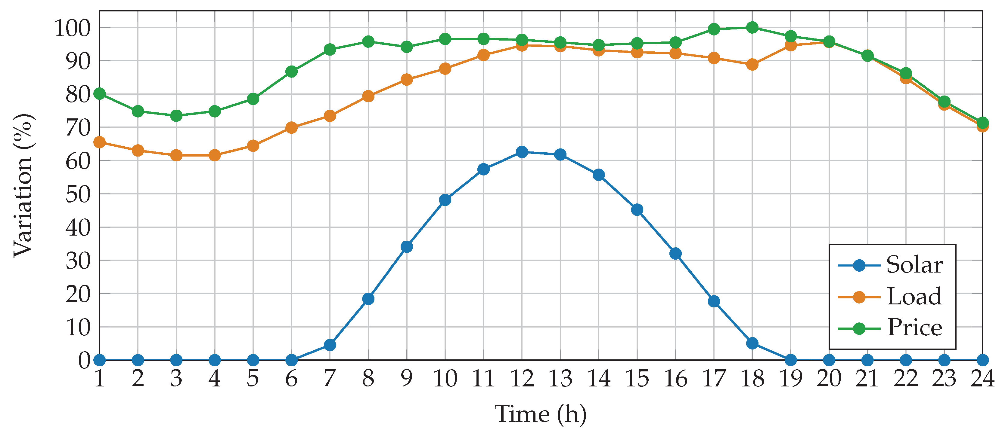
On the other hand, it is important to highlight that this study is contextualized within the climatic and demand conditions of Medellín, the second most populous city in Colombia. The temporal curves used to simulate variations in load, price, and solar generation are shown in
Figure 4 [
38].
Similarly, the information listed in
Table 3 was used to determine the objective function value and ensure compliance with the constraints of the mathematical model [
38].
5. Numerical Results and Discussions
This section presents the main results obtained from applying the proposed methodology. The numerical results were generated using simulations implemented in MATLAB, version R2022a. All simulations were performed on a workstation with a 12th Gen Intel Core i7-12700T CPU @ 1.40 GHz and 32 GB RAM, running on 64-bit Windows 11 Pro. These computational resources provided efficient processing and accurate simulation outputs.
To evaluate the effectiveness of the proposed methodology, it was compared against five approaches that also integrate metaheuristic algorithms. Some of these methodologies have been previously used to address the problem of ESS integration and operation in active distribution networks [
38]. These approaches employ a metaheuristic algorithm in the master stage combined with the vortex search algorithm (VSA) in the slave stage: specifically, the discrete version of particle swarm optimization (DPSO), the discrete Monte Carlo method (DMCM), the discrete version of the Chu–Beasley genetic algorithm (DCBGA), the discrete version of the multi-verse optimizer (DMVO), and the discrete version of the population-based incremental learning approach (DPBIL).
It is worth noting that the previously used algorithms are also based on the master–slave methodology, with the main difference being the use of two metaheuristic algorithms. The first is responsible for solving the location and technology selection problem (discrete encoding), while the second addresses the ESS operation problem (continuous encoding). In contrast, this document implements a single metaheuristic algorithm with a discrete–continuous encoding approach, allowing these two problems to be addressed jointly rather than separately, as has been performed in previous approaches.
5.1. Main Numerical Results
Table 4 shows the numerical values found by applying the proposed approach in the 33-node test system. The table presents the numerical results for the optimization of ESS location, technology selection, and annual cost reduction in a 33-node test system. The baseline case, with no ESS installed, yields an annual cost of USD 2,979,065.61 per year, serving as a reference for evaluating the other methodologies.
The numerical results for each methodology applied to the test system reveal the following:
Each proposed methodology, incorporating ESS installation, achieves cost reductions ranging from USD 12,158.37 per year (DMCM-VSA) to USD 16,605.77 per year (SSA). These results highlight the effectiveness of metaheuristic algorithms in optimizing ESS integration to reduce annual operational costs. However, the SSA methodology achieves the lowest objective function value, indicating its superior performance in identifying optimal ESS configurations for the network.
SSA delivers the highest reduction (USD 16,605.77 per year), followed by DMVO-VSA (USD 14,138.23 per year) and DPBIL-VSA (USD 13,681.24 per year); meanwhile, DMCM-VSA shows the lowest reduction (USD 12,158.37 per year). These differences are primarily due to the appropriate location and technology selection of the various ESS, as well as their operational strategies. The SSA demonstrates superior optimization of decision variables, resulting in the lowest total annual costs. The results emphasize SSA’s effectiveness in reducing annual costs and its potential as the most cost-efficient solution for the test system.
Nodes 2, 5, and 27 are consistently selected across methodologies, underscoring their strategic importance within the network. These nodes experience high power demand as they are either nodes where the system branches or where there is more downstream load, making them ideal for ESS installation to improve stability and reduce total costs. Additionally, their proximity to solar generators at nodes 13, 25, and 30 could play a role, as ESS can help store excess solar generation and balance supply and demand.
Type C ESS (2000 kWh) is predominantly chosen due to its larger capacity and five-hour charging–discharging times, which likely align more effectively with the network’s energy demands and operational requirements. This technology provide greater flexibility in smoothing load profiles, supporting renewable integration, and reducing annual costs.
It is important to note that the difference in objective function values between DMVO-VSA and SSA arises from the operation of the ESS; while both methodologies select the same locations and technologies, SSA’s operational strategy is more efficient, enabling better utilization of the ESS to balance supply and demand. Consequently, SSA achieves a lower annual cost, demonstrating its superior ability to manage the operational aspects of the ESS. In this context,
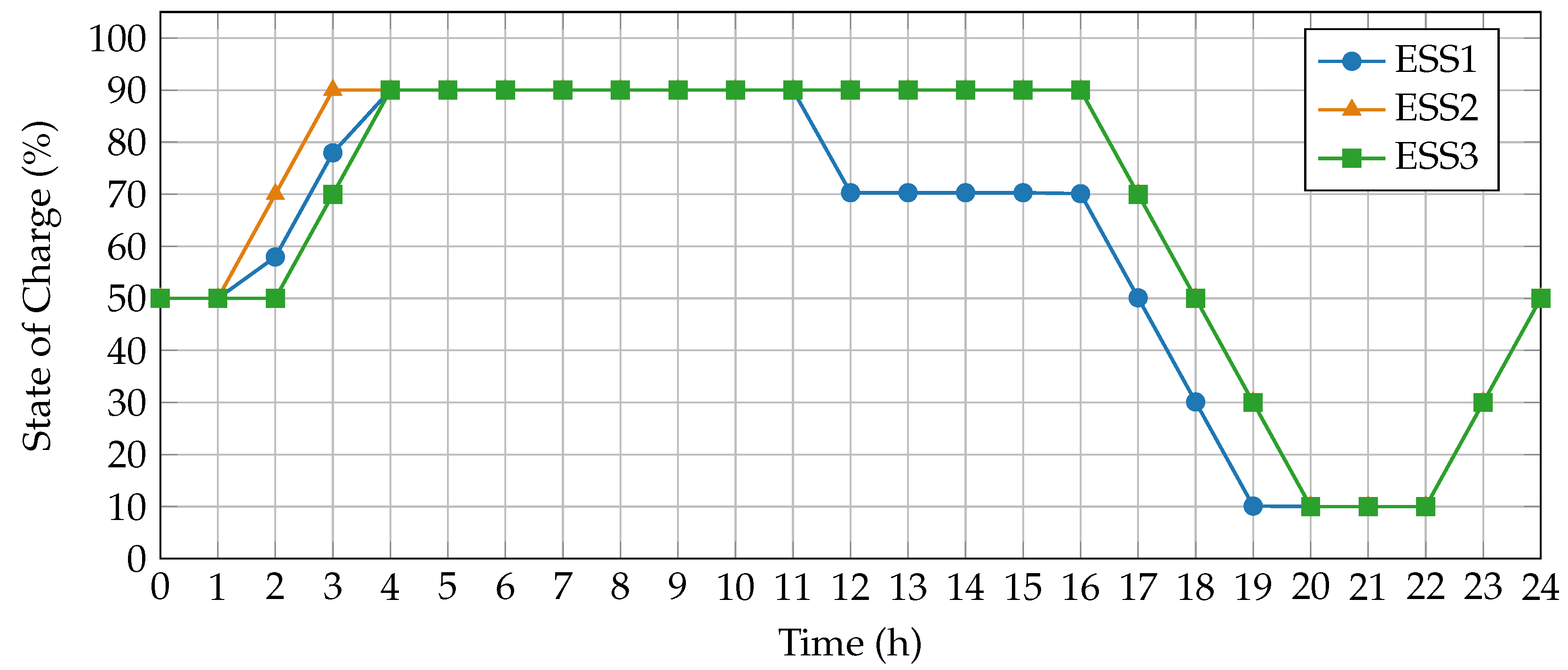
Figure 5 illustrates the operation defined by the SSA for each ESS to minimize the total costs of the test system.
The figure illustrates how each of the three ESSs (ESS1, ESS2, and ESS3) manages active power flows throughout a 24 h period via the SSA methodology. The x-axis represents time in hours (h), while the y-axis shows the state of charge (SoC) as a percentage. Every ESS follows a distinct strategy—ranging from charging to discharging—aimed at optimizing overall system performance by adjusting the active power exchanged with the grid.
In the early hours (0–4), each ESS rapidly charges, bringing SoC above 90%. This charging phase anticipates high-demand periods later in the day while taking advantage of lower energy prices (under 70%). Between hours 4 and 11, the ESS maintain near-full SoC, thus retaining sufficient active power to address upcoming demand peaks. Beginning at hour 6, solar generation supports the network, enabling the ESS to remain charged until higher load conditions arise.
From hour 11 onward, ESS1 begins discharging to meet rising demand, followed by ESS2 and ESS3 from hour 16 as consumption approaches 85% of nominal capacity. With solar production declining after hour 12, the ESSs play a critical role in active power support, gradually releasing stored energy. By hour 19, all three ESS reach minimum SoC, underscoring their importance in balancing supply and demand during peak times. High energy prices (over 90%) further incentivize reduced purchases at the substation node.
In the final hours (21–24), the ESSs recharge in preparation for the subsequent daily cycle, ensuring readiness for the following operational period. Notably, starting around hour 4, ESS2 and ESS3 show almost identical charge–discharge patterns, largely due to their similar technical characteristics and node conditions; consequently, the SSA algorithm converges on analogous operating schedules for both systems. This coordinated active power management ensures each ESS maximizes its availability when needed most, ultimately minimizing total operating costs.
By orchestrating charging and discharging based on demand, solar availability, and pricing, the SSA-based operation scheme guarantees efficient utilization of stored energy. The staggered deployment of active power prevents simultaneous depletion of the ESS units and amplifies the economic benefits for the network. Overall, these results highlight how the proposed methodology leverages active power flows via strategic ESS operation, leading to substantial cost savings and enhanced system performance.
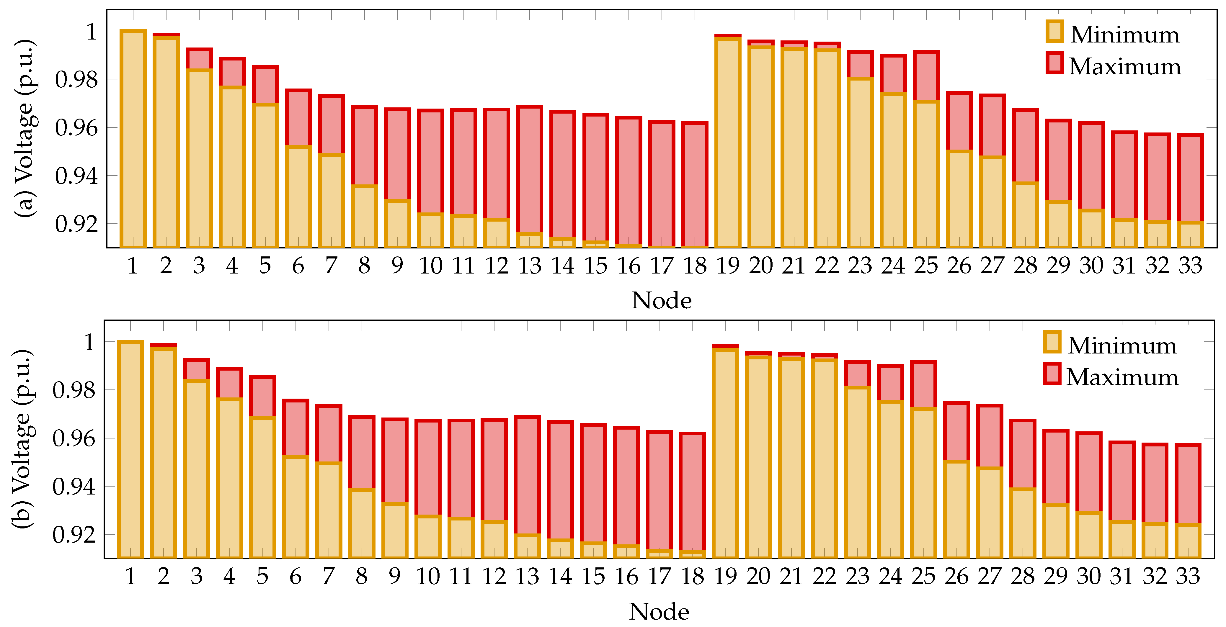
Similarly,
Figure 6 presents the operational state of the 33-node system before and after implementing the solution provided by the SSA approach. This figure illustrates the system’s voltage profiles, showing the minimum and maximum voltage of each node throughout its daily operation.
As shown in
Figure 6, the ESS in active distribution networks can influence voltage profiles. This is evidenced in the graph; here, before ESS integration, the system’s minimum voltage occurs at node 16 with a value of 0.9109 p.u.; whereas, after integration, the minimum voltage is observed at node 18 with a value of 0.91260 p.u. The integration of the ESSs improves the system’s voltage profiles while optimizing its operational costs. It is important to mention that ESS can improve the power factor by supplying reactive power when needed. However, according to constraint (
3) of the mathematical model, ESS do not supply reactive power; therefore, the system’s power factor remains unaffected. Finally, power converters in the ESSs introduce harmonic distortions into the network due to high-frequency switching. The severity of the harmonics depends on the inverter technology and control schemes used. Higher ESS capacities, requiring larger power converters, may exacerbate harmonic content. To mitigate this, active and passive filtering techniques, as well as optimized switching strategies, can be employed.
5.2. Statistical Analysis
To evaluate the performance of the proposed methodology compared to the methodologies used for benchmarking, each algorithm was executed 100 consecutive times to solve the problem of ESS integration and operation in the 33-node test system.
Table 5 presents the numerical results of the optimization methodologies applied to the 33-node test system, summarized in five main columns. The Best Solution (USD) column shows the lowest annual cost achieved by each methodology, while the Average Solution (USD) column provides the mean cost obtained over 100 consecutive evaluations. The Standard Deviation (%) column quantifies the variability of the average results, expressed as a percentage, and the Avg. Time (s) column reports the average computational time required by each methodology to reach a solution.
From
Table 5, we can analyze the following:
The best solution highlights the SSA method as the most effective, achieving the lowest annual cost (USD 2,962,459.8386/year). This demonstrates its superior capability in minimizing system costs. In comparison, the other methodologies yielded higher costs, with differences ranging from USD 2467.54/year (DMVO-VSA) to USD 4447.40/year (DMCM-VSA).
The average solution metric also places SSA as the top performer with the lowest mean cost (USD 2,964,139.9935/year), followed by DMVO-VSA (USD 2,965,728.3329/year) and DPBIL-VSA (USD 2,967,052.4953/year). Methods with higher averages, such as DMC-VSA (USD 2,968,910.9152/year), indicate lower efficiency or consistency in their optimization processes. It is worth noting that the average solution of the SSA surpasses the best solution obtained by the DMVO-VSA (second best), highlighting the consistency and effectiveness of the SSA in delivering high-quality solutions consistently, even across multiple consecutive executions.
In terms of standard deviation, PDMVO-VSA exhibits the highest stability with the lowest variability (0.0200%). The SSA method, while having an intermediate value (0.0416%), still maintains a high level of reliability, as this variability does not significantly impact its overall performance.
The average computational time metric clearly distinguishes SSA as the fastest method, with a time of just 345.71 s. This efficiency is significantly superior to other methodologies, such as PDSSA-VSA (14,596.47 s) and PDPSO-VSA (9632.24 s), which are much slower. PDMVO-VSA (10,214.38 s) represents a balance between computational efficiency and solution quality, but it cannot match SSA’s performance in either aspect.
The analysis confirms SSA as being the most efficient and reliable methodology, excelling in cost minimization and computational time. The established methodologies, while effective, fall short in comparison to SSA’s superior performance. The results also highlight the advantages of using discrete–continuous encoding methods over cascading methodologies that divide the problem into two independent optimization subproblems. This integrated approach enables the simultaneous handling of ESS location and operation, avoiding the limitations inherent in cascading methodologies, where one subproblem is solved first and then the other. In such cases, the initial solution may condition the second step, increasing the risk of the methodology becoming stuck in local optima and limiting the quality of the final results. In contrast, discrete–continuous encoding methods optimize both stages jointly, improving process efficiency and increasing the likelihood of finding global solutions closer to the optimum.
The proposed methodology has been validated on a 33-node test system, yet its underlying mathematical model and metaheuristic implementation are designed to accommodate larger networks. Since the model presented in
Section 2 is independent of specific parametric inputs, it can be adapted to scenarios with more nodes, varied load profiles, and diverse renewable generation portfolios without altering its fundamental structure. However, as the system size increases, computational effort may grow due to the higher dimensionality of the search space. In such cases, parallel processing and efficient initialization strategies can mitigate the increase in computational time. Future work will focus on testing the proposed methodology in distribution systems with over 100 nodes to thoroughly evaluate its scalability and performance under more complex operational conditions.


 ,
, 
