Exact Mixed-Integer Nonlinear Programming Formulation for Conductor Size Selection in Balanced Distribution Networks: Single and Multi-Objective Analyses

Abstract

This paper addresses the optimal conductor selection (OCS) problem in radial distribution networks, aiming to minimize the total costs associated with conductor investment and energy losses while ensuring voltage regulation and power balance as well as observing thermal limits. The problem is formulated as a mixed-integer nonlinear programming (MINLP) model and solved using a hybrid branch-and-bound (B&B), interior-point optimizer (IPO) approach within the Julia-based JuMP framework. Numerical validations on 27-, 33-, and 69-bus test feeders demonstrate cost-efficient conductor configurations. A multi-objective analysis is employed to construct the Pareto front, offering trade-offs between investment and operating costs. The impact of distributed energy resources (DERs) is also assessed, showing cost reductions when said resources provide reactive power support. The results confirm that the proposed MINLP approach outperforms conventional metaheuristics in terms of accuracy and reliability.

1. Introduction

1.1. General Context

Distribution grids play a crucial role in ensuring the reliable and efficient delivery of electrical energy to consumers [1]. As the final link in the power system, these networks connect transmission systems to end-users, facilitating the distribution of electricity at the medium-voltage level [2]. Their proper design and operation are essential for maintaining power quality, minimizing losses, and ensuring system stability [3]. The increasing demand for electricity, the integration of renewable energy sources, and the need for modernization further emphasize the importance of optimizing the performance of distribution networks [4]. Consequently, utilities and regulatory bodies continuously search for strategies to enhance efficiency and sustainability while meeting technical and economic constraints [5].

A key characteristic of electrical distribution networks is their predominantly radial topology, which has become widespread due to its cost-effectiveness and operation simplicity [6]. This structure minimizes investment and operating costs by reducing infrastructure complexity and simplifying protection schemes [7]. However, designing an efficient radial distribution system requires careful consideration of multiple factors, including voltage regulation, power losses, load growth, and reliability [8]. One of the most critical aspects in this context is the optimal selection of conductors, as it directly influences both capital expenditure and long-term operating costs. The conductor sizing problem aims to balance these costs by selecting appropriate conductor gauges that minimize energy losses while maintaining adequate voltage levels and complying with thermal limits [9]. Addressing this problem through advanced optimization techniques can significantly improve distribution network efficiency, ensuring a more sustainable and economically viable power delivery system [10].

1.2. Motivation

Optimal conductor selection (OCS) in electrical distribution networks is a highly complex combinatorial optimization problem [11]. This complexity stems from the discrete nature of the available conductor sizes, the nonlinear electrical relationships governing power flow and energy losses, and the interdependence between investment and operating costs [12]. Additionally, the problem is constrained by thermal limits, voltage drop requirements, and radial topology preservation issues, making traditional heuristic or rule-based approaches insufficient for finding optimal solutions [13]. Conductor selection directly influences both capital expenditure and long-term energy efficiency, requiring a meticulous balance between the minimization of initial investments and the reduction in power losses [10]. Given the large number of possible conductor combinations in medium-voltage distribution networks, exhaustive enumeration is computationally infeasible, highlighting the need for robust optimization methodologies [9].

To address these challenges, an exact optimization approach based on mixed-integer nonlinear programming (MINLP) is essential for rigorously formulating and solving the OCS problem [14]. This work proposes an MINLP-based methodology capable of handling both single and multi-objective analyses to systematically evaluate the tradeoffs between competing economic factors [15]. The two primary objective functions are the costs of investment in conductors and the costs of the expected annual energy losses. These factors significantly impact the financial and operational performance of distribution networks. The single-objective formulation aims to determine the optimal tradeoff between these costs, while the multi-objective analysis aims to construct a Pareto front, offering decision makers a set of optimal solutions with varying levels of investment and energy efficiency. By leveraging an exact optimization framework, this study provides a structured and reproducible approach to the OCS problem, ensuring that distribution networks operate in their most cost-effective and energy-efficient configuration.

1.3. Literature Review

In the scientific literature, multiple approaches have been proposed for solving the OCS problem in radial and balanced distribution networks. Some of these approaches are presented below.

In [14], an MINLP formulation for OCS in radial distribution networks was proposed. The objective was to minimize power losses and conductor investment costs while considering operational constraints such as power balance, voltage regulation, and thermal limits. The model was solved using the GAMS software and the DICOPT solver, conducting numerical tests on 8- and 27-node networks. The results demonstrated the formulation’s effectiveness in selecting conductors under different demand scenarios.

The authors of [13] presented an optimization approach based on Newton’s metaheuristic algorithm (NMA) to solve the OCS problem in three-phase distribution networks. The methodology effectively balanced exploration and exploitation using first- and second-derivative-based evolution rules. According to numerical tests on 8- and 27-node systems, the NMA matched the optimal solution reported in the literature for the smaller system and improved the results in the larger grid. These findings confirm the suitability of the NMA for MINLP problems in electrical distribution networks.

The work by [9] presented a tabu search algorithm (TSA) to optimize conductor selection in electrical distribution networks, with the aim of minimizing investment and operating costs. The algorithm was implemented in the DIgSILENT Power Factory software while considering loadability limits, voltage levels, and operational constraints. Numerical experiments on 27- and 33-node systems demonstrated its effectiveness in balancing investment and operating costs in comparison with existing metaheuristic methods. These findings highlight the algorithm’s potential as a decision support tool for network operators.

In [7], a heuristic approach for the optimal expansion of rural medium-voltage AC distribution grids was proposed. The methodology combined minimum spanning tree-based feeder selection with a TSA to optimize conductor calibers while considering thermal constraints and three-phase power flow simulations in MATLAB 2024b. Numerical tests on 9- and 25-node feeders demonstrated that heuristic initialization provided at least 70% of the calibers in the final solution, enhancing the TSA’s performance. These findings underscore the importance of strategic starting points in metaheuristic optimization for grid planning.

The work presented in [16] described a mixed-integer linear programming (MILP) approach to optimize power distribution systems by integrating OCS and the optimal placement of capacitor banks (OPCB). This combined strategy aimed to minimize technical losses and improve the voltage profile, overcoming the limitations of OCS when used exclusively. As demonstrated by numerical validations on 27-, 69-, and 85-bus test systems, the proposed MILP model outperformed metaheuristic methods reported in the literature. These results highlight the effectiveness of integrating OCS and the OPCB for enhanced distribution system performance.

The authors of [11] presented a discrete version of the vortex search metaheuristic for OCS in three-phase distribution networks. The problem was formulated as an MINLP model, minimizing investment and technical losses costs over a one-year study period. Numerical tests on 8- and 27-node radial systems, as implemented in MATLAB and validated in DIgSILENT, confirmed the method’s effectiveness. Comparative analyses showed that the proposed approach outperformed classical optimization techniques and metaheuristic methods, achieving lower objective function values.

The authors of [17] presented an MINLP model to address the conductor gradation optimization problem in radial distribution systems. Their approach simultaneously optimized conductor size selection and capacitor allocation while incorporating exact AC load flow equations and considering dynamic load characteristics. The primary objective of their model was to ensure compliance with both thermal limits and bus voltage constraints while minimizing capital expenditure on conductors as well as the costs of capacitor installation and energy losses. To validate the proposed nonlinear formulation, a 117-bus radial feeder system was analyzed, demonstrating the effectiveness of the model in optimizing distribution network planning.

The authors of [12] presented the application of the sine–cosine optimization algorithm (SCA) for OCS in radial distribution networks. A conductor library with 20 types based on actual manufacturer data was used to enhance the accuracy of the selection process. The methodology was tested on a real Egyptian distribution system, demonstrating the SCA’s effectiveness in minimizing power losses while observing operational constraints over a ten-year period with high annual load growth. These findings confirmed the suitability of the SCA for long-term network planning.

The study by [10] proposed a multi-criteria decision-making approach based on the CRITIC method to optimize the design of electrical distribution systems. Various design scenarios with different conductor types were evaluated using power flow simulations in Matpower while considering voltage profiles, power losses, current levels, and conductor costs. The methodology was validated on the IEEE 34-bus test system, where a decision matrix of 210 alternatives was analyzed. The results demonstrated the effectiveness of the proposed method in balancing quality, efficiency, and cost in distribution system design.

The reviewed studies collectively address the challenges of OCS and expansion planning in electrical distribution networks through a wide range of optimization techniques, from mixed-integer programming to metaheuristic approaches. A common objective among these works is the minimization of power losses and investment costs while ensuring compliance with operational constraints such as voltage regulation, power balance, and thermal limits. These findings highlight the persistent need for new models and optimization techniques to enhance existing methodologies and further improve solutions to the OCS problem, building upon and surpassing the results reported in the literature.

1.4. Contribution and Scope

Considering the above-presented literature review, this research makes the following key contributions:

• A comprehensive formulation of the OCS problem for radial distribution networks expressed as an MINLP model. This formulation integrates voltage and current variables through the node-to-branch incidence matrix, aiming to minimize both investment and operating costs via single- and multi-objective analyses.
• An efficient solution approach for the proposed MINLP model, leveraging the branch-and-bound method combined with the interior-point approach within Julia’s JuMP optimization framework. This methodology offers significant improvements over the recent literature, which predominantly relies on metaheuristic optimization techniques.

Within the scope of this contribution, the following aspects are considered. First, the studied distribution company has provided the expected demand data for each node, along with the grid topology, which means that the proposed MINLP formulation is exclusively focused on solving the OSC problem. Moreover, the optimization problem is analyzed under peak demand conditions over a one-year study period, as recommended by [9]. Additionally, this research employs a free software tool to demonstrate that, with the appropriate mathematical formulations, large-scale and complex optimization problems in electrical engineering and related sciences can be effectively solved. This is achieved by leveraging powerful solution techniques, specifically the combination of the branch-and-bound method with an interior-point optimizer, which enhances computational efficiency and solution accuracy.

It is important to highlight that, although multiple authors have proposed mixed-integer formulations for addressing the OCS problem in electrical distribution networks [17,18], most of the existing solution methodologies focus on applying master–slave approaches to effectively solve this NP-hard optimization problem [10]. While these methods can be computationally efficient and applicable to large-scale distribution grids, they do not guarantee global optimality or solution repeatability.

In light of these limitations, this research proposes an exact MINLP approach that leverages open-source optimization tools available in the Julia software. By integrating the branch-and-bound (B&B) framework with the interior-point optimization (IPO) method, the proposed methodology ensures high-quality, reproducible solutions [19]. Additionally, this approach facilitates the evaluation of various test system sizes and operational scenarios, including the integration of distributed energy resources (DERs) and other critical factors in distribution network planning.

1.5. Document Structure

The remainder of this document is organized as follows. Section 2 presents the general MINLP formulation of the OSC problem in radial distribution networks with balanced loads, along with an analysis of the model’s nonconvexities and computational complexity. Section 3 details the proposed optimization strategy, which combines the B&B method with an IPO to solve the MINLP formulation. Section 4 describes the main characteristics of the test feeders under study, which consist of 27 and 33 nodes and feature a radial configuration, and it outlines the parametrization of the conductor calibers used in the optimization model. Section 5 presents the numerical validation of the single- and multi-objective models for the test feeders, including a comparative analysis and discussions considering multiple metaheuristic approaches. Finally, Section 6 summarizes the key findings of this study and outlines potential directions for future research.

2. Mathematical Model

OSC for distribution networks is a highly complex optimization problem that integrates graph theory and power flow analysis, resulting in a mixed-integer nonlinear programming (MINLP) formulation [7]. The integer component of this model represents the selection of the conductor types assigned to specific branches, while the continuous one corresponds to the power flow constraints. These constraints, derived from applying Kirchhoff’s laws to the equivalent circuit, result in a system of nonlinear and nonconvex equations. The general formulation of the OSC problem in balanced distribution networks is presented below.

2.1. Objective Functions

OSC is a classical electrical engineering problem that seeks to minimize the expected investment and operating costs of a grid designed to supply electricity to future consumers. The cost components of the objective functions are presented in Equations (1) and (2):

$$\begin{array}{c}\hfill min{z}_1=3C_{\mathrm{kWh}}T\left(\sum _{t\in \mathcal{T}}\sum _{l\in \mathcal{L}}{R}_l{I}_{lt}^2\right),\end{array}$$

(1)

$$\begin{array}{c}\hfill min{z}_1=3\sum _{c\in \mathcal{C}}\left(\sum _{l\in \mathcal{L}}{L}_l{x}_{lc}\right)C_c,\end{array}$$

(2)

where $z_1$ is the objective function that considers the operating costs associated with energy losses; $z_2$ is the objective function representing the conductor investment costs; the parameter $C_c$ denotes the cost coefficient related to the investment made in a conductor of caliber type c; $L_l$ represents the length of branch l; the binary variable $x_{l,c}$ determines the selection of caliber type c for branch l; $C_{\mathrm{kWh}}$ is the average energy cost reported by the utility; T is a time period coefficient; $R_l$ represents the resistance of the conductor assigned to branch l; and $I_{lt}$ is the current magnitude flowing through branch l in period t. Note that $\mathcal{C}$, $\mathcal{L}$, and $\mathcal{T}$ denote the sets corresponding to the conductor sizes, distribution branches, and periods of analysis, respectively.

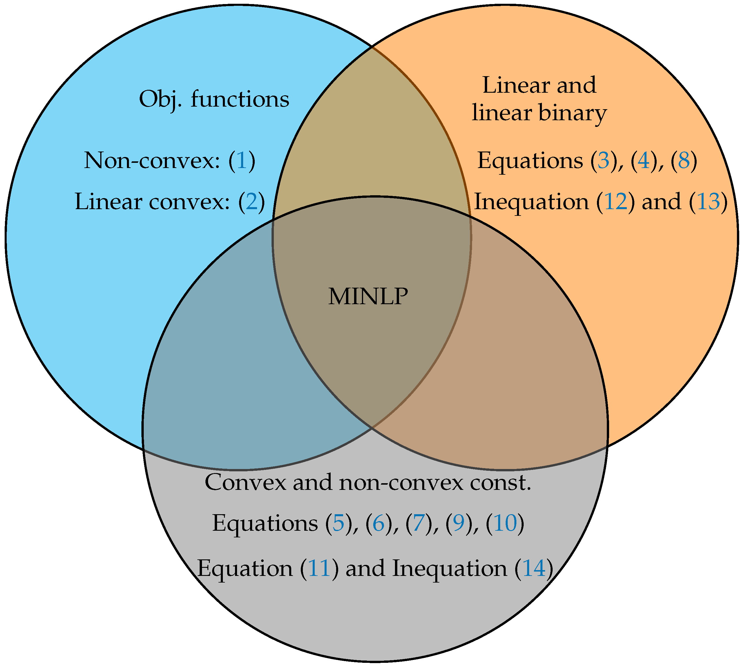
2.2. Set of Constraints

Various technical constraints associated with Kirchhoff’s laws and regulatory policies are considered to ensure the OCS solution’s feasibility. The set of constraints defined from (3) to (14) can be interpreted as follows. Equations (3) and (4) establish the resistance value selected for branch l from the predefined set of available conductor calibers. Equations (5) and (6) describe the real and imaginary components of the current flowing through branch l, which are determined by the voltage difference at the line terminals and by the total branch impedance. Equation (7) defines the current magnitude in branch l as a function of its real and imaginary components.

Constraint (8) ensures that precisely one conductor caliber is assigned to each distribution branch. The active and reactive power balance at bus k during period t is enforced by Inequality Constraints (9) and (10). Equation (11) determines the voltage magnitude at bus k in period t, which is computed based on the real and imaginary components of the voltage. Regulatory policies impose upper and lower limits on this voltage, which are enforced through Box-Type Constraint (12).

Additionally, Inequality Constraint (13) imposes thermal limits on the current flowing through branch l, ensuring that it does not exceed the maximum allowable value for a given conductor caliber c. Finally, Constraint (14) sets the upper bounds for active and reactive power transfer from a generation source connected at bus k in period t, ensuring compliance with operational constraints and system reliability requirements.

The complete Set of Constraints (3) to (14) is mathematically presented below:

$$\begin{array}{cc}\hfill R_l=\sum _{c\in \mathcal{C}}{L}_l{R}_c{x}_{lc},& \left\{\forall l\in \mathcal{L}\right\},\hfill \end{array}$$

(3)

$$\begin{array}{cc}\hfill X_l=\sum _{c\in \mathcal{C}}{L}_l{X}_c{x}_{lc},& \left\{\forall l\in \mathcal{L}\right\},\hfill \end{array}$$

(4)

$$\begin{array}{cc}\hfill I_{lt}^r={\displaystyle \frac{1}{R_l^2+X_l^2}}\sum _{k\in \mathcal{N}}{A}_{kl}\left(R_l{V}_{kt}^r+X_l{V}_{kt}^i\right),& \left\{\forall l\in \mathcal{L},\forall t\in \mathcal{T}\right\},\hfill \end{array}$$

(5)

$$\begin{array}{cc}\hfill I_{lt}^i={\displaystyle \frac{1}{R_l^2+X_l^2}}\sum _{k\in \mathcal{N}}{A}_{kl}\left(R_l{V}_{kt}^i-X_l{V}_{kt}^r\right),& \left\{\forall l\in \mathcal{L},\forall t\in \mathcal{T}\right\},\hfill \end{array}$$

(6)

$$\begin{array}{cc}\hfill I_{lt}=\sqrt{{\left(I_{lt}^r\right)}^2+{\left(I_{lt}^i\right)}^2},& \left\{\forall l\in \mathcal{L},\forall t\in \mathcal{T}\right\},\hfill \end{array}$$

(7)

$$\begin{array}{cc}\hfill \sum _{c\in \mathcal{C}}{x}_{lc}=1,& \left\{\forall l\in \mathcal{L}\right\},\hfill \end{array}$$

(8)

$$\begin{array}{cc}\hfill P_{kt}^g-P_{kt}^d=\sum _{l\in \mathcal{L}}{A}_{kl}\left(I_{lt}^r{V}_{kt}^r+I_{lt}^i{V}_{kt}^i\right),& \left\{\forall k\in \mathcal{N},\forall t\in \mathcal{T}\right\},\hfill \end{array}$$

(9)

$$\begin{array}{cc}\hfill Q_{kt}^g-Q_{kt}^d=-\sum _{l\in \mathcal{L}}{A}_{kl}\left(I_{lt}^i{V}_{kt}^r-I_{lt}^r{V}_{kt}^i\right),& \left\{\forall k\in \mathcal{N},\forall t\in \mathcal{T}\right\},\hfill \end{array}$$

(10)

$$\begin{array}{cc}\hfill V_{kt}=\sqrt{{\left(V_{kt}^r\right)}^2+{\left(V_{kt}^i\right)}^2},& \left\{\forall k\in \mathcal{N},\forall t\in \mathcal{T}\right\},\hfill \end{array}$$

(11)

$$\begin{array}{cc}\hfill V_{min}\le V_{kt}\le V_{max},& \left\{\forall k\in \mathcal{N},\forall t\in \mathcal{T}\right\},\hfill \end{array}$$

(12)

$$\begin{array}{cc}\hfill |I_{lt}|\le \sum _{c\in \mathcal{C}}{I}_c^{max}{x}_{lc},& \left\{\forall l\in \mathcal{L},\forall t\in \mathcal{T}\right\},\hfill \end{array}$$

(13)

$$\begin{array}{cc}\hfill \sqrt{{\left(P_{kt}^g\right)}^2+{\left(Q_{kt}^g\right)}^2}\le S_{kt}^{g,max},& \left\{\forall k\in \mathcal{N},\forall t\in \mathcal{T}\right\},\hfill \end{array}$$

(14)

where $R_c$ and $X_c$ represent the equivalent resistance and reactance values associated with the caliber type c conductor; $I_{lt}^r$ and $I_{lt}^i$ are the real and imaginary components of the current flowing through branch l in period t; $V_{kt}^r$ and $V_{kt}^i$ correspond to the real and imaginary components of the voltage variable related to bus k in period t; $A_{kl}$ defines the component of the admittance matrix relating bus k to branch m; $P_{kt}^g$ and $P_{kt}^d$ are the power generation and demand associated with bus k in period t, respectively, while $Q_{kt}^g$ and $Q_{kt}^d$ represent the same parameters for reactive power; $V_{kt}$ represents the voltage magnitude at bus k in period t, which must be within the minimum and maximum voltage regulation bounds (i.e., $V_{min}$ and $V_{max}$); $I_c^{max}$ corresponds to the maximum current allowed in a caliber type c conductor; and $S_{kt}^{g,max}$ represents the maximum power generation capability associated with the generation source connected to bus k in period t. Note that $\mathcal{N}$ is the set containing all the system nodes.

It should be mentioned that the proposed MINLP formulation is exclusively applicable to balanced distribution networks. This limitation arises because unbalanced scenarios introduce complexities that cannot be captured by a single-phase representation. Specifically, the following are the limitations:

• The presence of unbalanced loads and varying phase impedances hinders the accurate representation of the network using a single-phase equivalent model. Single-, two-, and three-phase loads within the distribution system induce current and voltage imbalances that require a full three-phase formulation.
• A three-phase network may include single- and two-phase laterals, further intensifying voltage and current imbalances. These complexities introduce additional challenges in solving the power flow equations, which are not accounted for in our MINLP approach.

In light of these considerations, our proposed formulation is designed for and limited to balanced distribution grids.

2.3. Mathematical Structure and Complexity

To analyze the mathematical structure and nature of the Optimization Model (1)–(14), the types of equations and inequalities involved must be examined, such as nonlinear, linear, binary, and continuous constraints, along with other relevant characteristics. Figure 1 illustrates the general mathematical structure of the optimization model used to determine the optimal subset of conductor calibers for supplying constant power loads in a radial distribution network.

The main characteristics of the optimization model structure illustrated in Figure 1 are as follows:

• The OCS problem for distribution networks belongs to the family of MINLP problems due to the nonlinear relationships between power, current, and voltage, in addition to the presence of binary variables representing the conductor caliber selected for each branch.
• The primary nonconvexities in the OCS problem arise from power and current balance constraints, voltage and current magnitude calculations, and the objective function related to operating costs, specifically the expected cost of energy losses.
• The Objective Function (1) and the Box-Type Constraint (13) are linear and binary, making them convex for each selected subset of conductor calibers. Meanwhile, the constraints corresponding to the voltage regulation and power transfer capacity at the substation terminals are both convex, with one being linear and the other being conic.

On the other hand, the complexity of the OCS problem defined in (1)–(14) arises from the number of variables, equations, and inequalities present in its MINLP formulation. To assess this issue, let h denote the cardinality of the time periods in the set $\mathcal{T}$, let n represent the number of elements in the set $\mathcal{N}$, let b denote the cardinality of the branches in the set $\mathcal{L}$, and let d correspond to the number of elements in set $\mathcal{C}$. Considering these parameters,

Table 1. Model characterization in terms of the number of variables.

Variable Name	Variable Symbol	Number of Variables
Real current	$I_{lt}^r$	$bh$
Imaginary current	$I_{lt}^i$	$bh$
Current magnitude	$I_{lt}$	$bh$
Real voltage	$V_{kt}^r$	$nh$
Imaginary voltage	$V_{kt}^i$	$nh$
Voltage magnitude	$V_{kt}$	$nh$
Binary	$x_{lc}$	$bd$
Resistance	$R_l$	b
Reactance	$X_l$	b
Active power	$P_{kt}^g$	$nh$
Reactive power	$Q_{kt}^g$	$nh$
Total variables		$\left(3b+5n\right)h+\left(d+2\right)b$

defines the number of variables in the OCS problem.

Considering the information on the formulation’s number of variables (Table 1), for a test feeder composed of 33 nodes, 32 branches, 24 periods of study, and eight caliber types, the number of variables to be established during the optimization process is 6584. In addition,

Table 2. Model characterization in terms of the number of equations, inequalities, and objective functions.

Equation Name	Equation Number	Number Constraints
Operating costs	(1)	1
Investment costs	(2)	1
Resistance	(3)	b
Reactance	(4)	b
Real current	(5)	$bh$
Imaginary current	(6)	$bh$
Current magnitude	(7)	$bh$
Caliber selection	(8)	b
Real voltage	(9)	$nh$
Imaginary voltage	(10)	$nh$
Voltage magnitude	(11)	$nh$
Voltage regulation	(12)	$nh$
Thermal limitation	(13)	$bh$
Power generation	(14)	$nh$
Total equations and inequalities		$\left(4b+5n\right)h+2\left(1+b\right)$

lists the number of equality and inequality constraints and objective functions associated with the OCS problem. Note that, with the same inputs for calculating all the variables, the number of equalities and inequalities is 7098.

Finally, regarding the dimension of the solution space, it is important to mention that there are billions of possible combinations of the binary variables, and each of them generates a reduced nonlinear programming model. To solve the OCS problem, the number of potential solutions for all the binary variables takes the following structure:

$$\begin{array}{c}\hfill \dim =d^b,\end{array}$$

(15)

which is clearly an exponential dimension in the case of the aforementioned example, i.e., $b=32$, and $c=8$. Thus, the dimension of the solution space is larger than $7.9228163\times {10}^{28}$.

3. Solution Methodology

This study employs a solution approach that combines the B&B algorithm with an IPO to effectively solve the MINLP problem at hand [20]. The methodology exploits the capabilities of the B&B method to manage integer variables while utilizing IPO to solve the nonlinear programming (NLP) subproblems that emerge during the branching process [21].

3.1. Overview of the B&B Algorithm

The B&B algorithm is a global optimization technique commonly used to solve MINLP problems by systematically exploring and partitioning the solution space while pruning suboptimal branches through bounding mechanisms [22]. The key steps of the B&B method applied in this study are presented below.

The B&B algorithm follows a structured process to efficiently solve MINLP problems. Initially, the integer constraints are relaxed, converting the problem into a continuous NLP formulation. The relaxed problem is then solved using an IPO, which effectively handles nonlinear constraints and large-scale optimization problems. If the obtained solution does not satisfy integer feasibility, the algorithm proceeds to the branching phase, where the problem is divided into multiple subproblems by fixing one or more integer variables. As the search tree expands, bounding mechanisms are applied by updating the lower and upper bounds of each node, allowing for the pruning of suboptimal or infeasible branches. This iterative process continues until an integer-feasible solution is found which satisfies optimality criteria or until the bounding gap falls within a predefined tolerance, ensuring convergence to the global optimum.

3.2. Interior-Point Optimizer

At each node of the B&B tree, the IPO method is employed to efficiently solve the corresponding continuous NLP subproblems [23]. This method is particularly well suited for large-scale optimization due to its polynomial-time complexity and its ability to effectively manage nonlinear constraints. Within the B&B framework, IPO plays a crucial role in improving computational efficiency by providing strong lower bounds that enhance the pruning process [24]. Additionally, it ensures numerical stability while solving NLP relaxations and facilitates the convergence of highly constrained MINLP problems. These advantages make IPO a powerful tool for handling complex optimization tasks within the B&B approach.

3.3. Implementation Framework

The proposed methodology was implemented using an optimization modeling framework that supports both B&B and IPO solvers (i.e., the Julia software with its JuMP optimization environment [25]). The implementation consists of the following key components:

• Problem formulation: The MINLP problem is structured with a set of nonlinear constraints, integer decision variables, and a nonlinear objective function, ensuring a comprehensive representation of the optimization problem.
• Solver selection: A hybrid solver capable of integrating the B&B method with IPO was selected to efficiently handle the optimization process, i.e., Juniper with the HiGHS and Ipopt optimizers of the Julia software 1.9.2 [25].
• Computational procedure: The model is iteratively solved at each node of the B&B tree, where the IPO solver is used for NLP relaxation. Branching and bounding mechanisms are systematically applied until the convergence criteria are met, thereby ensuring an optimal solution.

Note that Julia software offers a powerful and flexible environment for tackling complex optimization problems, making it an invaluable tool for both researchers and industry professionals [25]. Its high-performance computing capabilities, seamless integration with advanced solvers, and user-friendly syntax enable efficient modeling and solving of large-scale nonlinear and mixed-integer optimization problems [26]. By leveraging Julia’s speed and extensive optimization libraries, industries can enhance decision-making processes, while researchers can develop and test cutting-edge algorithms with minimal computational overhead.

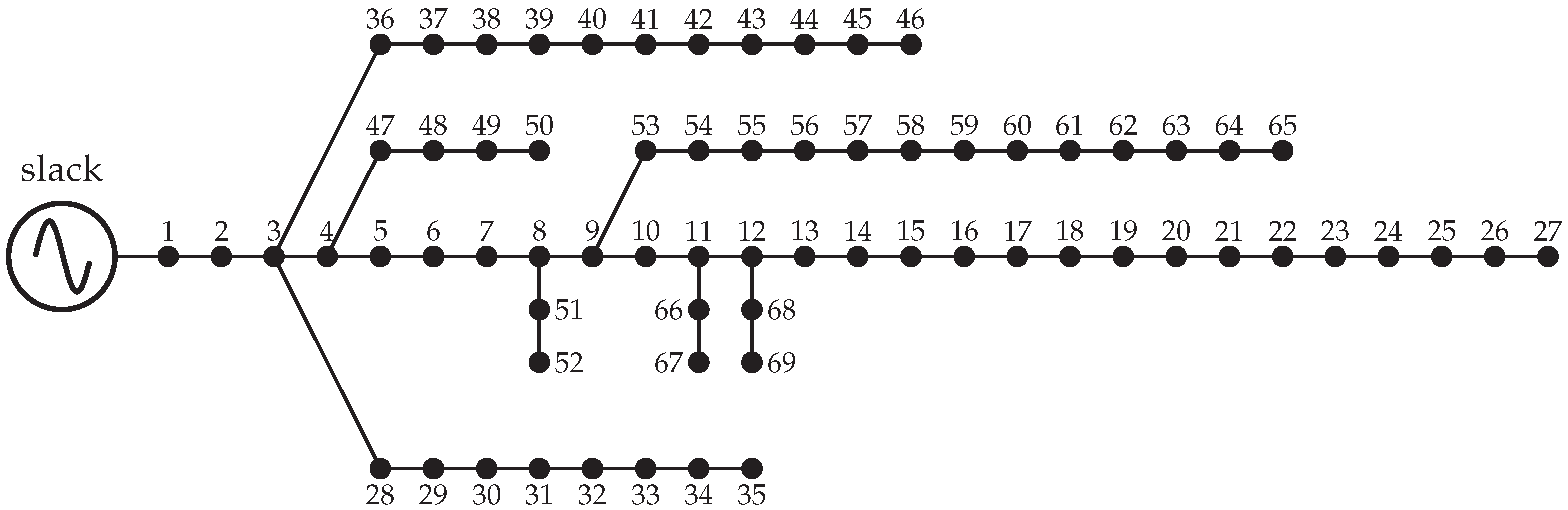
4. Test Feeder Characterization

To assess the effectiveness of the proposed solution methodology, two benchmark test systems commonly referenced in the specialized literature were employed [9]. These systems consist of 27 and 33 nodes, featuring a radial configuration and operating under balanced conditions. In both distribution feeders, all loads were modeled with star connections, which can lead to higher power losses. The main characteristics of each system are detailed below.

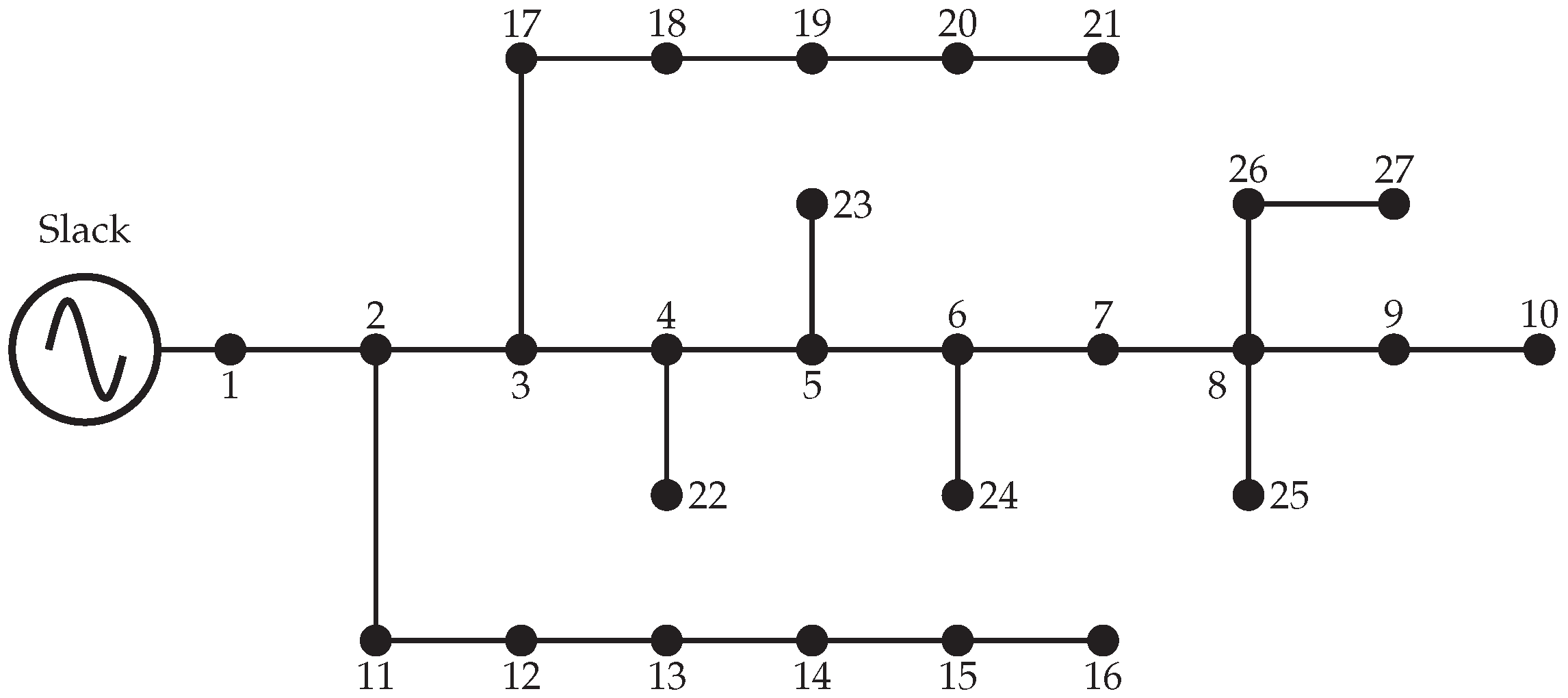
4.1. 27-Bus System

The 27-node test system is a three-phase radial distribution network operating at a phase-to-neutral voltage of 13.8 kV, with a unitary power factor at the substation node (Figure 2) [9].

Table 3. Electrical parameters of the 27-bus grid.

Line l	Node k	Node m	${\mathit{L}}_{\mathit{l}}$ (km)	${\mathit{P}}_{\mathit{mt}}^{\mathit{d}}$ (kW)	${\mathit{Q}}_{\mathit{mt}}^{\mathit{d}}$ (kvar)	Line l	Node k	Node m	${\mathit{L}}_{\mathit{l}}$ (km)	${\mathit{P}}_{\mathit{mt}}^{\mathit{d}}$ (kW)	${\mathit{Q}}_{\mathit{mt}}^{\mathit{d}}$ (kvar)
1	1	2	0.55	0	0	14	14	15	1.00	106.3	65.8
2	2	3	1.50	0	0	15	15	16	1.00	255	158
3	3	4	0.45	297.5	184.4	16	3	17	1.00	255	158
4	4	5	0.63	0	0	17	17	18	0.60	127.5	79
5	5	6	0.70	255	158	18	18	19	0.90	297.5	184.4
6	6	7	0.55	0	0	19	19	20	0.95	340	210.7
7	7	8	1.00	212.5	131.7	20	20	21	1.00	85	52.7
8	8	9	1.25	0	0	21	4	22	1.00	106.3	65.8
9	9	10	1.00	266.1	164.9	22	5	23	1.00	55.3	34.2
10	2	11	1.00	85	52.7	23	6	24	0.40	69.7	43.2
11	11	12	1.23	340	210.7	24	8	25	0.60	255	158
12	12	13	0.75	297.5	184.4	25	8	26	0.60	63.8	39.5
13	13	14	0.56	191.3	118.5	26	26	27	0.80	170	105.4

provides system data corresponding to balanced operating conditions, with the load information specified on a per-phase basis.

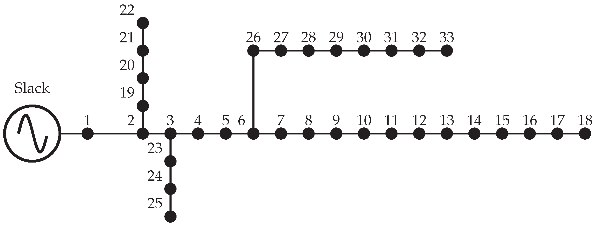
4.2. 33-Bus System

The second test feeder is a 33-node three-phase distribution network with a radial configuration. It operates at a phase-to-neutral voltage of 12.66 kV and maintains nominal voltage at the substation node (Figure 3) [9].

Table 4. Electrical parameters of the 33-bus grid.

Line l	Node k	Node m	${\mathit{L}}_{\mathit{l}}$ (km)	${\mathit{P}}_{\mathit{mt}}^{\mathit{d}}$ (kW)	${\mathit{Q}}_{\mathit{mt}}^{\mathit{d}}$ (kvar)	Line l	Node k	Node m	${\mathit{L}}_{\mathit{l}}$ (km)	${\mathit{P}}_{\mathit{mt}}^{\mathit{d}}$ (kW)	${\mathit{Q}}_{\mathit{mt}}^{\mathit{d}}$ (kvar)
1	1	2	0.0699	100	60	17	17	18	0.6530	90	40
2	2	3	0.3720	90	40	18	2	19	0.1603	90	40
3	3	4	0.2762	120	80	19	19	20	1.4298	90	40
4	4	5	0.2876	60	30	20	20	21	0.4439	90	40
5	5	6	0.7630	60	20	21	21	22	0.8231	90	40
6	6	7	0.4030	200	100	22	3	23	0.3798	90	40
7	7	8	1.4733	200	100	23	23	24	0.8035	420	200
8	8	9	0.8850	60	20	24	24	25	0.7985	420	200
9	9	10	0.8900	60	20	25	6	26	0.1532	60	25
10	10	11	0.1308	45	30	26	26	27	0.2145	60	25
11	11	12	0.2491	60	35	27	27	28	0.9963	60	20
12	12	13	1.3115	60	35	28	28	29	0.7524	120	70
13	13	14	0.6272	120	80	29	29	30	0.3830	200	600
14	14	15	0.5585	60	10	30	30	31	0.9687	150	70
15	15	16	0.6457	60	20	31	31	32	0.3362	210	100
16	16	17	1.5050	60	20	32	32	33	0.4356	60	40

summarizes the system data under balanced operating conditions, with the load details specified on a per-phase basis.

4.3. Type of Conductors Available

To assess our proposal’s effectiveness, eight conductor types applicable to both test systems were analyzed [9]. The characteristics of these conductors are detailed in

Table 5. Conductor types available for installation in the 27- and 33-bus grids.

Caliber c	${\mathit{R}}_{\mathit{c}}$ ($\mathbf{\Omega }$/km)	${\mathit{X}}_{\mathit{c}}$ ($\mathbf{\Omega }$/km)	${\mathit{I}}_{\mathit{c}}^{max}$ (A)	${\mathit{C}}_{\mathit{c}}$ (USD/km)
1	0.8763	0.4133	180	1986
2	0.6960	0.4133	200	2790
3	0.5518	0.4077	230	3815
4	0.4387	0.3983	270	5090
5	0.3480	0.3899	300	8067
6	0.2765	0.3610	340	12,673
7	0.0966	0.1201	600	23,419
8	0.0853	0.0950	720	30,070

, which includes the average positive-sequence impedance per kilometer of network along with the associated cost. Note that the investment cost per kilometer of conductors shown in Table 5 is given per phase. Therefore, in the objective function defined in (2), the investment costs are multiplied by three to account for their application in three-phase networks.

Note that the investment costs reported for the conductors inherently include the associated supporting structures, such as poles, insulators, and crossarms. Given that the choice of conductor type directly affects structural requirements, these elements have been incorporated into the total investment calculations.

5. Numerical Results

The computational implementation of our proposal was carried out using the Julia software, version $\mathrm{1.9.2}$ [27], on a PC equipped with an AMD Ryzen 7 3700 processor (2.3 GHz) and 16.0 GB RAM, running a 64-bit version of Microsoft Windows 10 Single Language. The proposed MINLP model was solved within the JuMP optimization framework, utilizing the Ipopt and HiGHS solvers via the Juniper optimizer [25,28].

All numerical validations focused on solving the OCS problem using both single- and multi-objective frameworks. In the single-objective case, the optimization aimed to minimize the total investment and operating costs (in the 27-, 33-, and 69-bus grids under study). Meanwhile, the multi-objective approach employed a weighting-based optimization strategy to construct the optimal Pareto front. The following sections provide a detailed analysis and discussion of both approaches using the 27- and 33-bus grids as test feeders.

Note that the expected costs of energy losses per kilowatt (i.e., $C_{\mathrm{kWh}}$) were set at USD/kWh 0.1390, as per the recommendations of [9].

5.1. Single-Objective Analysis

To evaluate the classical approach to solving the OCS problem, a single-objective analysis was conducted. Following this approach, both objective functions were linearly combined, leading to the formulation of the following equivalent optimization problem:

$$\begin{array}{cc}\hfill \mathrm{Objective}\mathrm{function}:& min{z}_3=z_1+z_2,\hfill \end{array}$$

(16)

Subject to: (3)–(14).

This objective function aims to balance investment and operating costs to achieve the most cost-effective solution for distribution system planning from the perspective of the distribution company.

5.1.1. Results for the 27-Bus Grid

Table 6. Results comparison for the 27-bus grid.

Method	Gauges	Investment (USD)	Losses (USD)	Annual Cost (USD)
VSA	$\left[\begin{array}{c}7,7,5,4,4,3,3,1,1,\\ 4,4,2,3,2,1,4,4,2,\\ 2,2,1,1,2,2,1,1\end{array}\right]$	344,352.1500	217,066.2509	561,418.4009
NMA	$\left[\begin{array}{c}7,7,4,4,4,4,3,1,1,\\ 4,4,3,3,1,2,4,3,2,\\ 1,1,1,1,2,2,1,1\end{array}\right]$	337,744.8000	219,343.8588	557,088.6588
GNDO	$\left[\begin{array}{c}7,7,4,4,4,3,3,1,1,\\ 4,4,2,1,1,1,3,2,2,\\ 1,1,1,1,1,1,1,1\end{array}\right]$	319,768.0800	230,953.1781	550,721.2581
TSA	$\left[\begin{array}{c}7,7,4,4,4,3,3,1,1,\\ 4,4,2,1,1,1,4,2,2,\\ 1,1,1,1,1,1,1,1\end{array}\right]$	323,593.0800	227,087.1727	550,680.2527
MINLP	$\left[\begin{array}{c}7,7,4,4,4,3,3,1,1,\\ 4,4,2,1,1,1,4,2,2,\\ 1,1,1,1,1,1,1,1\end{array}\right]$	323,593.0800	227,087.1727	550,680.2527

provides a comparative evaluation of different optimization methodologies for conductor selection in the 27-bus radial distribution system. The performance of the proposed MINLP formulation, implemented in Julia’s JuMP environment, was analyzed against four metaheuristic-based approaches: the vortex search algorithm (VSA), the Newton metaheuristic algorithm (NMA), the generalized normal distribution optimizer (GNDO), and the TSA, as reported in [9].

Considering the results shown in Table 6, the following observations can be made:

• The investment cost represents the initial expenditure required for implementing the selected conductor configuration. Among the metaheuristic methods, the GNDO achieved the lowest investment cost at USD 319,768.08, while the VSA reported the highest value: USD 344,352.15. The MINLP formulation, along with the TSA, resulted in an investment cost of USD 323,593.08, which is lower than the VSA and the NMA but slightly higher than the GNDO. This suggests that, while heuristic approaches can reduce initial expenditure, they may not necessarily lead to optimal long-term solutions.
• The cost associated with power losses significantly impacts the long-term economic feasibility of the selected configuration. The VSA reported the lowest power losses cost (USD 217,066.25), whereas GNDO had the highest value (USD 230,953.18). The MINLP and TSA formulations both exhibited a losses cost of USD 227,087.17, which is lower than the GNDO but slightly higher than the NMA (USD 219,343.86). These differences indicate that some algorithms prioritize lower initial investments at the expense of higher operational losses, affecting the overall economic performance of the system.
• The total annual cost, which combines investment and power losses, serves as a key metric for assessing the overall system efficiency. The MINLP approach, along with the TSA, achieved the lowest annual cost (USD 550,680.25), which makes them the most cost-effective solutions. In contrast, the VSA reported the highest total cost (USD 561,418.40), mainly due to its elevated investment costs. The GNDO, despite yielding the lowest investment cost, incurred higher power losses, leading to an annual cost of USD 550,721.26, being slightly above that of the MINLP formulation and the TSA. This confirms that optimizing for investment alone does not necessarily lead to the most cost-efficient solution over time.
• The conductor gauge selection of each approach clearly reflects its nature. The solutions obtained with the TSA and the MINLP formulation are identical, indicating that the latter successfully converged to a globally optimal or near-optimal solution. The differences in conductor configurations across the other methodologies likely contributed to variations in both investment and power losses costs. The ability of MINLP to achieve the same results as the TSA further supports its reliability in finding high-quality solutions without relying on stochastic search processes.
• The fact that the MINLP formulation and the TSA reached the same total cost and conductor configuration suggests that the former provides a structured and deterministic alternative to metaheuristic techniques. Unlike heuristic methods, which depend on parameter tuning and randomness, MINLP guarantees a mathematically structured optimization process, leading to more predictable and repeatable outcomes. The observed variations in investment and power losses costs across the different metaheuristic approaches highlight their sensitivity to the search strategies and parameter settings used, whereas MINLP ensures solution reliability through systematic constraint handling and objective function optimization.

This comparative analysis highlights that the proposed MINLP formulation effectively balances investment and losses costs, achieving the lowest total annual cost alongside the TSA. While some metaheuristic approaches such as the GNDO reduce the initial investment costs, they result in higher power losses, leading to increased operational expenses over time. On the other hand, the VSA minimizes the losses costs but requires significantly higher initial investments. The results demonstrate that the MINLP formulation provides a structured and competitive alternative to heuristic approaches, offering an optimal balance between capital investment and long-term operational efficiency.

5.1.2. Results for the 33-Bus Grid

Table 7. Results comparison for the 33-bus grid.

Method	Gauges	Investment (USD)	Losses (USD)	Annual Cost (USD)
TSA	$\left[\begin{array}{c}7,7,5,5,5,4,3,2,1,\\ 1,1,1,1,1,1,1,1,1,\\ 1,1,1,3,2,1,4,4,4,\\ 3,3,1,1,1\end{array}\right]$	209,773.4628	215,137.5583	424,911.0211
MINLP	$\left[\begin{array}{c}7,7,7,5,5,4,3,2,1,\\ 1,1,1,1,1,1,1,1,1,\\ 1,1,1,3,2,1,4,4,4,\\ 3,3,1,1,1\end{array}\right]$	222,494.1300	201,987.5249	424,481.6549

provides a comparative evaluation of the results obtained regarding conductor selection in the 33-bus feeder. The performance of the proposed MINLP formulation was analyzed against the TSA approach reported by [9].

The numerical results presented in Table 7 provide valuable insights into the performance of the MINLP and TSA approaches for optimizing conductor selection in the 33-bus system. The following key observations can be made:

• The comparison reveals that both the MINLP formulation and the TSA yielded similar solutions in terms of conductor gauge selection, investment cost, energy losses cost, and total annual cost. However, a distinct trade-off was observed between the initial investment and the operational losses, highlighting the contrasting optimization strategies of the two approaches.
• The conductor investment cost obtained using the MINLP method amounted to USD 222,494.13, which is USD 7356.57 (3.42%) higher than that required by the TSA (USD 215,137.56). On the other hand, the energy losses cost of the MINLP formulation came out to USD 201,987.52, which is USD 7785.94 (3.71%) lower than that obtained with the TSA (USD 209,773.46). This indicates that MINLP prioritizes long-term operational efficiency by reducing energy losses, whereas TSA focuses on minimizing the initial investment costs.
• The increased investment cost of the MINLP solution suggests that its optimization strategy emphasizes reducing resistive losses over the system’s lifetime, leading to improved long-term economic performance. In contrast, the TSA seeks to minimize upfront expenses, potentially resulting in slightly higher operating costs due to greater energy losses over time.
• Despite these differences, the total annual cost of the TSA and the MINLP method remains nearly identical. The TSA solution led to an annual cost of USD 424,911.02, while the MINLP approach yielded USD 424,481.65. The absolute difference of USD 429.37 (0.1%) confirms that both methods achieve a comparable cost efficiency, implying that the choice between them depends primarily on whether the priority is minimizing the initial investment (TSA) or reducing long-term losses (MINLP).

This comparative analysis highlights that both MINLP and the TSA can effectively optimize conductor selection in the 33-bus system, leading to an efficient network configuration. However, the MINLP formulation provides a more structured and mathematically rigorous approach, ensuring global optimality and repeatability in the decision-making process. These findings underscore the relevance of integrating exact optimization techniques alongside metaheuristic methods to enhance the robustness and efficiency of power distribution system planning.

5.2. Multi-Objective Analysis

Multi-objective analysis is an alternative optimization approach that seeks to evaluate the compromise between different conflicting objective functions. This work adopted the weighting-based optimization approach to construct the optimal Pareto front [29]. The resulting optimization model is presented below:

$$\begin{array}{cc}\hfill \mathrm{Objective}\mathrm{function}:& min{z}_3=\omega z_1+\left(1-\omega \right)z_2,\hfill \end{array}$$

(17)

Subject to: (3)–(14).

$$\begin{array}{c}\hfill {\omega }_{min}\le \omega \le {\omega }_{max}\end{array}$$

(18)

where $\omega$ is the weighting factor that determines the relative importance of each objective. In this optimization approach, $\omega$ is varied using a predefined step size. Note that ${\omega }_{min}$ and ${\omega }_{max}$ are the maximum values allowed for the weighting factors $\omega$, which were set between 20% and 80% in this research.

5.2.1. The 27-Bus Grid

Table 8. Pareto front for the 27-bus system.

$\mathit{\omega }$	${\mathit{z}}_1$ (USD)	${\mathit{z}}_2$ (USD)	${\mathit{z}}_1+{\mathit{z}}_2$ (USD)
0.20	457,519.2268	184,516.2768	642,035.5036
0.25	433,692.1077	191,583.4391	625,275.5468
0.30	379,652.7627	213,202.9392	592,855.7019
0.35	357,993.1528	223,798.7911	581,791.9439
0.40	343,962.6476	232,539.7440	576,502.3916
0.45	238,889.5240	312,892.4950	551,782.0190
0.50	227,087.1634	323,593.0469	550,680.2103
0.55	219,595.8316	331,763.2520	551,359.0836
0.60	212,992.4337	340,459.5035	553,451.9372
0.65	209,023.5050	346,973.9759	555,997.4809
0.70	187,656.3862	391,950.9056	579,607.2918
0.75	178,618.9582	415,880.4376	594,499.3958
0.80	154,321.5308	506,506.1251	660,827.6558

presents the Pareto front obtained for the 27-bus feeder by using the weighting-based multi-objective approach.

The numerical results in Table 8 allow for noting the following:

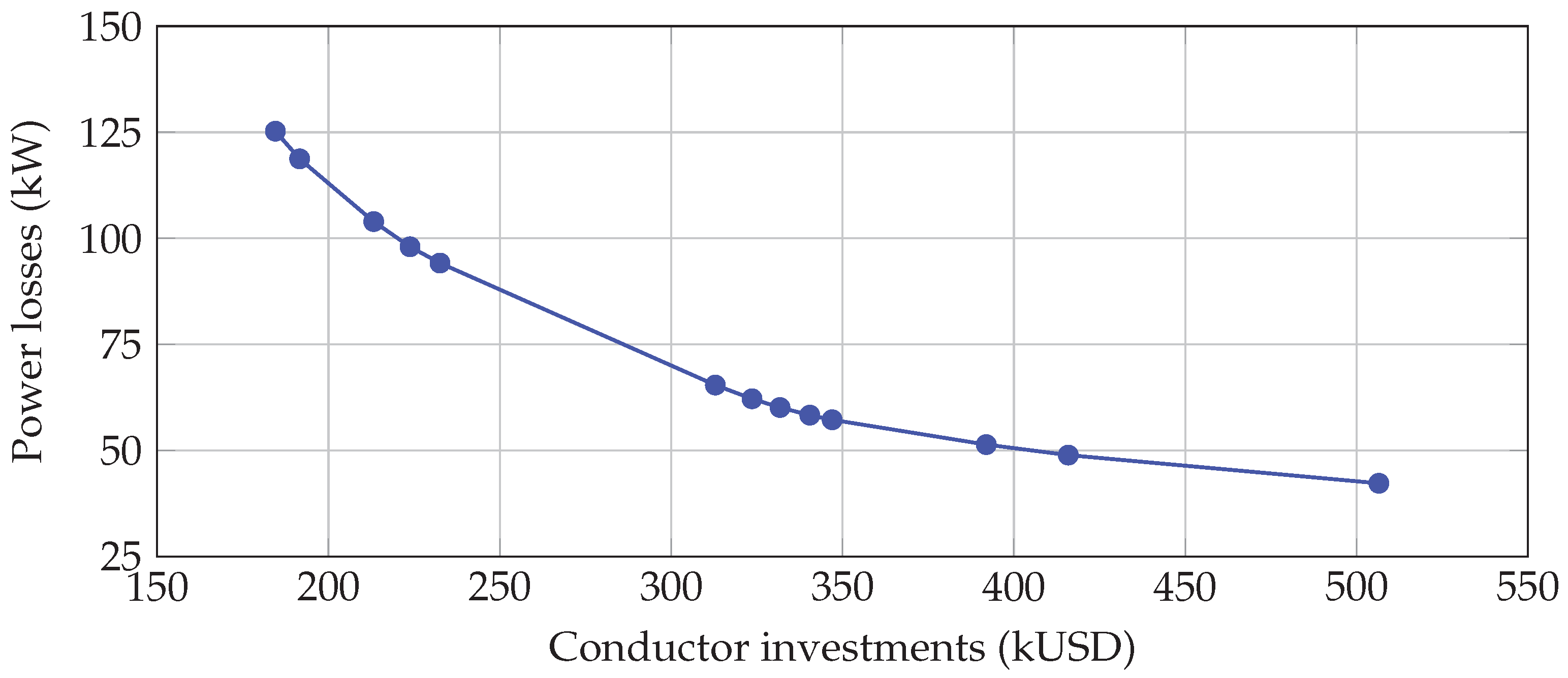
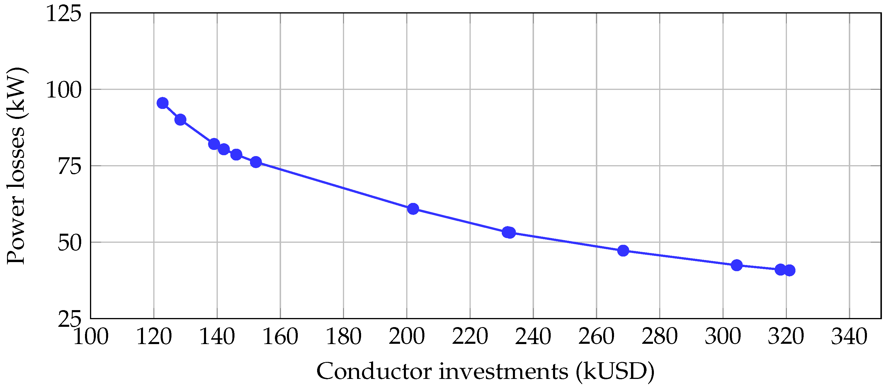
• There is an inverse relationship between the costs of energy losses ($z_1$) and conductor investment ($z_2$). As $\omega$ increases, greater priority is given to minimizing energy losses, leading to a significant reduction in $z_1$, albeit at the expense of higher investment costs. Conversely, lower values of $\omega$ prioritize the minimization of conductor investment costs, resulting in increased operational expenditure due to higher energy losses.
• The total objective function value ($z_1+z_2$) follows a nonmonotonic trend, with a minimum observed at $\omega =0.50$, where the total cost reached its lowest value: USD 550,680.21. This corresponds to the objective function of the single-objective optimization case, indicating that the best tradeoff between investment and energy losses costs occurs when both objectives are weighted equally. This suggests that neither extreme prioritization (low or high $\omega$) provides the most cost-effective solution.
• At $\omega =0.20$, the model strongly prioritized the minimization of conductor investment, resulting in a high energy losses cost of USD 457,519.23 but a relatively low investment cost (USD 184,516.28). However, the total objective function value remains high (USD 642,035.50), indicating that excessive emphasis on reducing initial expenditure can lead to inefficient long-term performance.
• As $\omega$ increased, energy losses costs decreased significantly, reaching USD 154,321.53 at $\omega =0.80$. However, the corresponding conductor investment rose to USD 506,506.13, leading to the highest total objective function value (USD 660,827.66). This suggests that excessive prioritization of energy losses minimization results in prohibitively high upfront costs.
• The lowest total cost was achieved at $\omega =0.50$, where the costs of investment and energy losses are well balanced. At this weighting, the cost of conductor investment is USD 227,087.16, while that of energy losses is USD 323,593.05, leading to an optimal total objective function value of USD 550,680.21. This result indicates that an equal prioritization of both objectives leads to the most economically efficient solution for the distribution company.

This analysis confirms that the multi-objective optimization approach effectively captures the tradeoffs between the costs of energy losses and conductor investment. The Pareto front demonstrates that extreme weightings lead to suboptimal cost configurations, whereas a balanced weighting ($\omega =0.50$) minimizes the total objective function value. These findings provide valuable insights for decision makers, suggesting that OCS should not solely focus on minimizing either energy losses or investment costs but rather seek a well-balanced compromise to ensure long-term economic efficiency in distribution system planning.

To illustrate the multi-objective nature of the OCS problem, Figure 4 presents the Pareto front for conductor investment and power losses in the 27-bus grid.

The behavior of this Pareto front indicates that the power loss variations for this test feeder ranged from $125.2475$ kW to $42.2461$ kW as the investments increased from their minimum to their maximum values. These results confirm the multi-objective nature of the OCS problem in electrical distribution grids. Furthermore, after an investment of approximately USD 312,892.50, energy losses tended to stabilize below 65.40 kW, with only minor variations beyond this point. This result suggests that the distribution company can formulate an investment plan based on the available conductor budget, aiming to minimize power losses as much as possible, which translates into reduced network operating costs.

5.2.2. The 33-Bus Grid

Table 9. Pareto front for the 33-bus system.

$\mathit{\omega }$	${\mathit{z}}_1$ (USD)	${\mathit{z}}_2$ (USD)	${\mathit{z}}_1+{\mathit{z}}_2$ (USD)
0.20	149,006.3712	321,016.3215	470,022.6927
0.25	149,893.2634	318,208.1384	468,101.4019
0.30	155,083.1649	304,338.0452	459,421.2101
0.35	172,512.9951	268,431.1886	440,944.1837
0.40	194,004.0224	232,622.4779	426,626.5003
0.45	194,590.0155	231,871.5890	426,461.6045
0.50	222,494.0963	201,987.5216	424,481.6179
0.55	278,375.9036	152,270.4034	430,646.3070
0.60	287,244.4779	146,073.3013	433,317.7791
0.65	293,640.0739	142,138.7573	435,778.8312
0.70	299,942.3727	139,055.1709	438,997.5436
0.75	329,054.1014	128,388.9880	457,443.0894
0.80	348,900.8846	122,772.6591	471,673.5437

presents the Pareto front obtained after solving the multi-objective optimization problem via the weighting-based optimization approach in the 33-bus feeder. The results highlight the tradeoffs between the expected annual cost of energy losses ($z_1$) and the investment made in conductors ($z_2$), providing a range of optimal solutions that balance these conflicting objectives.

The numerical results in Table 9 allow for the following observations:

• The results demonstrate an inverse relationship between the costs of energy losses ($z_1$) and conductor investment ($z_2$). As $\omega$ increases, the optimization strategy prioritizes the minimization of energy losses, leading to a significant reduction in $z_1$ at the expense of increased conductor investments. Conversely, smaller values of $\omega$ lead to a focus on minimizing $z_2$, resulting in higher operating costs due to increased losses.
• The total system cost ($z_1+z_2$) exhibits a nonmonotonic trend, with a minimum observed at $\omega =0.50$, where the total cost reached its lowest value (USD 424,481.61). This suggests that an equal weighting of investment and operating costs yields the most cost-effective solution. In contrast, extreme prioritization of either objective leads to suboptimal total costs.
• When $\omega =0.20$, the primary focus is on minimizing conductor investment costs, resulting in a low capital expenditure of USD 149,006.37, albeit at the expense of high energy losses costs (USD 321,016.32). Consequently, the total system cost remains relatively high (USD 470,022.69), highlighting the long-term inefficiencies of only prioritizing initial investment.
• At $\omega =0.80$, the optimization strategy strongly prioritized the reduction in energy losses, lowering $z_1$ to USD 122,772.65. However, this comes at the cost of significantly higher investment costs (USD 348,900.88), leading to a total system cost of USD 471,673.54, among the highest values observed. This confirms that an excessive prioritization of losses minimization results in prohibitively high upfront costs.
• The most cost-effective solution was achieved at $\omega =0.50$, where the conductor investment amounted to USD 201,987.52 and the energy losses to USD 222,494.09, yielding the lowest total system cost (USD 424,481.61). This balanced approach ensures economic efficiency by preventing excessive capital expenditure while maintaining manageable operating costs.

This analysis confirms that the multi-objective optimization approach effectively captures the tradeoffs between energy losses and investment costs. The Pareto front illustrates that extreme weightings lead to suboptimal cost structures, whereas a balanced weighting ($\omega =0.50$) minimizes the total expenditure. These findings provide valuable insights for decision makers in electrical distribution planning, emphasizing that conductor selection should not solely focus on minimizing either energy losses or investment costs but should instead aim for a well-balanced compromise to ensure long-term economic efficiency.

To illustrate the multi-objective nature of the OCS problem, Figure 5 presents the Pareto for conductor investment and power losses in the 33-bus grid.

These results confirm the multi-objective nature of the OCS problem for electrical distribution grids. In this context, the power losses ranged from $40.79$ kW to $95.51$ kW as the investment costs decreased from USD 321,016.32 to USD 122,772.66. For the distribution company, with a moderate investment of approximately USD 201,987.52, power losses can be reduced to around $60.91$ kW, which represents a reasonable tradeoff between investment costs and the expected level of energy losses.

5.3. Complementary Analysis

This subsection explores different aspects regarding the effective solution of the exact MINLP formulation associated with the OCS problem for electrical distribution networks. A larger-size test feeder was considered in this evaluation, i.e., the 69-bus grid. Like the 33-bus grid, it operates with 12,660 V at the terminals of the substation (line-to-ground), and it has 69 buses and 68 distribution lines. The main data on this test feeder are presented in

Table 10. Electrical parameters of the 69-bus grid.

Line l	Node k	Node m	${\mathit{L}}_{\mathit{l}}$ (km)	${\mathit{P}}_{\mathit{mt}}^{\mathit{d}}$ (kW)	${\mathit{Q}}_{\mathit{mt}}^{\mathit{d}}$ (kvar)	Line l	Node k	Node m	${\mathit{L}}_{\mathit{l}}$ (km)	${\mathit{P}}_{\mathit{mt}}^{\mathit{d}}$ (kW)	${\mathit{Q}}_{\mathit{mt}}^{\mathit{d}}$ (kvar)
1	1	2	0.1270	0	0	35	3	36	0.6948	26	18.55
2	2	3	0.9134	0	0	36	36	37	0.3171	26	18.55
3	3	4	0.6324	0	0	37	37	38	0.9502	0	0
4	4	5	0.0975	0	0	38	38	39	0.0344	24	17
5	5	6	0.2785	2.60	2.2	39	39	40	0.4387	24	17
6	6	7	0.5469	40.4	30	40	40	41	0.3816	102	1
7	7	8	0.9575	75	54	41	41	42	0.7655	0	0
8	8	9	0.9649	30	22	42	42	43	0.7952	6	4.3
9	9	10	0.1576	28	19	43	43	44	0.1869	0	0
10	10	11	0.9706	145	104	44	44	45	0.4898	39.22	26.3
11	11	12	0.9572	145	104	45	45	46	0.4456	39.22	26.3
12	12	13	0.4854	8	5	46	4	47	0.6463	0	0
13	13	14	0.8003	8	5	47	47	48	0.7094	79	56.4
14	14	15	0.1419	0	0	48	48	49	0.7547	384.7	274.5
15	15	16	0.4218	45	30	49	49	50	0.2760	384.7	274.5
16	16	17	0.9157	60	35	50	8	51	0.6797	40.5	28.3
17	17	18	0.7922	60	35	51	51	52	0.6551	3.6	2.7
18	18	19	0.9595	0	0	52	9	53	0.1626	4.35	3.5
19	19	20	0.6557	1	0.6	53	53	54	0.1190	26.4	19
20	20	21	0.0357	114	81	54	54	55	0.4984	24	17.2
21	21	22	0.8491	5	3.5	55	55	56	0.9597	0	0
22	22	23	0.9340	0	0	56	56	57	0.3404	0	0
23	23	24	0.6787	28	20	57	57	58	0.5853	0	0
24	24	25	0.7577	0	0	58	58	59	0.2238	100	72
25	25	26	0.7431	14	10	59	59	60	0.7513	0	0
26	26	27	0.3922	14	10	60	60	61	0.2551	1244	888
27	3	28	0.6555	26	18.6	61	61	62	0.5060	32	23
28	28	29	0.1712	26	18.6	62	62	63	0.6991	0	0
29	29	30	0.7060	0	0	63	63	64	0.8909	227	162
30	30	31	0.0318	0	0	64	64	65	0.9593	59	42
31	31	32	0.2769	0	0	65	11	66	0.5472	18	13
32	32	33	0.0462	10	10	66	66	67	0.1386	18	13
33	33	34	0.0971	14	14	67	12	68	0.1493	28	20
34	34	35	0.8235	4	4	68	68	69	0.2575	28	20

and Figure 6.

Note that for this test feeder, the same set of candidate conductor gauges reported in Table 5 was employed.

Table 11. Numerical results for the 69-bus grid after solving the exact MINLP formulation.

Method	Gauges	Investment (USD)	Losses (USD)	Annual Cost (USD)
MINLP	$\left[\begin{array}{c}7,7,7,7,7,7,7,7,3,2,1,1,1,1,\\ 1,1,1,1,1,1,1,1,1,1,1,1,1,1,\\ 1,1,1,1,1,1,1,1,1,1,1,1,1,1,\\ 1,1,1,3,3,3,1,1,1,5,5,5,5,5,\\ 5,5,4,4,1,1,1,1,1,1,1,1\end{array}\right]$	583,287.3411	374,253.2969	957,540.6380

presents the numerical results obtained for the 69-bus grid after solving the MINLP model in the Julia software.

The solution regarding the optimal conductor size is expressed in terms of gauge assignments for each line segment, where larger gauge values are allocated to specific sections of the network, likely due to higher current flow requirements. The total investment cost associated with the selected conductor sizes amounted to USD 583,287.34, while the cost of power losses over the period of operation was estimated at USD 374,253.30. Consequently, the overall annual cost, which integrates both investment and energy losses, reached USD 957,540.64. These results highlight the tradeoff between initial infrastructure investment and long-term operating costs, emphasizing the importance of an OCS strategy to minimize total expenditure.

5.3.1. Processing Times

To evaluate the computational efficiency of the proposed solution methodology, which combines the B&B method with an IPO, 100 consecutive evaluations were performed for each test feeder.

Table 12. Processing times required for solving the exact MINLP formulation of the OCS problem.

Test Feeder	Minimum (s)	Maximum (s)	Average (s)
27-bus	17.0910	18.7730	17.8780
33-bus	26.6140	26.6390	26.6219
69-bus	185.2049	189.9939	189.5480

presents the average processing times along with their corresponding minimum and maximum values.

An analysis of these processing times reveals the following:

• The 27-bus system exhibited the lowest computational burden, with an average processing time of approximately 17.88 s and a small variation between its minimum (17.09 s) and maximum (18.77 s) values.
• The 33-bus system maintained relatively stable processing times, with an average of 26.62 s and a narrow range (26.61 s to 26.64 s), indicating a consistent performance.
• The 69-bus system experienced significantly higher computational demands, with an average processing time of 189.54 s. The variation between its minimum (185.20 s) and maximum (189.99 s) values suggests a more complex problem structure, leading to slight fluctuations.

These results indicate that the computational effort increases alongside the system size, as is expected with MINLP problems. While the 27- and 33-bus cases exhibited relatively low and stable processing times, the 69-bus system showed a significantly higher computational burden. However, considering that the solution space of the 69-bus system is substantially larger than that of the 33- and 27-bus grids, the average processing times remain reasonable. This is acceptable, given that the problem being solved pertains to planning optimization, which does not require real-time solutions in practical implementation.

5.3.2. Impact of Dispersed Generation

To assess the impact of dispersed generation on the proposed MINLP formulation, the 69-bus grid was analyzed after incorporating three DERs within the distribution network [30]. These sources were installed at buses 18, 50, and 61, with capacities of 580 kvar, 715 kvar, and 1220 kvar, respectively. Three power factor scenarios were considered for these generation sources, i.e., unitary (1.0), 0.90 lagging, and 0.80 lagging, allowing them to support or inject reactive power into the system. It is important to note that these sources were dispatched at their full capacity.

Table 13. Numerical results for the 69-bus grid for different power factor assessments.

Power Factor	Gauges	Investment (USD)	Losses (USD)	Annual Cost (USD)
1.00	$\left[\begin{array}{c}7,7,7,7,7,7,7,7,3,2,1,1,1,1,\\ 1,1,1,1,1,1,1,1,1,1,1,1,1,1,\\ 1,1,1,1,1,1,1,1,1,1,1,1,1,1,\\ 1,1,1,3,3,3,1,1,1,5,5,5,5,5,\\ 5,5,4,4,1,1,1,1,1,1,1,1\end{array}\right]$	403,037.6340	252,705.9665	655,743.6029
0.90	$\left[\begin{array}{c}5,5,4,4,4,4,4,4,1,1,1,1,1,1,\\ 1,1,1,1,1,1,1,1,1,1,1,1,1,1,\\ 1,1,1,1,1,1,1,1,1,1,1,1,1,1,\\ 1,1,1,1,1,1,1,1,1,3,3,2,2,2,\\ 2,2,2,2,1,1,1,1,1,1,1,1\end{array}\right]$	277,539.6204	204,136.9978	481,676.6182
0.80	$\left[\begin{array}{c}7,7,7,7,7,7,7,7,3,2,1,1,1,1,\\ 1,1,1,1,1,1,1,1,1,1,1,1,1,1,\\ 1,1,1,1,1,1,1,1,1,1,1,1,1,1,\\ 1,1,1,3,3,3,1,1,1,5,5,5,5,5,\\ 5,5,4,4,1,1,1,1,1,1,1,1\end{array}\right]$	274,246.2636	191,533.7978	465,780.0614

presents the numerical results for the 69-bus system under different power factors while considering the integration of DERs. The following key observations can be made:

• The incorporation of DERs significantly affects both investment and operating costs. As the power factor shifted from 1.00 (unitary) to 0.80 lagging, there was a notable reduction in both values. The total annual cost decreased from USD 655,743.60 at a unitary power factor to USD 465,780.06 at 0.80 lagging, representing a 29.0% reduction. This demonstrates the role of reactive power support in minimizing the overall system costs.
• The gauge selection varies with the power factor scenario. With a unitary power factor, larger conductor sizes (e.g., gauge 7) were predominant, particularly in the main feeder sections, due to higher current demands. However, as the power factor decreased to 0.90 and 0.80 lagging, smaller conductor sizes (e.g., gauges 4 and 5) became prevalent. This indicates that improved reactive power support reduces current magnitudes, thereby enabling the use of smaller conductors and lowering investment costs.
• Lower power factors improve the system’s ability to locally manage reactive power, leading to a 24.2% reduction in the cost of energy losses, from USD 252,705.97 at a unitary power factor to USD 191,533.80 at 0.80 lagging. This suggests that allowing DERs to inject reactive power optimizes power flows, reduces voltage drops, and enhances the overall system efficiency.
• The results confirm that balancing the costs of investment with those of energy losses is crucial. With a unitary power factor, higher investment costs led to increased conductor sizes, yet the system experienced higher operating costs due to greater energy losses. Conversely, at 0.80 lagging, the lowest annual cost was achieved, demonstrating that incorporating reactive power compensation into DER operation significantly reduces the long-term economic burden of distribution networks.

These results validate the economic and technical advantages of integrating DERs with reactive power support into distribution networks. The ability to operate at a 0.80 lagging power factor led to the most cost-effective solution, minimizing the costs of both conductor investment and energy losses. These findings highlight the necessity of optimizing DER operation to fully exploit their potential in improving the efficiency and reliability of electrical distribution systems.

6. Conclusions and Future Work

This study analyzed the single- and multi-objective optimal conductor selection problem for 27- and 33-bus distribution networks, as well as single-objective analysis with DERs integration in the 69-bus grid, leading to the following key conclusions:

• There is a clear tradeoff between the costs of conductor investment ($z_2$) and those of energy losses ($z_1$). Lower upfront costs result in higher long-term operational expenditure, while prioritizing losses minimization increases initial costs. Thus, a balanced optimization approach is essential for cost-effective planning.
• The Pareto front analysis indicates that an equal weighting of both objectives ($\omega =0.50$) yields the most cost-effective solution, minimizing the total costs to USD 550,680.21 in the 27-bus grid and to USD 424,481.62 in the 33-bus feeder. This balance ensures economic efficiency without excessive prioritization of either cost.
• The sensitivity analysis of different weightings confirms that extreme prioritization leads to suboptimal results. Weighting strategies favoring either investment cost minimization ($\omega =0.20$) or losses minimization ($\omega =0.80$) led to disproportionate cost increases in the other component.
• The results for the 69-bus grid demonstrate that integrating DERs with reactive power support significantly reduces both investment and operating costs. As the power factor shifts from a unitary one to 0.80 lagging, the total annual cost decreased by 29.0%, while the energy loss costs dropped by 24.2%. The conductor gauge selection adapts to improved reactive power compensation, enabling the use of smaller conductors and further reducing investment costs. These findings highlight the economic and technical benefits of optimizing DER operation, emphasizing its role in improving distribution network efficiency and cost-effectiveness.

Future research will focus on extending the optimization model to incorporate distributed renewable energy sources (e.g., photovoltaic systems) in order to evaluate their impact on conductor selection and overall network efficiency under real-world operating conditions. Additionally, the influence of dynamic load variations and demand-side management strategies will be explored by integrating real-time data analytics and probabilistic forecasting techniques to enhance conductor sizing decisions. Another key direction could involve the development of hybrid methodologies that combine exact mathematical optimization with advanced metaheuristic algorithms, aiming to improve computational efficiency while ensuring optimal solutions in large-scale distribution networks. Furthermore, the proposed optimization framework will be validated using real distribution network data while considering geographical constraints, regulatory policies, and practical implementation challenges, with the purpose of assessing its feasibility in real-world applications. The MINLP formulation will also be adapted to address scenarios where the distribution network is partially constructed, integrating conductor replacement strategies to the evaluate tradeoffs between reusing existing infrastructure and deploying new conductors. Lastly, the methodology will be expanded to incorporate additional real-world constraints such as network reconfiguration options, operational reliability considerations, and phased expansion planning, thus ensuring broader applicability in practical distribution system planning. These advancements will contribute to the continuous development of efficient and robust optimization models, allowing for more effective planning and operation of modern electrical distribution networks.

References

- Haben, S.; Voss, M.; Holderbaum, W. Primer on Distribution Electricity Networks. In Core Concepts and Methods in Load Forecasting; Springer International Publishing: Cham, Switzerland, 2023; pp. 13–22. [Google Scholar] [CrossRef]
- Daccò, E.; Falabretti, D.; Ilea, V.; Merlo, M.; Nebuloni, R.; Spiller, M. Decentralised Voltage Regulation through Optimal Reactive Power Flow in Distribution Networks with Dispersed Generation. Electricity 2024, 5, 134–153. [Google Scholar] [CrossRef]
- Muhammad Ridzuan, M.I.; Mohd Fauzi, N.F.; Roslan, N.N.R.; Mohd Saad, N. Urban and rural medium voltage networks reliability assessment. SN Appl. Sci. 2020, 2, 241. [Google Scholar] [CrossRef]
- Petinrin, J.; Shaabanb, M. Impact of renewable generation on voltage control in distribution systems. Renew. Sustain. Energy Rev. 2016, 65, 770–783. [Google Scholar] [CrossRef]
- Gallegos, J.; Arévalo, P.; Montaleza, C.; Jurado, F. Sustainable Electrification—Advances and Challenges in Electrical-Distribution Networks: A Review. Sustainability 2024, 16, 698. [Google Scholar] [CrossRef]
- Pengwah, A.B.; Fang, L.; Razzaghi, R.; Andrew, L.L.H. Topology Identification of Radial Distribution Networks Using Smart Meter Data. IEEE Syst. J. 2022, 16, 5708–5719. [Google Scholar] [CrossRef]
- Montoya, O.D.; Serra, F.M.; De Angelo, C.H.; Chamorro, H.R.; Alvarado-Barrios, L. Heuristic Methodology for Planning AC Rural Medium-Voltage Distribution Grids. Energies 2021, 14, 5141. [Google Scholar] [CrossRef]
- Hamidan, M.A.; Borousan, F. Optimal planning of distributed generation and battery energy storage systems simultaneously in distribution networks for loss reduction and reliability improvement. J. Energy Storage 2022, 46, 103844. [Google Scholar] [CrossRef]
- Vélez-Marín, V.M.; Montoya, O.D.; Hernández, J.C. A DIgSILENT Programming-Based Approach for Selecting Conductors in Distribution Networks via the Tabu Search Algorithm. In Proceedings of the 2024 IEEE Colombian Conference on Applications of Computational Intelligence (ColCACI), Pamplona, Colombia, 17–19 July 2024; pp. 1–6. [Google Scholar] [CrossRef]
- Ponce, D.; Aguila Téllez, A.; Krishnan, N. Optimal Selection of Conductors in Distribution System Designs Using Multi-Criteria Decision. Energies 2023, 16, 7167. [Google Scholar] [CrossRef]
- Martínez-Gil, J.F.; Moyano-García, N.A.; Montoya, O.D.; Alarcon-Villamil, J.A. Optimal Selection of Conductors in Three-Phase Distribution Networks Using a Discrete Version of the Vortex Search Algorithm. Computation 2021, 9, 80. [Google Scholar] [CrossRef]
- Ismael, S.M.; Aleem, S.H.E.A.; Abdelaziz, A.Y. Optimal selection of conductors in Egyptian radial distribution systems using sine-cosine optimization algorithm. In Proceedings of the 2017 Nineteenth International Middle East Power Systems Conference (MEPCON), Cairo, Egypt, 19–21 December 2017. [Google Scholar] [CrossRef]
- Nivia Torres, D.J.; Salazar Alarcón, G.A.; Montoya Giraldo, O.D. Optimal Selection of Conductors in Three-Phase Distribution Networks using the Newton Metaheuristic Algorithm. Ingeniería 2022, 27, e19303. [Google Scholar] [CrossRef]
- Montoya, O.D.; Garces, A.; Castro, C.A. Optimal Conductor Size Selection in Radial Distribution Networks Using a Mixed-Integer Non-Linear Programming Formulation. IEEE Lat. Am. Trans. 2018, 16, 2213–2220. [Google Scholar] [CrossRef]
- Mandal, S.; Pahwa, A. Optimal Selection of Conductors for Distribution Feeders. IEEE Power Eng. Rev. 2002, 22, 71. [Google Scholar] [CrossRef]
- Gallego Pareja, L.A.; López-Lezama, J.M.; Gómez Carmona, O. A MILP Model for Optimal Conductor Selection and Capacitor Banks Placement in Primary Distribution Systems. Energies 2023, 16, 4340. [Google Scholar] [CrossRef]
- Farrag, M.A.; Khalil, A.H.; Omran, S. Optimal conductor selection and capacitor placement in radial distribution system using nonlinear AC load flow equations and dynamic load model. Int. Trans. Electr. Energy Syst. 2020, 30, e12316. [Google Scholar] [CrossRef]
- Gallego Pareja, L.A.; López-Lezama, J.M.; Gómez Carmona, O. Enhancing power distribution performance through simultaneous optimization of voltage regulators placement and conductor selection: A multi-period MILP approach. Results Eng. 2025, 25, 104311. [Google Scholar] [CrossRef]
- Kroger, O.; Coffrin, C.; Hijazi, H.; Nagarajan, H. Juniper: An Open-Source Nonlinear Branch-and-Bound Solver in Julia. In Integration of Constraint Programming, Artificial Intelligence, and Operations Research; Springer International Publishing: Cham, Switzerland, 2018; pp. 377–386. [Google Scholar] [CrossRef]
- Scavuzzo, L.; Aardal, K.; Lodi, A.; Yorke-Smith, N. Machine learning augmented branch and bound for mixed integer linear programming. Math. Program. 2024. [Google Scholar] [CrossRef]
- Borchers, B. MINLP: Branch and Bound Methods. In Encyclopedia of Optimization; Springer: Boston, MA, USA, 2008; pp. 2138–2142. [Google Scholar] [CrossRef]
- Androulakis, I.P. MINLP: Branch and Bound Global Optimization Algorithm. In Encyclopedia of Optimization; Springer: Boston, MA, USA, 2001; pp. 1415–1421. [Google Scholar] [CrossRef]
- Benson, H.Y. Mixed integer nonlinear programming using interior-point methods. Optim. Methods Softw. 2011, 26, 911–931. [Google Scholar] [CrossRef]
- Benson, H.Y. Using Interior-Point Methods within an Outer Approximation Framework for Mixed Integer Nonlinear Programming. In Mixed Integer Nonlinear Programming; Springer: New York, NY, USA, 2011; pp. 225–243. [Google Scholar] [CrossRef]
- Lubin, M.; Dowson, O.; Dias Garcia, J.; Huchette, J.; Legat, B.; Vielma, J.P. JuMP 1.0: Recent improvements to a modeling language for mathematical optimization. Math. Program. Comput. 2023, 15, 581–589. [Google Scholar] [CrossRef]
- Pal, S.; Bhattacharya, M.; Dash, S.; Lee, S.S.; Chakraborty, C. A next-generation dynamic programming language Julia: Its features and applications in biological science. J. Adv. Res. 2024, 64, 143–154. [Google Scholar] [CrossRef]
- Bezanson, J.; Edelman, A.; Karpinski, S.; Shah, V.B. Julia: A fresh approach to numerical computing. SIAM Rev. 2017, 59, 65–98. [Google Scholar] [CrossRef]
- Huangfu, Q.; Hall, J.A.J. Parallelizing the dual revised simplex method. Math. Program. Comput. 2017, 10, 119–142. [Google Scholar] [CrossRef]
- Marler, R.T.; Arora, J.S. The weighted sum method for multi-objective optimization: New insights. Struct. Multidiscip. Optim. 2009, 41, 853–862. [Google Scholar] [CrossRef]
- Kaur, S.; Kumbhar, G.; Sharma, J. A MINLP technique for optimal placement of multiple DG units in distribution systems. Int. J. Electr. Power Energy Syst. 2014, 63, 609–617. [Google Scholar] [CrossRef]