Implementation of Autonomous Navigation for Solar-Panel-Cleaning Vehicle Based on YOLOv4-Tiny ^†

Abstract

We developed an autonomous navigation system for a solar-panel-cleaning vehicle. The system utilizes the YOLOv4-Tiny object detection model to detect white lines on the solar panels and combines the model with a proportional–integral–derivative (PID) controller to achieve autonomous navigation functionality. The main system platform was built on Raspberry Pi, and the Intel Neural Compute Stick 2 (NCS2) was used for hardware acceleration, which boosted the model’s inference speed from 2 to 8 frames per second (FPS), significantly enhancing the system’s real-time performance. By tuning the PID controller parameters, the system achieved an optimal performance, with $K_P$ = 11, $K_i$ = 0.01, and $K_d$ = 30, maintaining the average value of the error e(t) at −0.0412 and the standard deviation at 0.1826 and improving the inference speed. The system autonomously followed the white lines on the solar panels and automatically turned when reaching the boundaries. The system also autonomously cleaned itself. The developed autonomous navigation system effectively improved the efficiency and convenience of solar panel cleaning.

1. Introduction

Solar energy, as a clean and renewable energy source, plays a crucial role in the global transition of the energy structure. Solar panels, as the core equipment of solar power generation, have are highly efficient at converting and utilizing energy. With the growing global demand for renewable energy, the installation of solar panels is rapidly increasing. However, dirt, dust, bird droppings, and other pollutants accumulate on the surface of solar panels, significantly reducing their energy conversion efficiency. Therefore, keeping solar panels clean is essential for improving their performance and extending their lifespan.

The solar-panel-cleaning vehicle is designed for cleaning solar panels and removing contaminants such as dust, dirt, and oil films to improve their power generation efficiency. This vehicle is equipped with a high-pressure water jet and a cleaning liquid pump which sprays high-pressure water and clean liquid onto the solar panels for cleaning. Additionally, it is equipped with a safe and stable suspension system to easily adapt to different terrains and tilt angles, as shown in Figure 1 [1].

For the convenient remote controlling of the solar-panel-cleaning vehicle, the autonomous navigation function is essential to move on solar panels. Automatic cleaning functionality is also necessary to improve cleaning efficiency and operational convenience. Figure 2 illustrates the autonomous navigation of the solar-panel-cleaning vehicle. Generally, the autonomous navigation function requires addressing the positioning issue. A positioning system is employed to locate an object in space, including interstellar, global, and regional systems in a broad area. Positioning systems are classified into indoor positioning systems (IPSs) and outdoor positioning systems (OPSs) [2]. The most common outdoor positioning system is the global positioning system (GPS) developed by the U.S. government. Its main advantages include high signal penetration, global coverage of 98%, high efficiency, and wide-ranging applications. Its positioning accuracy ranges from 0.3 to 6 m [3]. Indoor positioning systems are commonly used in buildings and basements with technologies such as WiFi, radio-frequency identification (RFID), inertial measurement units (IMUs), and simultaneous localization and mapping (SLAM) [4]. Since solar panels are used outdoors, an outdoor positioning system must be adopted. However, GPS is not appropriate for the positioning of the solar-panel-cleaning vehicle due to the limitations of current outdoor positioning accuracy, so a line-following navigation mode was used instead.

Due to the presence of parallel white lines on the solar panels, we used YOLOv4-Tiny [5] to detect the parallel white lines and a proportional–integral–derivative (PID) controller to achieve autonomous navigation [6]. When the solar-panel-cleaning vehicle reaches the boundary, it turns around and continues to move in a straight line in the opposite direction, until the cleaning is completed or the autonomous navigation function is deactivated.

2. System Flowchart

Figure 3 shows the system flowchart. After the autonomous navigation function is activated, the system loads the YOLOv4-Tiny model. Next, it detects the boundary using boundary sensors. If the boundary is not reached, the camera captures images, and white line detection is performed on the input images. The system calculates the error e(t) between the x-coordinate of the detected white line and the x-coordinate of the image center. It then calculates the integral of the error e(t) over time and the rate of change in the error e(t) for time. These three factors are combined to control the speed of the left and right wheels of the solar-panel-cleaning vehicle for autonomous navigation. If the boundary is reached, the autonomous navigation function is paused, and the vehicle turns. For the odd-numbered rows, it moves forward one vehicle length, rotates 90° clockwise, moves forward another vehicle length, and then rotates 90° clockwise again. For the even-numbered rows, it reverses by one vehicle length, rotates 90° counterclockwise, moves forward one vehicle length, and then rotates 90° counterclockwise again.

3. Methods

3.1. White Line Detection Based on YOLOv4-Tiny

The white line refers to the line observed on the solar panel when the camera captures a top-down view of the panel, as shown in Figure 4. The solar panel exhibits distinct parallel stripes and one relatively wider parallel white line.

White lines are detected using computer vision and deep learning-based object detection algorithms involving convolutional neural networks (CNNs). Recently, object detection algorithms have evolved into accurate and fast systems and have been widely applied in academia and industry. Among the various methods, YOLO stands out due to its fast approach. This method was introduced by Redmon in 2016 [7]. In this study, a simplified version of YOLOv4, known as YOLOv4-Tiny, was selected as the white line detector as it reduces the computational requirements, while sacrificing accuracy, which is appropriate for embedded applications.

By using a pre-trained YOLO model to detect white lines, the actual detection results are shown in Figure 5. To detect the white lines marked with a bounding box, the number inside the box represents the confidence level of the detected object. This is an example of the white line detection result.

3.2. PID Controller

The PID controller was originally used to improve the steering control system of the battleship USS New Mexico [6]. Presently, the PID controller is applied in industrial machines. Additionally, it is also used in cruise control systems for cars and trucks. The PID controller adjusts the control output based on proportional, integral, and derivative control methods. Proportional control adjusts the control output based on the difference between the target and the actual value. When moving straight along the white line, the target value is the x-coordinate of the center of the image, and the actual value is the x-coordinate of the white line at time t. Therefore, the error at time t is expressed as e(t). The output of the proportional controller is proportional to the error, and the proportional constant $K_p$ is used to determine the extent of the error’s impact on the system. For moving straight along the white line, if $K_p$ is too large, small errors are amplified, and the cleaning vehicle sways. Conversely, if $K_p$ is too small, the vehicle’s correction speed decreases. The equation for proportional control is (1).

$$P\left(t\right)=K_p\cdot e\left(t\right)$$

(1)

The integral controller considers the accumulated error over time to eliminate the steady-state error. The integral part adjusts the control output by integrating the error over time, and the integral constant $K_i$ is used to determine how quickly the system eliminates the steady-state error. Integral control ensures that the final error approaches zero, but an excessively high error causes the system to overcorrect or become unstable. The equation for integral control is (2).

$$I\left(t\right)=K_i\cdot {\int }_0^{t}e\left(\tau \right) d\tau$$

(2)

The derivative controller adjusts the control output based on the rate of change in the error to predict the error’s trend and make pre-emptive corrections. The derivative constant, $K_d$ is used to determine the extent to which the error’s rate of change affects the system. An appropriate $K_d$ reduces system overshooting and oscillation, but an excessively high $K_d$ makes the system sensitive. The equation for derivative control is (3).

$$D\left(t\right)=K_d\cdot {\displaystyle \frac{de\left(t\right)}{dt}}$$

(3)

The complete equation for the PID controller is (4), in which the advantages of all the three components are combined to achieve the precise control of the signal u(t).

$$u\left(t\right)=P\left(t\right)+I\left(t\right)+D\left(t\right)$$

(4)

4. Results and Discussions

Due to the large size of the commercial solar-panel-cleaning vehicle, we used a two-wheeled robot with a similar structure as a solar-panel-cleaning vehicle. The system’s main platform was Raspberry Pi. When performing YOLOv4-Tiny model inference using the CPU, the system processed two images per second on average. To increase the inference speed, we used Neural Compute Stick 2 (NCS2) acceleration hardware [8] that processed eight images per second with NCS2.

NCS2 is an artificial intelligence (AI) acceleration hardware developed by Intel. NCS2 is a compact device based on USB 3.0 (Figure 6). It contains Intel’s Movidius Myriad X VPU, a hardware accelerator specifically designed for deep learning and visual processing. NCS2 can be used with any device running Windows, Linux, macOS, or Raspbian. These devices operate on Intel’s OpenVINO toolkit [9] to optimize neural networks and deploy them on multiple NCS2 units. The key feature of NCS2 is its ability to accelerate the inference process of various deep learning models. Due to its small size and low power consumption, NCS2 is a powerful, yet affordable solution for accelerating neural networks. NCS2 has been utilized in areas such as smart home systems, video surveillance systems for home or small offices, and other tasks.

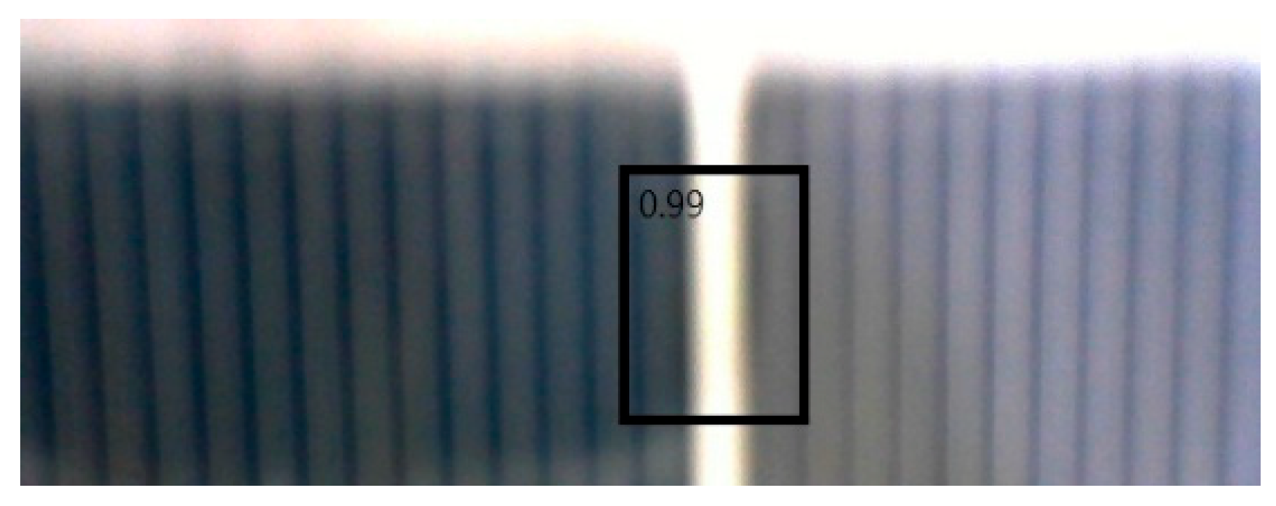
In application scenarios, a camera mounted on a solar-panel-cleaning vehicle is used to capture images from a bird’s eye view and film the scene. In operation, white lines may appear at any position within the image. Due to deviations in the vehicle’s straight line movement, the white lines tilt either left or right. Since YOLO is a supervised learning model that requires labeled targets, bounding boxes are used for annotation in YOLO. In the image dataset, 110 images with a resolution of 640 × 240 pixels were selected in this study. In sample images (Figure 7a–e), each white line was manually annotated with a bounding box (Figure 7f–j). The annotation process was carried out using Labelme software [11].

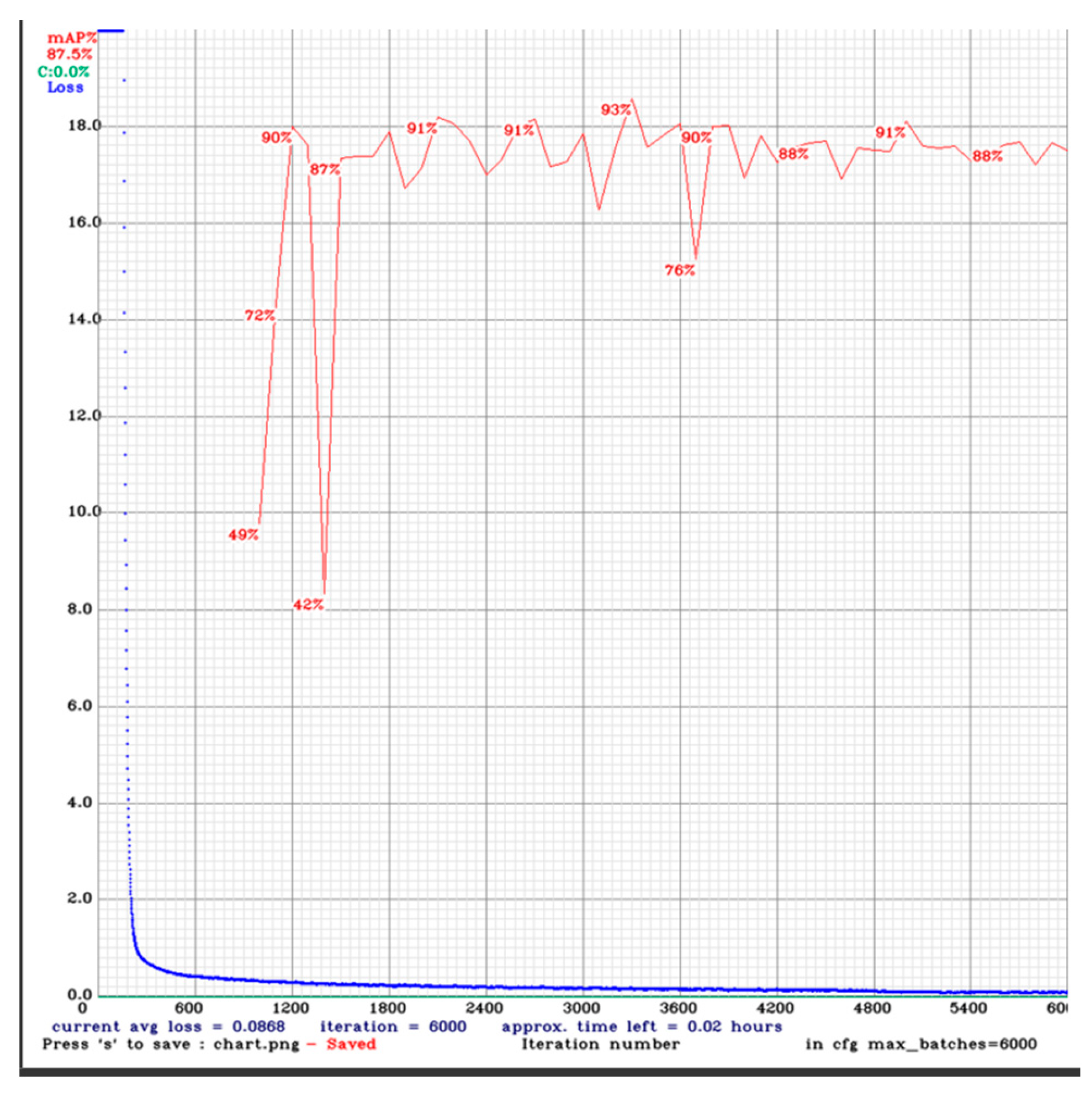
In model training, the learning rate was set to 0.00261, and the momentum was set to 0.9. The model was trained for 6000 epochs, with a batch size of 32. The model’s performance was evaluated using average precision (AP@0.5), where AP@0.5 refers to the AP detected when the true positive IOU threshold was set to 0.5. The performance of YOLOv4-Tiny in white line detection is shown in Figure 8. In the experiment, 90% of the solar panel images were randomly selected for training, while the remaining 10% were used for testing. The model’s average loss began to stabilize around 1200 epochs, and it achieved the highest AP of approximately 93% at around 3500 epochs.

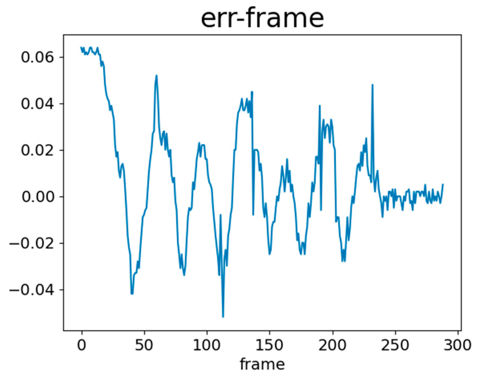
To evaluate the actual path of the vehicle, we recorded the vehicle’s e(t) during its movement. e(t) represents the difference between the white line position x at time t and the target position x, normalized within ±1. When the vehicle moved in a straight line on the solar panels, e(t) was monitored to track the deviation of the vehicle. Figure 9 and Figure 10 show e(t) without using NCS2 and with NCS2, respectively. These figures represent the changes in e(t) as the vehicle travelled along a straight path. When the model inferred white lines without using NCS2, the fluctuations in e(t) were significant, with a maximum error reaching 0.9. However, when NCS2 was used for model inference, the variations in e(t) became smaller, remaining within a stable range of ±0.06. This difference occurred because the speed of model inference affected the accuracy of the vehicle’s corrections using the PID controller. When inference is slow, real-time adjustments cannot be made. Additionally, with NCS2, e(t) stabilized after about 250 frames, whereas the maximum frame count was 60 without NCS2 due to delayed inference. Such inference caused incorrect PID control adjustments, leading the vehicle off the path and preventing it from detecting the white line.

PID control was adjusted using the proportional constant, $K_P$, the integral constant $K_i$, and the derivative constant $K_d$. The average value and standard deviation of e(t) were monitored for each set of conditions. The performance of the PID controller largely depends on the proper tuning of these parameters. By adjusting $K_P$, $K_i$, and $K_d$, the system conducted optimal control to meet various control requirements.

The experimental results for $K_P$ are shown in

Table 1. Experimental results of proportional parameter $K_P$.

${\mathit{K}}_{\mathit{P}}$	Average Value of e(t)	Standard Deviation of e(t)
7.5	−0.1587	0.1866
11	−0.0533	0.2264
15	−0.0837	0.1958

. When $K_P$ increased from 7.5 to 11, the average value of e(t) significantly decreased. However, when $K_P$ increased to 15, the average value of e(t) slightly increased. The standard deviation of e(t) was highest when $K_P$ was 11, though the increase was not substantial. By balancing the average value and standard deviation of e(t), the optimal proportional constant $K_P$ was determined to be 11. Considering the results, the experiments were conducted on $K_i$ with $K_P$ of 11.

The experimental results for ${ K}_i$ are shown in

Table 2. Experimental results of integral parameter $K_i$.

${\mathit{K}}_{\mathit{i}}$	Average Value of e(t)	Standard Deviation of e(t)
0.1	−0.0151	0.3576
0.01	−0.0653	0.2134
0.001	−0.0683	0.2380

. When ${ K}_i$ was 0.1, the average value of e(t) became the smallest, but the standard deviation of e(t) became large, indicating greater variability in the overall error. When ${ K}_i$ was reduced to 0.01, the average value and standard deviation of e(t) reached a better balance. However, when ${ K}_i$ was further reduced to 0.001, the average and standard deviation of e(t) increased. Considering the result, the experiments were conducted on $K_d$ with $K_P$ set to 11 and $K_i$ set to 0.01.

The experimental results for $K_d$ are shown in

Table 3. Experimental results of derivative parameter $K_d$.

${\mathit{K}}_{\mathit{d}}.$	Average Value of e(t)	Standard Deviation of e(t)
10	−0.0854	0.2245
30	−0.0412	0.1826
50	−0.1422	0.1956

. When $K_d$ was 10, the average and standard deviation of e(t) tended to be large. As $K_d$ increased to 30, the average value and standard deviation of e(t) decreased, which showed the best $K_d$. However, when $K_d$ increased to 50, the average value of e(t) increased, indicating that the system had become overly sensitive.

By adjusting and experimenting with the proportional, integral, and derivative parameters of the PID controller, the optimal proportional parameter $K_P$ was determined as 11, the optimal integral parameter $K_i$ was 0.01, and the optimal derivative parameter $K_d$ was 30. Under these PID control parameters, the entire navigation system became stable, and the average value and standard deviation of e(t) reached their lowest values of −0.0412 and 0.1826, respectively.

To adjust the parameters of the PID controller, the vehicle was tested while moving along a straight line. The adjusted PID controller system was tested on a complete standard solar panel path (Figure 2). As shown in Figure 3, navigation was performed through white line detection and PID control until the boundary was reached. Upon encountering the boundary, the system performed reversing, turning 90°, moving forward, and turning back 90°. The 90° turns were controlled over time. After turning, e(t) significantly increased, as depicted in Figure 11. In the figure, the red points indicate the recorded values of e(t) after completing the sequence of reversing, turning 90°, moving forward, and turning back 90°. A larger e(t) implies that the system requires more time to stabilize the value of e(t). To address this, the time-controlled turns were replaced with angle-controlled turns. The e(t) values after completing the path with angle-controlled turns are shown in Figure 12, demonstrating an effective reduction in post-turn e(t). e(t) after the series of turns was maintained within a range of ±0.25.

The angle calculation relies on the MPU-6050 six-axis sensor [12]. The appearance of the MPU-6050 is shown in Figure 13. It contains a three-axis accelerometer and a gyroscope to measure the acceleration and angular velocity of an object. Acceleration is the rate of change in an object’s velocity over time, and angular velocity is the rate of change in an object’s angle during rotation. By measuring acceleration and the rotational angle on different axes, the tilt angle, the movement direction, and the rotational angle of the object were calculated. The angle used in angle-controlled turning is the rotational angle and is calculated using (5).

$$\theta (t)=\theta (0)+{\int }_0^t\omega \left(t\right) dt$$

(5)

where θ(0) is the rotational angle at time t, and θ(0) is the initial angle, which is usually assumed to be 0. ω(t) represents angular velocity at time t, which is the rate of change in the angle. By integrating angular velocity from time 0 to t, the angle over this period is obtained.

5. Conclusions

We developed an autonomous navigation system for a solar-panel-cleaning vehicle using deep learning and computer vision techniques with PID control. By using the YOLOv4-Tiny object detection model, the white lines were detected. A PID controller was used to execute the cleaning vehicle’s autonomous navigation function. NCS2 was used to improve the model’s processing speed, and the six-axis sensor MPU-6050 was employed for angle calculations to significantly enhance navigation accuracy. In the full-path tests, the system was improved compared with the previous results [13], with stable e(t) from time-based to angle-based control in turning the vehicle. However, there are limitations to overcome and necessary improvements. It is necessary to detect white lines in excessively bright lighting conditions as the developed system was designed and tested for solar panels in ideal conditions. This necessitates further validation and adjustments to improve the system’s adaptability to different types of solar panel and varying installation angles.