One-Node One-Edge Dimension-Balanced Hamiltonian Problem on Toroidal Mesh Graph ^†

Abstract

Given a graph G = (V, E), the edge set can be partitioned into k dimensions, for a positive integer k. The set of all i-dimensional edges of G is a subset of E(G) denoted by E_i. A Hamiltonian cycle C on G contains all vertices on G. Let E_i(C) = E(C) ∩ E_i. For any 1 ≤ i ≤ k, C is called a dimension-balanced Hamiltonian cycle (DBH, for short) on G if ||E_i(C)| − |E_j(C)|| ≤ 1 for all 1 ≤ i < j ≤ k. The dimension-balanced cycle problem is generated with the 3-D scanning problem. Graph G is called p-node q-edge dimension-balanced Hamiltonian (p-node q-edge DBH) if it has a DBH after removing any p nodes and any q edges. G is called h-fault dimension-balanced Hamiltonian (h-fault DBH, for short) if it remains Hamiltonian after removing any h node and/or edges. The design for the network-on-chip (NoC) problem is important. One of the most famous NoC is the toroidal mesh graph T_m,n. The DBC problem on toroidal mesh graph T_m,n is appropriate for designing simple algorithms with low communication costs and avoiding congestion. Recently, the problem of a one-fault DBH on T_m,n has been studied. This paper solves the one-node one-edge DBH problem in the two-fault DBH problem on T_m,n.

1. Introduction

With the popularity of the Internet, the topology of its network allows for the improvement of the performance of the entire system. According to the connection structure of this network, graphs are used to display its topology. Vertices represent devices, and edges between two vertices represent communication devices. The path between the vertices in the graph shows data transmission and communication between the two. A Hamiltonian cycle connects all vertices and returns to the original vertex to ensure the smoothness of the network [1]. However, when vertices or edges fail, the Hamilton cycle is broken, and data cannot be transferred within it. This causes significant inconvenience. It is important to ensure that there are new routes in the network to provide data transfer between them. Therefore, it has been studied whether the Hamiltonian cycle exists when there are faulty vertices or edges in the network graph [2,3].

For a graph G = (V, E), the edge set E is partitioned into k dimensions {E₁, E₂, …, E_k} for a positive integer k. For any cycle C on G, the set of all i-dimensional edges of C, which is a subset of E(C), is denoted by E_i(C). If ||E_i(C)| − |E_j(C)|| ≤ 1 for 1 ≤ i < j ≤ k, C is called a dimension-balanced cycle or DBC for short. If C is a Hamiltonian cycle on graph G and C is also a DBC, then C is called a DBH of G. The dimension-balanced cycle problem is generated with the 3-D scanning problem [4]. Research results on the issues of DBCs and DBHs have been obtained in recent years [5,6,7].

A graph is called a toroidal mesh graph, denoted by T_m,n, where V(T_m,n) = {(x, y) | 0 ≤ x ≤ m − 1, 0 ≤ y ≤ n − 1} and the edge set E(T_m,n) = {(x₁, y₁)(x₂, y₂) | x₁ = x₂ and |y₁ − y₂| = (1 or n − 1), or |x₁ − x₂| = (1 or m − 1) and y₁ = y₂}. In other words, T_m,n is viewed as the Cartesian product of cycles C_m and C_n. In any toroidal mesh graph T_m,n, let E₁ = {(x₁, y₁)(x₂, y₂) | |x₁ − x₂| = (1 or m − 1) and y₁ = y₂} and E₂ = {(x₁, y₁)(x₂, y₂) | x₁ = x₂ and |y₁ − y₂| = (1 or n − 1)}. Figure 1 shows an example of T_4,3. The design for the network-on-chip (NoC) problem has been an important issue recently. One of the most famous NoC problems is actually the toroidal mesh graph T_m,n.

Figure 1. T_4,3.

Figure 1. T_4,3.

For the NoC design problem, how to choose a suitable routing path to prevent congestion and good performance is important. The DBC problem on toroidal mesh graph T_m,n is appropriate for designing simple algorithms with low communication costs, and it will avoid the situation of congestion. A graph G is called p-node q-edge dimension-balanced Hamiltonian (p-node q-edge DBH for short) if it has a DBH after removing any p nodes and any q edges. A graph G is called h-fault dimension-balanced Hamiltonian (h-fault DBH for short) if it remains Hamiltonian after removing any h node and/or edges [2]. Many researchers have studied the Hamiltonian problem on several topologies with faulty nodes or edges [3,8,9,10].

It has been proved that for any F with |F| ≤ 2, T_m,n − F has a Hamiltonian cycle if m ≥ 3, n ≥ 3, and n is odd, where F is a subset of the union of the node set and the edge set of the graph T_m,n [2]. Recently, the problem of a one-fault DBH on T_m,n has been studied [11]. Therefore, this study investigated the two-fault DBH problem on T_m,n, on the one-node one-edge DBH problem.

The rest of this paper is organized as follows: Section 2 gives preliminaries, Section 3 shows the main results, and Section 4 is the conclusion.

2. Preliminaries

In this section, we will first state some relevant theorems and definitions as a starting point for this study. For any vertex (i, j) in a toroidal mesh graph T_m,n, (i, j) is called black if i + j is even; otherwise, (i, j) is called white. If m and n are both even, every edge joins two vertices with different colors. This means T_m,n is a bipartite graph. Therefore, there is no odd cycle on T_m,n if both m and n are even, so T_m,n − F has no Hamiltonian cycle when F is a set of one node. We have the following theorems.

Theorem 1

[11]. When m and n are both even, T_m,n is not one-node DBH.

This is because if there is no DBH on T_m,n − F₁ when F₁ is a set of one node, then there is also no DBH on T_m,n − F₂ when F₂ is a set of one node and one edge. The following theorem can be derived.

Theorem 2.

When m and n are both even, T_m,n is not two-fault DBH because T_m,n − F has no Hamiltonian cycle when F is a set of one node and one edge.

A vertex-transitive graph, or a node symmetric graph, is a graph such that every pair of vertices is equivalent under some element of its automorphism group [12]. It is not difficult to see that a toroidal mesh graph T_m,n is a vertex-transitive graph.

3. Main Results

This study explores the one-node one-edge DBH problem on T_m,n. Because of Theorem 2, we discuss this problem only for when m and n are not both even: (1) when one of m and n is odd and the other is even and (2) when m and n are both odd numbers. When one of m and n are is odd and the other is even, generality is decreased, assuming that m is an odd number and n is an even number. At first, Theorem 3 was used to analyze the situation when m = 3, and then Theorem 4 was used to analyze the situation when m > 3 based on the DBH on T_5,4 with one faulty node and one faulty edge.

Theorem 3.

There is a DBH on T_3,3 − F and T_3,4 − F; however, when n > 4, there is no DBH on T_3,n − F, where F is a set of any one node and one edge.

Proof. 

Figure 2 shows two DBHs on T_3,3 − F and T_3,4 − F, respectively. Since T_m,n is a vertex-transitive graph, the red vertex v is the faulty vertex (v ∈ F) without loss of generality. Due to the characteristics of vertex transitivity, the graphs of Figure 2 can be flipped and/or translated so that the faulty vertex is fixed at the original position. Six different extended DBHs are produced. Figure 3 shows those DBHs. Each edge does not exist on at least one DBH on T_3,3 − F and T_3,4 − F.

n > 4 is considered in Figure 4. When the fault set F = {(1, 0), (0, 0)(2, 0)}, for vertices (0, 0) and (2, 0), only these four edges drawn in Figure 3 are chosen. If DBH C exists in T_3,n − F, at most ⌈(3n − 1)/2⌉ − 4 horizontal edges can be selected in C. At least 2(n − 3) horizontal edges are needed in C to connect all vertices. This is because 2(n − 3) > ⌈(3n − 1)/2⌉ − 4 when n > 5. Therefore, it can be proven that when n > 4, there is no DBH on T_3,n − F. □

Figure 2. (a,b) Two DBHs on T_3,3 − F; (c,d) two DBHs on T_3,4 − F.

Figure 2. (a,b) Two DBHs on T_3,3 − F; (c,d) two DBHs on T_3,4 − F.

Figure 3. (a–f) Six different extended DBHs of Figure 2c,d.

Figure 3. (a–f) Six different extended DBHs of Figure 2c,d.

Figure 4. If F = {(1, 0), (0, 0)(2, 0)}, the edges must be used.

Figure 4. If F = {(1, 0), (0, 0)(2, 0)}, the edges must be used.

Lemma 1.

For any T_5,4 − F, there exists a DBH, where F is a set of any one node and one edge.

Proof. 

Since T_m,n is a vertex-transitive graph, without loss of generality, the faulty node is (2, 0) (the red node in Figure 5). Next, all possible cases where edges are faulty edges are considered. Figure 5a proves that when the faulty edges are edges not used in the graph, T_5,4 − F exists DBH; the faulty edges that Figure 5a cannot solve are shown in Figure 5b. When a faulty edge occurs on the edges in Figure 5a, it is replaced with Figure 5b. □

Since the graph is vertex-transitive, we remove the faulty edge at the positions of unused edges through rotation, reflection, and translation. When m > 5 is odd and/or n > 4 is even, we perform two operations on Figure 5 to obtain a DBH of T_m,n − F recursively: (1) expanding one column to both the left and right of T_m−2,4 and (2) expanding two rows downward of T_m,n−2.

The following theorem is proved according to these two operations. For convenience, in the following figures, the red dashed lines represent the deleted edges, and the blue lines represent the added edges.

Theorem 4.

When m ≥ 5 is an odd number and n ≥ 4 is an even number, there exists a DBH on T_m,n − F, where F is a set of any one node and one edge.

Proof. 

This theorem is proved by dividing it into two steps as mentioned above. Similarly to Lemma 1, two Hamiltonian cycles C₁ and C₂ in T_m,n − F, as in Figure 5a,b (say type (a) and (b) for short), are constructed.

For any odd m ≥ 5 and even n ≥ 4, since T_m,n is a vertex-transitive graph, the faulty node is (⌊m/2⌋, 0), without loss of generality. Lemma 1 shows that the theorem holds for m = 5 and n = 4. If m > 5 and n = 4, Step 1 proves that there exists a DBH on T_m,4 − F at first.

• Step 1. One column is expanded to both the left and right of T_m−2,4: In this step, there exists a DBH on T_m,4 − F, which is proved by induction. Claim 1 is proved as follows.

• Claim 1: |E₁(C₁)| = |E₁(C₂)| = ⌊(mn − 1)/2 ⌋ and |E₂(C₁)| = |E₂(C₂)| = ⌈(mn − 1)/2⌉.

By Lemma 1, two DBHs C₁ and C₂ exist with a type (a) and (b), respectively, on T_5,4 − F. Figure 5a,b prove Claim 1. If m > 5, there exist two DBHs C₁ and C₂ on T_m−2,4 − F with type (a) and (b), respectively, satisfying Claim 1. We divide this step into two cases according to the number of (m mod 4) for discussion.

• Case 1. (m mod 4) = 3: There are two DBHs on T_m,4 to be constructed. Therefore, this case is divided into two parts and discussed separately depending on whether the constructed DBH is type (a) or type (b).

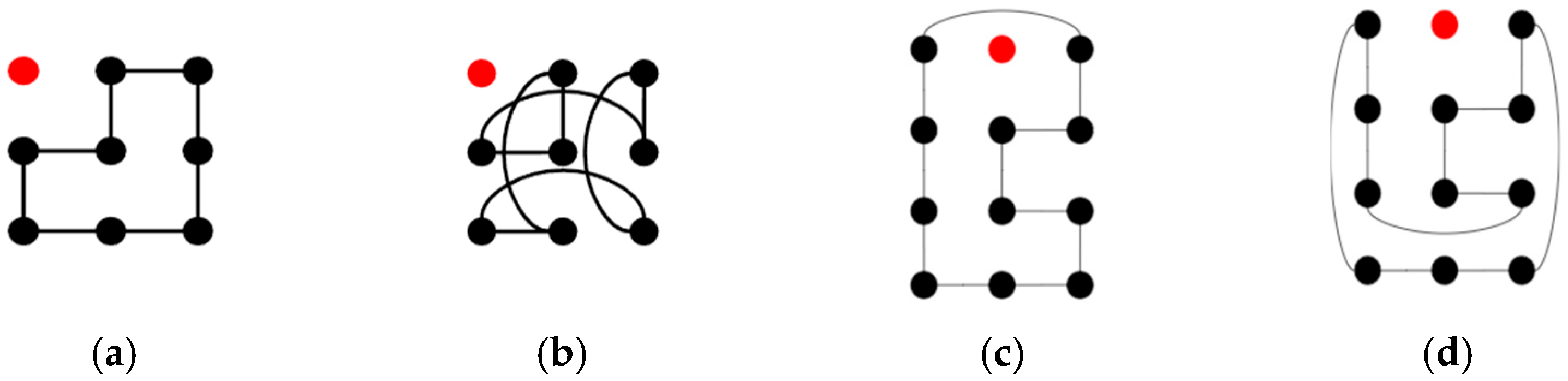
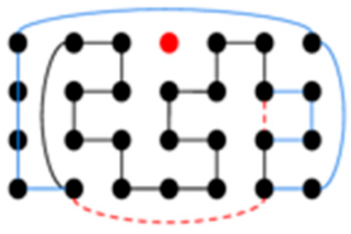
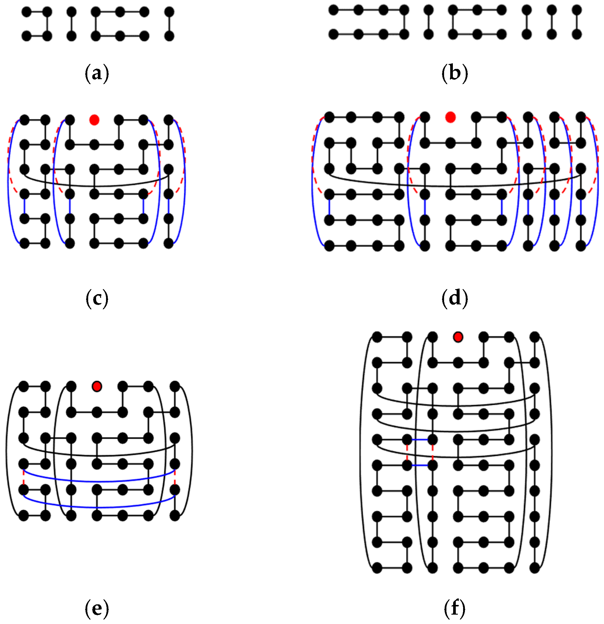
• Case 1.1. To construct a DBH with type (a): In the hypothesis, there is a DBH C₁ on T_m−2,4 with type (a) satisfying Claim 1. First, C₁ is put in the middle of T_m,4 with edges {(1, 0)(1, 3), (1, 3)(m − 2, 3), (m − 2, 0)(m − 2, 1), (m − 2, 1)(m − 2, 2)}, (m − 2, 2)(m − 2, 3)} in C₁. Then, remove {(1, 3)(m − 2, 3), (m − 2, 1)(m − 2, 2)} from C₁ and add {(m − 2, 1)(m − 1, 1), (m − 1, 1)(m − 1, 2), (m − 2, 2)(m − 1, 2), (m − 2, 3)(m − 1, 3), (m − 1, 0)(m − 1, 3), (0, 0)(m − 1, 0), (0, 0)(0, 1), (0, 1)(0, 2), (0, 2)(0, 3), (0, 3)(1, 3)} into C₁. After calculation, the operation requires adding four first-dimensional edges and four second-dimensional edges. We removed one first-dimensional edge and one second-dimensional edge and added five first-dimensional edges and five second-dimensional edges. Therefore, the constructed Hamiltonian cycle is of type (a), satisfies Claim 1, and is a DBH. Figure 6 shows an example of T_7,4 − F.

  Figure 6. The constructed DBH C₁ on T_7,4 − F.

  Figure 6. The constructed DBH C₁ on T_7,4 − F.

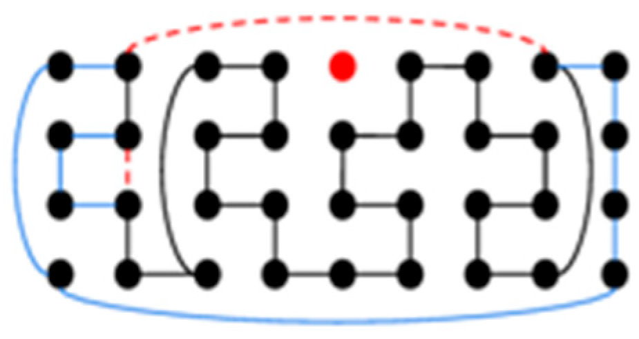
• Case 1.2. To construct a DBH with type (b): There is a DBH C₂ on T_m−2,4 with type (b) and that satisfies Claim 1. First, C₂ is put in the middle of T_m,4, with edge {(1, 1)(m − 2, 1)} in C₂. Then, {(1, 0)(1, 3), (1, 1)(m − 2, 1)} is removed to add {(0, 0)(1, 0), (0, 1)(1, 1), (0, 1)(0, 2), (0, 2)(m − 1, 2), (0, 3)(1, 3), (0, 0)(0, 3), (m − 2, 1)(m − 1, 1), (m − 1, 0)(m − 1, 1), (m − 1, 0)(m − 1, 3), (m − 1, 2)( m − 1, 3)}. After calculation, this operation requires adding four first-dimensional edges and four second-dimensional edges. We removed one first-dimensional and one second-dimensional edges and added five first-dimensional edges and five second-dimensional edges. Therefore, the constructed Hamiltonian cycle becomes type (b), satisfies Claim 1, and is a DBH. Figure 7 shows an example of the constructed C₂ on T_7,4 − F.

  Figure 7. Constructed DBH C₂ on T_7,4 − F.

  Figure 7. Constructed DBH C₂ on T_7,4 − F.

• Case 2. (m mod 4) = 1: There are also two DBHs on T_m,4 need to be constructed. Therefore, this case is divided into two parts and discussed separately depending on whether the constructed DBH is type (a) or (b).

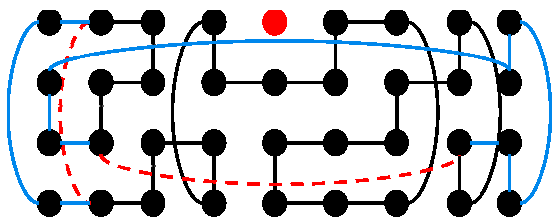
• Case 2.1. To construct a DBH with type (a), a DBH C₁ is used on T_m−2,4 with type (a) satisfying Claim 1. C₁ is similar to Figure 6 in this subcase. First, C₁ is put in the middle of T_m,4 with edges {(1, 0)(1, 1), (1, 1)(1, 2), (1, 2)(1, 3), (1, 0)(m − 2, 0), (m − 2, 0)(m − 2, 3)} in C₁. Then, remove {(1, 0)(m − 2, 0), (1, 1)(1, 2)} and add {(0, 0)(1, 0), (0, 1)(1, 1), (0, 1)(0, 2), (0, 2)(1, 2), (0, 0)(0, 3), (0, 3)(m − 1, 3), (m − 2, 0)(m − 1, 0), (m − 1, 0)(m − 1, 1), (m − 1, 1)(m − 1, 2), (m − 1, 2)(m − 1, 3)} into C₁. After calculation, this operation requires adding four first-dimensional edges and four second-dimensional edges. Similarly to case 1.1, we removed one first-dimensional edge and one second-dimensional edge and added five first-dimensional edges and five second-dimensional edges. Therefore, the constructed Hamiltonian cycle is of type (a), satisfies Claim 1, and is a DBH. Figure 8 shows an example of the constructed C₁ on T_9,4 − F.

  Figure 8. The constructed DBH C₁ of T_9,4 − F.

  Figure 8. The constructed DBH C₁ of T_9,4 − F.

• Case 2.2. To construct a DBH with type (b): There is a DBH C₂ on T_m−2,4 with type (b) satisfying Claim 1. C₂ is similar to Figure 7 in this subcase. First, C₂ is put in the middle of T_m,4 with edge {(1, 2)(m − 2, 2)} in C₂. Then, remove {(1, 0)(1, 3), (1, 2)(m − 2, 2)} and add {(0, 0)(1, 0), (0, 1)(0, 2), (0, 1)(m − 1, 1), (0, 2)(1, 2), (0, 3)(1, 3), (0, 0)(0, 3), (m − 2, 2)(m − 1, 2), (m − 1, 0)(m − 1, 1), (m − 1, 0)(m − 1, 3), (m − 1, 2)(m − 1, 3)}. Again, it can be determined that this operation requires adding four first-dimensional edges and four second-dimensional edges into C₂ to keep it dimension-balanced. We removed one first-dimensional edge and one second-dimensional edge and added five first-dimensional edges and five second-dimensional edges. Therefore, the constructed Hamiltonian cycle is of type (b) satisfying Claim 1 and a DBH. Figure 9 shows an example of the constructed C₂ on T_9,4 − F.

  Figure 9. The constructed DBH C₂ of T_9,4 − F.

  Figure 9. The constructed DBH C₂ of T_9,4 − F.

• Step 2. Two rows downward of T_m,n−2.

By Step 1, there exist two DBHs C₁ and C₂ with types (a) and (b), respectively, on T_m,4 − F. |E₁(C₁)| = |E₁(C₂)| = 2m − 1, and |E₂(C₁)| = |E₂(C₂)| = 2m. Then, if n > 4, let k = (n − 4)/2. We divided this step into two cases according to the number of (m mod 4) for discussion. Y_m is defined as the Cartesian product of C_m and P₂, called a prism graph, where P_n is a path with n vertices. The vertex set of Y_m is V(Y_m) = {(x, y) | 0 ≤ x ≤ m − 1; 0 ≤ y ≤ 1}, and the edge set E(Y_m) = {(x₁, y₁)(x₂, y₂) | x₁ = x₂ and |y₁ − y₂| = 1, or |x₁ − x₂| = (1 or m − 1) and y₁ = y₂}.

• Case 1. (m mod 4) = 1: There are two DBHs on T_m,n to be constructed. Therefore, this case is divided into two parts and discussed separately depending on whether the constructed DBH is type (a) or (b).

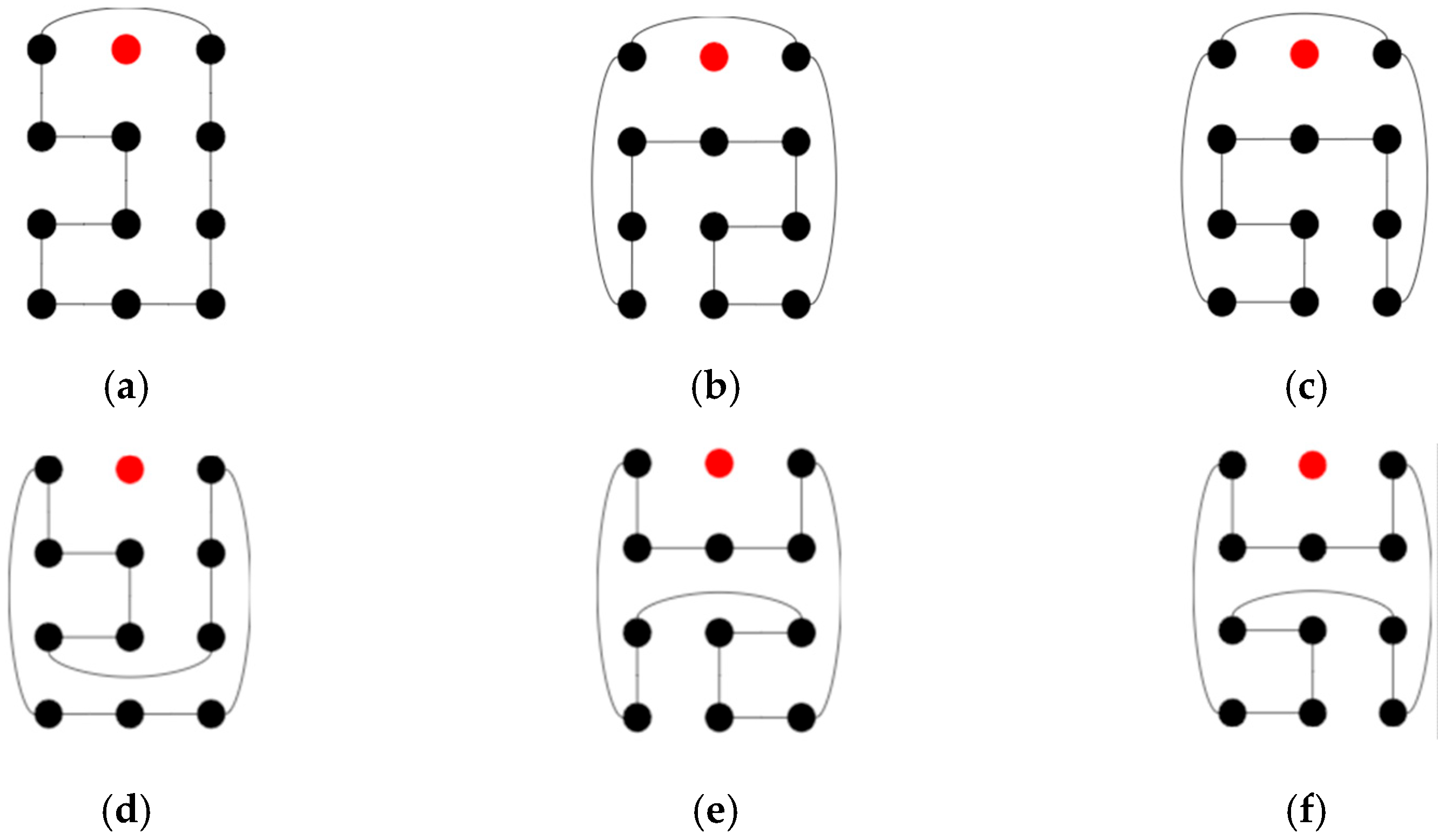
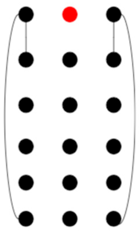
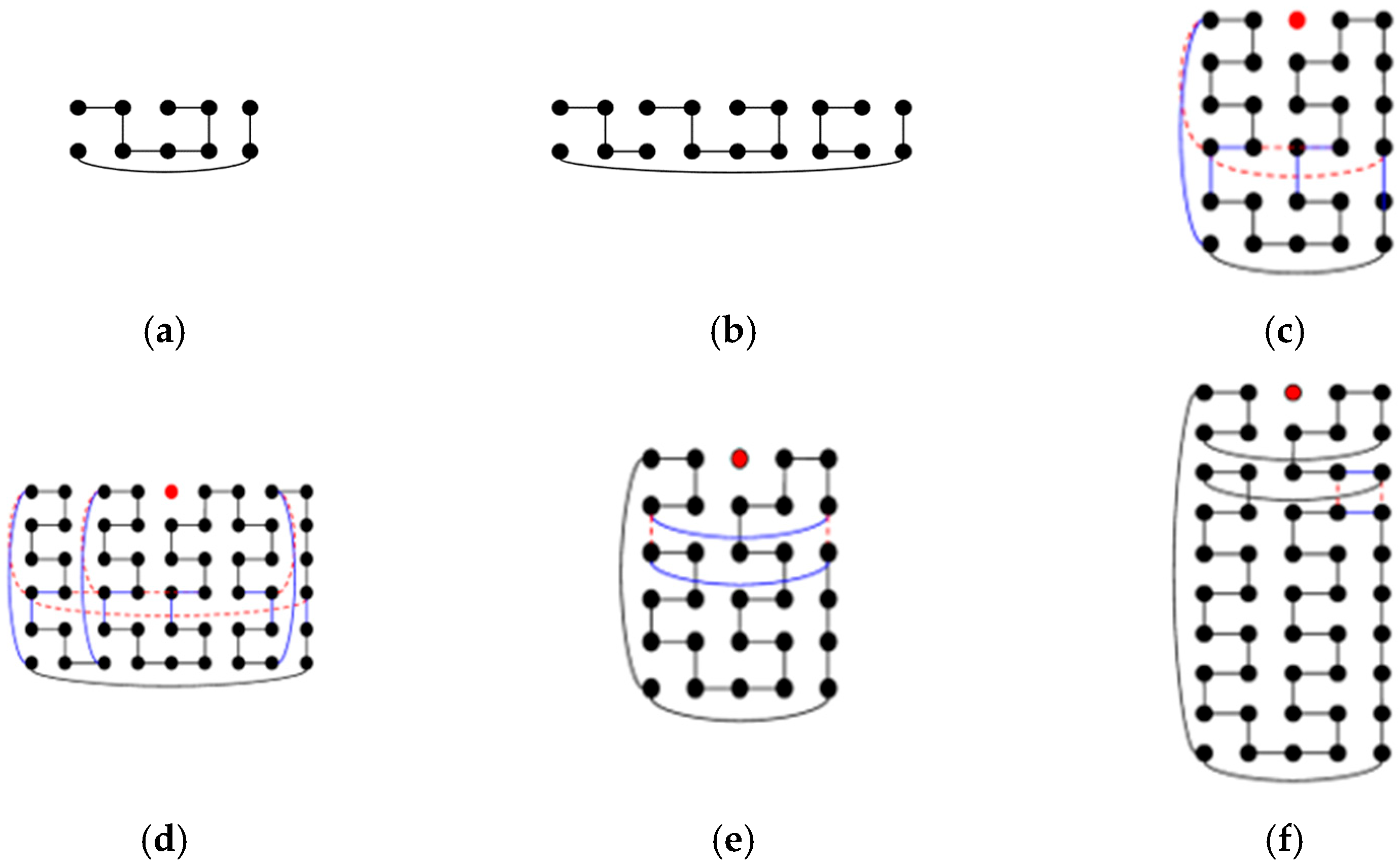
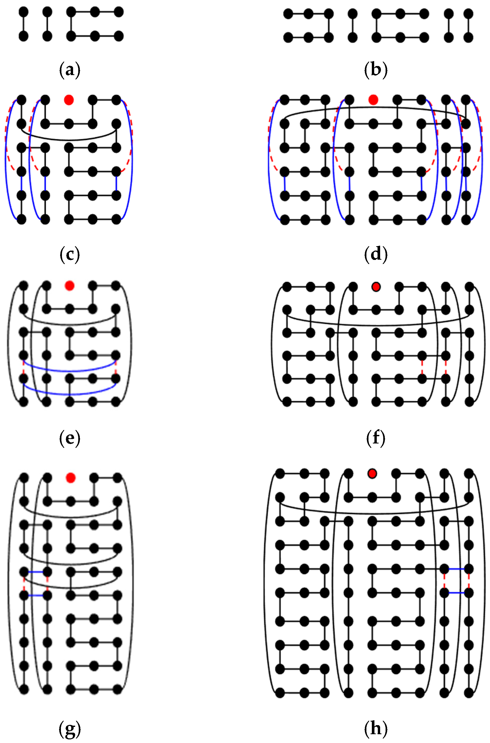
• Case 1.1. To construct a DBH with type (a): By Step 1, there is a DBH C₁ on T_m,4 with type (a). Copy the last two rows of C₁ to be a subgraph of Y_m named Z_m. Figure 10a,b show Z₅ and Z₉, respectively. Now, C₁ is put in the upper part of T_m,n, and k Z_ms in the lower part of T_m,n. Then, remove {(0, 3)(m − 1, 3)} ∪ {(2i, 0)(2i, 3), (2i + 1, 3 + 2j)(2i + 2, 3 + 2j) | 0 ≤ i < (m − 1)/4, 0 ≤ j < k} ∪ {(2i + 1, 0)(2i + 1, 3) | (m + 3)/4 ≤ i < (m − 1)/2} and add {(2i, 0)(2i, n − 1), (2i, 3 + 2j)(2i, 4 + 2j), (2i, 3 + 2j)(2i + 1, 3 + 2j) | 0 ≤ i < (m − 1)/4, 0 ≤ j < k } ∪ {(2i + 1, 0)(2i + 1, n − 1), (2i + 1, 3 + 2j)(2i + 1, 4 + 2j) | (m + 3)/4 ≤ i < (m − 1)/2, 0 ≤ j < k} ∪ {((m − 1)/2, 3 + 2j)((m − 1)/2, 4 + 2j), (m − 1, 3 + 2j)(m − 1, 4 + 2j) | 0 ≤ j < k}. Figure 10c,d show examples for T_5,6 − F, T_9,6 − F. After calculation, the generated Hamiltonian cycle C satisfies |E₁(C)| = |E₁(C₁)| + k(m − 1) = nm/2 − (k + 1) and |E₂(C)| = |E₁(C₁)| + k(m + 1) = nm/2 + k. We added k or k + 1 first-dimensional edges and removed k or k + 1 second-dimensional edges from C to form a type (a) DBH of T_m,n − F. There are two sub-steps according to the value of n that can solve this situation.

• Step 1.1.1. Let x = ⌊(n + 2)/8⌋ = ⌊(k + 3)/4⌋. Find x smallest i with {(0, i)(0, i + 1), (m − 1, i)(m − 1, i + 1)} ⊆ E(C). Then, remove (0, i)(0, i + 1), (m − 1, i)(m − 1, i + 1) and add (0, i)(m − 1, i), (0, i + 1)(m − 1, i + 1) to C. Figure 10e shows an example for T_5,6 − F. This step adds 2⌊(k + 3)/4⌋ first-dimensional edge and removes 2⌊(k + 3)/4⌋ second-dimensional edges from C.

• Step 1.1.2. Let x = ⌊(n − 2)/8⌋ = ⌊(k + 1)/4⌋. Find x smallest i with {(m − 2, i)(m − 2, i + 1), (m − 1, i)(m − 1, i + 1)} ⊆ E(C) and {(m − 2, i)(m − 1, i), (m − 2, i + 1)(m − 1, i + 1)} ⊄ E(C). Then, (m − 2, i)(m − 2, i + 1), (m − 1, i)(m − 1, i + 1) are removed, and (m − 2, i)(m − 1, i), (m − 2, i + 1)(m − 1, i + 1) are added into C. Figure 10f shows an example. This step adds 2⌊(k + 1)/4⌋ first-dimensional edges and removes 2⌊(k + 1)/4⌋ second-dimensional edges from C.

Note that 2⌊(k + 3)/4⌋ + 2⌊(k + 1)/4⌋ = k or k + 1. The created Hamiltonian cycle C is a DBH with type (a).

Figure 10. Examples for case 1.1 of Step 2 of Theorem 4. (a) Z₅, (b)Z₉, (c) a Hamiltonian cycle C on T_5,6 − F, (d) a Hamiltonian cycle C on T_9,6 − F, (e) the construct DBH of T_5,6 − F, (f) the construct DBH of T_5,10 − F.

Figure 10. Examples for case 1.1 of Step 2 of Theorem 4. (a) Z₅, (b)Z₉, (c) a Hamiltonian cycle C on T_5,6 − F, (d) a Hamiltonian cycle C on T_9,6 − F, (e) the construct DBH of T_5,6 − F, (f) the construct DBH of T_5,10 − F.

• Case 1.2. To construct a DBH with type (b): By Step 1, there is a DBH C₂ on T_m,4 with type (b). The last two rows of C₂ are copied to be a subgraph of Y_m named Z_m. Modify Z_m by adding edges {(0, 2i + 1)(0, 2i + 2) | 0 ≤ i ≤ (m − 9)/4} and deleting edges {(0, (m − 5)/2)(0, (m − 3)/2} ∪ {(0, 2i)(0, 2i + 1) | (m + 5)/4 ≤ i ≤ (m − 2)/2}. Figure 10a,b show Z₅ and Z₉, respectively. Then, C₂ is put in the upper part of T_m,n, and k Z_ms in the lower part of T_m,n. Then, for any 0 ≤ i ≤ m − 1, if edge (0, i)(3, i) is in C₂, this edge is removed, and edges {(0, i)(n − 1, i), (3 + 2j, i)(4 + 2j, i) | 0 ≤ j < k} are added to C₂ and k Z_ms to form a new Hamiltonian cycle C of T_m,n − F. Figure 11c,d show an example of T_5,6 − F and T_9,6 − F. Similarly to case 1.1, after calculation, the generated Hamiltonian cycle C satisfies |E₁(C)| = |E₁(C₁)| + k(m − 1) = nm/2 − (k + 1) and |E₂(C)| = |E₁(C₁)| + k(m + 1) = nm/2 + k. We added k or k + 1 first-dimensional edges and removed k or k + 1 second-dimensional edges from C to form a type (b) DBH of T_m,n − F. There are two sub-steps according to the value of n to solve this situation. m = 5 is a special case and needs to be discussed separately.

• Step 1.2.1. Let x = ⌊(n + 2)/8⌋ = ⌊(k + 3)/4⌋. For m = 5, find x smallest i with {(0, i)(0, i + 1), (m − 1, i)(m − 1, i + 1)} ⊆ E(C). Then, remove these two edges and add (0, i)(m − 1, i), (0, i + 1)(m − 1, i + 1) into C. Figure 11e shows an example. For m > 5, find x smallest i with {((m − 1)/2 + 2, i)((m − 1)/2 + 2, i + 1), ((m − 1)/2 + 3, i)((m − 1)/2 + 3, i + 1)} ⊆ E(C). Then, these two edges are removed, and ((m − 1)/2 + 2, i)((m − 1)/2 + 3, i), ((m − 1)/2 + 2, i + 1)((m − 1)/2 + 3, i + 1) are added to C. Figure 11f shows an example for T_9,6 − F.

• Step 1.2.2. Let x = ⌊(n − 2)/8⌋ = ⌊(k + 1)/4⌋. For m = 5, find the 2x edges (0, i)(0, i + 1), (1, i)(1, i + 1) such that (0, i)(1, i), (0, i + 1)(1, i + 1) ∉ E(C) (after performing Step 1.2.1). Then, (0, i)(0, i + 1), (1, i)(1, i + 1) are removed, and (0, i)(1, i), (0, i + 1)(1, i + 1) are added to C. Figure 11g shows an example for T_5,10 − F. For m > 5, find the 2x edges ((m − 1)/2 + 3, i)((m − 1)/2 + 3, i + 1), ((m − 1)/2 + 4, i)((m − 1)/2 + 4, i + 1) such that ((m − 1)/2 + 3, i)((m − 1)/2 + 4, i), ((m − 1)/2 + 3, i + 1)((m − 1)/2 + 4, i + 1) ∉ E(C) and i > 0. Then, ((m − 1)/2 + 3, i)((m − 1)/2 + 3, i + 1), ((m − 1)/2 + 4, i)((m − 1)/2 + 4, i + 1) are removed, and ((m − 1)/2 + 3, i)((m − 1)/2 + 4, i), ((m − 1)/2 + 3, i + 1)((m − 1)/2 + 4, i + 1) are added to C. Figure 11f shows an example for T_9,10 − F.

Note that 2⌊(k + 3)/4⌋ + 2⌊(k + 1)/4⌋ = k or k + 1, so the created Hamiltonian cycle C is a DBH with type (b).

Figure 11. Examples for case 1.2 of Step 2 of Theorem 4. (a) Z₅, (b)Z₉, (c) a Hamiltonian cycle C on T_5,6 − F, (d) a Hamiltonian cycle C on T_9,6 − F, (e) the construct DBH of T_5,6 − F, (f) the construct DBH of T_9,6 − F, (g) the construct DBH of T_5,10 − F, (h) the construct DBH of T_9,10 − F.

Figure 11. Examples for case 1.2 of Step 2 of Theorem 4. (a) Z₅, (b)Z₉, (c) a Hamiltonian cycle C on T_5,6 − F, (d) a Hamiltonian cycle C on T_9,6 − F, (e) the construct DBH of T_5,6 − F, (f) the construct DBH of T_9,6 − F, (g) the construct DBH of T_5,10 − F, (h) the construct DBH of T_9,10 − F.

• Case 2. (m mod 4) = 3: There are two DBHs on T_m,n constructed. Therefore, this case is divided into two parts and discussed separately depending on whether the constructed DBH is type (a) or type (b).

• Case 2.1. To construct a DBH with type (a): By Step 1, there is a DBH C₁ on T_m,n−2 with type (a). The last two rows of C₁ are copied to be a subgraph of Y_m named Z_m. Figure 12a,b show that Z₇ and Z₁₁. C₁ are put in the upper part of T_m,n, and k Z_ms in the lower part of T_m,n. Then, {(1 + 2i, 0)(1 + 2i, 3), (m − 1 − 2i, 0)(m − 1 − 2i, 3)| 0 ≤ i < (m − 3)/4} ∪ {(2i, 3 + 2j)(2i + 1, 3 + 2j)| 0 ≤ i < (m + 1)/4, 0 ≤ j < k} are removed, and {(1 + 2i, 0)(1 + 2i, n − 1), (m − 1 − 2i, 0)(m − 1 − 2i, n − 1), (1 + 2i, 3 + 2j)(2 + 2i, 3 + 2j), (1 + 2i, 3 + 2j)(1 + 2i, 4 + 2j), (m − 1 − 2i, 3 + 2j)(m − 1 − 2i, 4 + 2j)| 0 ≤ i < (m − 3)/4, 0 ≤ j < k } ∪ {((m − 1)/2, 3 + 2j)((m − 1)/2, 4 + 2j), (0, 3 + 2j)(0, 4 + 2j) | 0 ≤ j < k} are added. Figure 12c,d show T_7,6 − F and T_11,6 − F. After calculation, the generated Hamiltonian cycle C will satisfy |E₁(C)| = |E₁(C₁)| + k(m − 1) = nm/2 − (k + 1) and |E₂(C)| = |E₂(C₁)| + k(m + 1) = nm/2 + k. We added k or k + 1 first-dimensional edges and removed k or k + 1 second-dimensional edges from C to form a type (a) DBH of T_m,n − F. There are two sub-steps according to the value of n that can solve this situation.

• Step 2.1.1. Let x = ⌊(n + 2)/8⌋ = ⌊(k + 3)/4⌋. First, {(0, 4i + 1)(0, 4i + 2), (m − 1, 4i + 1)(m − 1, 4i + 2) | 0 ≤ i < x} are removed from C, and then {(0, 4i + 1)(m − 1, 4i + 1), (0, 4i + 2)(m − 1, 4i + 2) | 0 ≤ i < x} are added to C. Figure 12e shows an example for T_7,6 − F. In total, 2⌊(k + 3)/4⌋ first-dimensional edges are added to remove 2⌊(k + 3)/4⌋ second-dimensional edges from C.

• Step 2.1.2. Let x = ⌊(n − 2)/8⌋ = ⌊(k + 1)/4⌋. Then, {(0, 4i + 3)(0, 4i + 4), (1, 4i + 3)(1, 4i + 4) | 0 ≤ i < x} are removed from C, and {(0, 4i + 3)(1, 4i + 3), (0, 4i + 4)(1, 4i + 4) | 0 ≤ i < x} are added to C. Figure 12f shows an example of T_7,10 − F. This step adds 2⌊(k + 1)/4⌋ first-dimensional edges and removes 2⌊(k + 1)/4⌋ second-dimensional edges from C.

Note that 2⌊(k + 3)/4⌋ + 2⌊(k + 1)/4⌋ = k or k + 1, so the created Hamiltonian cycle C is a DBH with type (a).

Figure 12. Examples for case 2.1 of Step 2 of Theorem 4. (a) Z₇, (b)Z₁₁, (c) a Hamiltonian cycle C on T_7,6 − F, (d) a Hamiltonian cycle C on T_11,6 − F, (e) the construct DBH of T_7,6 − F, (f) the construct DBH of T_7,10 − F.

Figure 12. Examples for case 2.1 of Step 2 of Theorem 4. (a) Z₇, (b)Z₁₁, (c) a Hamiltonian cycle C on T_7,6 − F, (d) a Hamiltonian cycle C on T_11,6 − F, (e) the construct DBH of T_7,6 − F, (f) the construct DBH of T_7,10 − F.

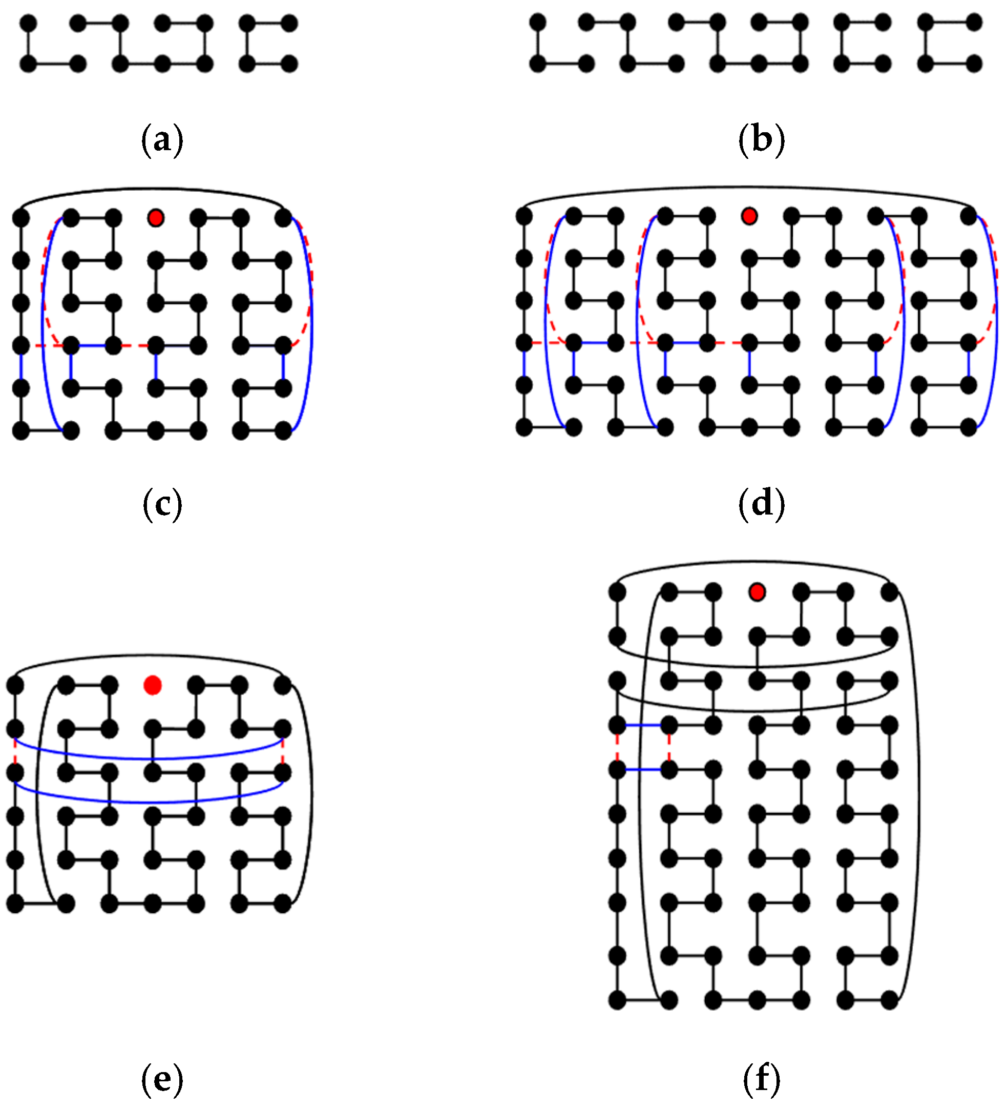
• Case 2.2. To construct a DBH with type (b): By Step 1, there is a DBH C₂ on T_m,4 with type (b). The last two rows of C₂ are copied to be a subgraph of Y_m named Z_m. Z_m is modified by adding edges {(0, 2i)(0, 2i + 1) | 0 ≤ i ≤ (m − 7)/4} and deleting edges {(0, (m − 5)/2)(0, (m − 3)/2} ∪ {(0, 2i)(0, 2i + 1) | (m + 5)/4 ≤ i ≤ (m − 3)/2}. Figure 13a,b show Z₇ and Z₁₁, respectively. Then, C₂ is put in the upper part of T_m,n, and k Z_ms in the lower part of T_m,n. Then, for any 0 ≤ i ≤ m − 1, if edge (0, i)(3, i) is in C₂, then this edge is removed to add edges {(0, i)(n − 1, i), (3 + 2j, i)(4 + 2j, i) | 0 ≤ j < k} into C₂ and k Z_ms to form a new Hamiltonian cycle C of T_m,n − F. Figure 13c,d show examples of T_7,6 − F and T_11,6 − F. Similarly to case 2.1, after calculation, the generated Hamiltonian cycle C satisfies |E₁(C)| = |E₁(C₁)| + k(m − 1) = nm/2 − (k + 1) and |E₂(C)| = |E₁(C₁)| + k(m + 1) = nm/2 + k. We added k or k + 1 first-dimensional edges and removed k or k + 1 second-dimensional edges from C to form a type (b) DBH of T_m,n − F. There are two sub-steps according to the value of n to solve this problem.

• Step 2.2.1. Let x = ⌊(n + 2)/8⌋ = ⌊(k + 3)/4⌋. Find the x smallest i with {(0, i)(0, i + 1), (m − 1, i)(m − 1, i + 1)} ⊆ E(C). Then, these two edges are removed, and (0, i)(m − 1, i), (0, i + 1)(m − 1, i + 1) are added to C. Figure 13e shows an example of T_7,6 − F.

• Step 2.2.2. Let x = ⌊(n − 2)/8⌋ = ⌊(k + 1)/4⌋. Find the x edge pairs ((m − 1)/2 − 2, i)((m − 1)/2 − 2, i + 1), ((m − 1)/2 − 1, i)((m − 1)/2 − 1, i + 1) such that ((m − 1)/2 − 2, i)((m − 1)/2 − 1, i), ((m − 1)/2 − 2, i + 1)((m − 1)/2 − 1, i + 1) ∉ E(C), and i > 3. Then, ((m − 1)/2 − 2, i)((m − 1)/2 − 2, i + 1), ((m − 1)/2 − 1, i)((m − 1)/2 − 1, i + 1) are removed, and ((m − 1)/2 − 2, i)((m − 1)/2 − 1, i), ((m − 1)/2 − 2, i + 1)((m − 1)/2 − 1, i + 1) are added to C. Figure 13f shows an example of T_7,10 − F.

Again, because of 2⌊(k + 3)/4⌋ + 2⌊(k + 1)/4⌋ = k or k + 1, so the created Hamiltonian cycle C is a DBH with type (b). □

Figure 13. Examples for case 2.2 of Step 2 of Theorem 4. (a) Z₇, (b)Z₁₁, (c) a Hamiltonian cycle C on T_7,6 − F, (d) a Hamiltonian cycle C on T_11,6 − F, (e) the construct DBH of T_7,6 − F, (f) the construct DBH of T_7,10 − F.

Figure 13. Examples for case 2.2 of Step 2 of Theorem 4. (a) Z₇, (b)Z₁₁, (c) a Hamiltonian cycle C on T_7,6 − F, (d) a Hamiltonian cycle C on T_11,6 − F, (e) the construct DBH of T_7,6 − F, (f) the construct DBH of T_7,10 − F.

4. Conclusions

We discussed whether T_m,n is a two-fault DBH or not, focusing on the one-node one-edge DBH problem. For any m and n, the conclusions of this study are summarized in Table 1. When both m and n are even, T_m,n is not a one-node one-edge DBH; and when one of m and n is odd (>3) and the other is even, T_m,n is a one-node one-edge DBH. It is proven that T_3,n is not the one-node one-edge DBH for any n ≥ 5. In the subsequent study where m and n are both odd, it is also proven that T_5,5 is not the one-node one-edge DBH. Due to space limitations, this part of the proof is omitted in this article. Finally, we provide a conjecture that when both m and n are odd and at least one is >5, T_m,n is not the one-node one-edge DBH.

Conjecture 1.

There is no DBH on T_m,n − F when m and n ≥ 5, where F is a set of any one node and one edge.

Table 1. Summary of one-node one-edge DBHs on T_m,n.

	m = 3	m Is Odd (>3)	m = 4	m Is Even (>4)
n = 3	Yes (Thm 3)	No (Thm 3)	Yes (Thm 3)	No (Thm 3)
n is odd (>3)	No (Thm 3)	No (Conjecture 1)	Yes (Thm 4)
n = 4	Yes (Thm 3)	Yes (Thm 4)	No (Thm 1)
n is even (>4)	No (Thm 3)

Table 1. Summary of one-node one-edge DBHs on T_m,n.

	m = 3	m Is Odd (>3)	m = 4	m Is Even (>4)
n = 3	Yes (Thm 3)	No (Thm 3)	Yes (Thm 3)	No (Thm 3)
n is odd (>3)	No (Thm 3)	No (Conjecture 1)	Yes (Thm 4)
n = 4	Yes (Thm 3)	Yes (Thm 4)	No (Thm 1)
n is even (>4)	No (Thm 3)

References

- Dimakopoulos, V.V.; Palios, L.; Poulakidas, A.S. On the Hamiltonicity of the Cartesian Product. Inform. Process. Lett. 2005, 96, 49–53. [Google Scholar] [CrossRef]
- Kim, H.-C.; Park, J.-H. Fault Hamiltonicity of Two-Dimensional Torus Networks. In Proceedings of the Workshop on Algorithms and Computation WAAC’00, Tokyo, Japan, 21–22 July 2000; pp. 110–117. [Google Scholar]
- Du, Z.-Z.; Xu, J.-M. A Note on Cycle Embedding in Hypercubes with Faulty Vertices. Inf. Process. Lett. 2011, 111, 557–560. [Google Scholar] [CrossRef]
- Wang, H.-R. The Balanced Hamiltonian Cycle Problem. Master’s Thesis, Department of Computer Science and Information Engineering, National Chi-Nan University, Nantou, Taiwan, 2011. [Google Scholar]
- Peng, W.-F.; Juan, J.S.-T. The Balanced Hamiltonian Cycle on the Toroidal Mesh Graphs. World Academy of Science, Engineering and Technology, Open Science Index 65. Int. J. Comput. Inf. Eng. 2012, 6, 674–680. [Google Scholar]
- Wu, R.-Y.; Lai, Z.-Y.; Juan, J.S.-T. The Weakly Dimension-Balanced Hamiltonian. In Proceedings of the International Conference on Parallel and Distributed Processing Techniques and Applications (PDPTA), Las Vegas, NV, USA, 30 July–2 August 2018; pp. 178–182. [Google Scholar]
- Juan, J.S.-T.; Lai, Z.-Y. The Weakly Dimension-Balanced Pancyclicity on Toroidal Mesh Graph Tm,n When Both m and n Are Odd. In Lecture Notes in Computer Science; Springer: Cham, Switzerland, 2021; Volume 13025, pp. 437–448. [Google Scholar]
- Hsu, H.-C.; Chiang, L.-C.; Tan, J.J.; Hsu, L.-H. Fault hamiltonicity of augmented cubes. Parallel Comput. 2005, 31, 131–145. [Google Scholar] [CrossRef]
- Cheng, C.-W.; Lee, C.-W.; Hsieh, S.-Y. Conditional Edge-Fault Hamiltonicity of Cartesian Product Graphs. IEEE Trans. Parallel Distrib. Syst. 2013, 24, 1951–1960. [Google Scholar] [CrossRef]
- Abdallah, M.; Cheng, E. Fault-Tolerant Hamiltonian Connectivity of 2-Tree-Generated Networks. Theor. Comput. 2022, 907, 62–81. [Google Scholar] [CrossRef]
- Juan, J.S.-T.; Ciou, H.-C.; Lin, M.-J. The One-Fault Dimension-Balanced Hamiltonian Problem on Toroidal Mesh Graph. Symmetry 2005, 17, 93. [Google Scholar] [CrossRef]
- Xu, J. Theory and Application of Graphs; Kluwer Academic Publishers: Norwell, MA, USA, 2003. [Google Scholar]
Disclaimer/Publisher’s Note: The statements, opinions and data contained in all publications are solely those of the individual author(s) and contributor(s) and not of MDPI and/or the editor(s). MDPI and/or the editor(s) disclaim responsibility for any injury to people or property resulting from any ideas, methods, instructions or products referred to in the content. |
© 2025 by the authors. Licensee MDPI, Basel, Switzerland. This article is an open access article distributed under the terms and conditions of the Creative Commons Attribution (CC BY) license (https://creativecommons.org/licenses/by/4.0/).
Share and Cite
Chang, Y.Y.-C.; Juan, J.S.-T. One-Node One-Edge Dimension-Balanced Hamiltonian Problem on Toroidal Mesh Graph. Eng. Proc. 2025, 89, 17. https://doi.org/10.3390/engproc2025089017
Chang YY-C, Juan JS-T. One-Node One-Edge Dimension-Balanced Hamiltonian Problem on Toroidal Mesh Graph. Engineering Proceedings. 2025; 89(1):17. https://doi.org/10.3390/engproc2025089017
Chicago/Turabian StyleChang, Yancy Yu-Chen, and Justie Su-Tzu Juan. 2025. "One-Node One-Edge Dimension-Balanced Hamiltonian Problem on Toroidal Mesh Graph" Engineering Proceedings 89, no. 1: 17. https://doi.org/10.3390/engproc2025089017
APA StyleChang, Y. Y.-C., & Juan, J. S.-T. (2025). One-Node One-Edge Dimension-Balanced Hamiltonian Problem on Toroidal Mesh Graph. Engineering Proceedings, 89(1), 17. https://doi.org/10.3390/engproc2025089017