Low-Cost SDR for GNSS Interference Mitigation Using Spatial Diversity Techniques ^†

Abstract

This paper addresses the feasibility of implementing spatial diversity techniques to mitigate interference signals using low-cost GNSS receivers. Global Navigation Satellite Systems (GNSSs) remain at the core of navigation technologies and obtaining precise and robust positioning solutions in harsh scenarios becomes essential for the proper functioning of modern applications. Furthermore, this challenge is even more complex when mass-market receivers are addressed, since the previous requirements must be achieved while maintaining low-cost architectures. A promising solution is to use beamforming techniques, which exploit the spatial domain to achieve enhanced reliability and robustness. In this paper, the potential of beamforming in mass-market receivers is analyzed by implementing two interference mitigation techniques and using a five-channel low-cost software defined radio (SDR), KrakenSDR. The results show that the algorithms implemented are able to mitigate strong interference signals, allowing the GNSS receiver to compute an accurate positioning solution.

1. Introduction

Despite the emergence of new positioning approaches experienced in recent years, Global Navigation Satellite Systems (GNSSs) are still the standard and reference technology when implementing navigation and positioning solutions. Today, the number of infrastructures that rely on these systems to properly function is substantial and, with new use cases continuously appearing in the civil domain, the requirements in terms of accuracy and reliability of the position, velocity, and time (PVT) solutions are intensified.

The aforementioned demands are not new for certain GNSS sectors, where high accuracy positioning was already a need in the past, but offering precision and robustness in low-cost GNSS receivers aimed at the mass-market is still a challenge. The tendency towards miniaturization, along with the cost and complexity constraints characteristic of these devices, severely restrict the performance of GNSS mass-market receivers. This is particularly accentuated in hostile scenarios, where the coexistence of a high number of technologies tends to degrade the performance of the services.

Under these circumstances, it is common to find undesired contributions impinging on the receiver along with the GNSS signal, causing interference, which pose a major threat when it occurs inside the bandwidth used by the receiver. When this occurs, the interference cannot be filtered out in the frequency domain, and its presence will inevitably affect the performance. In cases where these contributions are too powerful, the front-end of the receiver is saturated, resulting in an erroneous digital conversion of the received signal that does not allow the receiver to operate at all [1]. In less extreme cases, i.e., where the front-end of the receiver can still function properly, the problem arises during the despreading process, where the power of the interference will be spanned across the bandwidth and lead to noisier measurements that result in inaccuracies in the final positioning solution.

Measures should therefore be taken to ensure a proper provision of the service even under these circumstances. In this scope, exploiting spatial diversity has proved to be a very powerful approach [2,3]. Originally, the use of multi-antenna solutions in the GNSS domain was linked to the defense sector, where controlled radiation pattern antennas (CRPA) are typically used to filter out undesired contributions based on their direction of arrival (DoA) [4,5,6,7]. However, the technological advances in recent years have enabled the exploitation of the spatial domain through digital beamforming techniques and applications such as 5G, Internet of Things (IoT), and the most recent IEEE 802.11 standards have greatly benefited from them [8,9,10,11].

A crucial aspect in the deployment of said multi-antenna techniques is to maintain a separation between consecutive elements of half the wavelength to ensure an undistorted spatial response, and so services using higher frequencies bands take advantage of this. An inter-element spacing of half-wavelength in the GNSS domain requires a distance of $~96$ mm and $~128$ mm between antennas, for the L1/E1 and L5/E5 bands, respectively. These values are much larger than those observed in the 5G field, where the millimeter wave nature allows a minimum separation of the sensors of $\sim 5\mathrm{mm}$, and so moving these multi-antenna configurations into mass-market GNSS receivers comes with several challenges.

However, the technological advances experienced in this domain, along with the projections for the near future in terms of miniaturization and lower cost elements, position spatial diversity in smaller GNSS receivers as a great solution to tackle the concerns aroused by undesired contributions [12,13]. In this work, the suitability of multi-antenna configurations in said devices is analyzed through experimental studies, where two low complexity spatial diversity techniques are implemented and evaluated using a multi-channel software-defined radio (SDR) representative of mass-market devices, the KrakenSDR, together with a Spirent set-up capable of simulating a GPS constellation affected by interference.

2. Fundamentals of Array Processing

2.1. Signal Model

Let us consider an antenna array formed by L elements receiving one contribution directly from the satellite constellation, i.e., the line-of-sight signal (LOSS), along with I undesired signals, i.e., the interference. The combination of the signals perceived by the antennas can be arranged into an $L\times 1$ vector $\mathit{x}\left[n\right]$, resulting in the complex baseband signal depicted in Equation (1).

$$\mathit{x}\left[n\right]=\mathit{a}({\theta }_0)s\left[n\right]+\sum _{j=1}^I\mathit{a}\left({\theta }_j\right)i_j\left[n\right]+\mathit{n}\left[n\right]$$

(1)

From the expression in Equation (1), $s\left[n\right]$ depicts the desired LOSS, $i_j\left[n\right]$ the j-th interference, and $\mathit{n}\left[n\right]$ the noise experienced at each channel. The term $\mathit{a}\left(\theta \right)\in {\mathbb{C}}^{L\times 1}$ describes the spatial signature of the contribution arriving from direction $\theta$ as perceived by the L elements in the array, where the subscript ₀ is used to refer to the LOSS and _j to the different interference.

For the sake of simplicity, under the assumption that a single interference is impinging the array along with the desired GNSS signals, the signal model becomes the one presented in Equation (2).

$$\mathit{x}\left[n\right]=\mathit{a}\left({\theta }_0\right)s\left[n\right]+\mathit{a}\left({\theta }_j\right)i_j\left[n\right]+\mathit{n}\left[n\right]$$

(2)

Lastly, mind that the previous notation describes the signal before the despreading process, i.e., before the correlation with the local code is performed, and thus the GNSS signal, although present in the expressions above, is not visible for the receiver at this stage, since it is well-buried below the noise floor. Following this reasoning, and under the assumption that the power of the interference is noticeable, one can benefit from this property to simplify the expression in Equation (2) into the one in Equation (3), which will be very useful when applying the beamforming techniques presented.

$$\mathit{x}\left[n\right]=\mathit{a}\left({\theta }_0\right)s\left[n\right]+\mathit{a}\left({\theta }_j\right)i_j\left[n\right]+\mathit{n}\left[n\right]\approx \mathit{a}\left({\theta }_j\right)i_j\left[n\right]+\mathit{n}\left[n\right]$$

(3)

2.2. The Beamforming Principle

The term beamforming describes the process of linearly combining the samples received from each of the antennas in the receiver to obtain, at the output of the array, a single sample. How said linear combination is performed will define the purpose of the beamformer, which is normally, as in the case of this work, to filter out any type of interference while maintaining the desired contribution. This is achieved through the application of a set of spatial coefficients or weights, $\mathit{w}\in {\mathbb{C}}^{L\times 1}$, to the spatial samples presented in Equation (1). The result is a single sample at the output of the beamformer, $y\left[n\right]$, as it is expressed in Equation (4).

$$y\left[n\right]={\mathit{w}}^H\mathit{x}\left[n\right]$$

(4)

Hence, the essence of the problem is determining the weights in $\mathit{w}$ that should be applied according to a certain optimization criterion, and this is where the beamforming techniques come into play, as they will be the ones dictating the values of the coefficients.

3. Exploiting Spatial Diversity for Interference Mitigation

Given that before the despreading process, the GNSS signal remains buried below the noise floor, there is little to no information that can be acquired from it. In certain cases, one can have information about its DoA, relying on external services that provide the satellite ephemerides and with knowledge of the receiver’s orientation or by applying specific techniques for direction finding [14,15]. However, in the case of GNSS, direction finding entails despreading the signal and working at post-correlation once it is visible, which, as previously stated, is not always possible when an interference is present.

Considering these limitations and the goal of a low-complexity scheme at the receiver, this work analyses two blind beamforming techniques. The term “blind” is used to state that these algorithms do not need any prior knowledge or additional information to compute the weights, and only the incoming samples ($\mathit{x}\left[n\right]$) are evaluated by to produce the set of coefficients.

3.1. Power Inversion Beamformer

The Power Inversion beamformer (PI) aims to minimize the power at the output of the antenna array while keeping one of the channels, namely the reference element, undisturbed [16]. This entails computing the weights minimizing the total output power, ${\left|{\mathit{w}}^H\mathit{x}\left[n\right]\right|}^2$, but keeping the coefficient associated with the reference element equal to one, which leads to the optimization problem stated in Equation (5).

$${\mathit{w}}_{\mathrm{P}\mathrm{I}}=\underset{\mathit{w}}{\min }{\mathit{w}}^H\mathit{x}\left[n\right]{\mathit{x}}^{\mathit{H}}\left[n\right]\mathit{w}\mathrm{subject}\mathrm{to}{\mathit{w}}^H\underset{\mathsf{\delta }}{\underbrace{\left[\begin{array}{c}1\\ 1\\ ⋮\\ 1\end{array}\right]}}=1$$

(5)

Note from the expression above that $\mathit{x}\left[n\right]{\mathit{x}}^{\mathit{H}}\left[n\right]$ is the instantaneous autocorrelation matrix, denoted by ${\mathit{R}}_{\mathit{x}}\left[n\right]$. After processing N consecutive samples, one can estimate the averaged autocorrelation matrix ${\mathit{R}}_{\mathit{x}}$ as ${\mathit{R}}_{\mathit{x}}={\displaystyle \frac{1}{N}}\sum _{n=1}^N\mathit{x}\left[n\right]{\mathit{x}}^{\mathit{H}}\left[n\right]$, and use it to obtain a more robust formulation.

The problem statement presented in Equation (5) is easily solved by Lagrange multipliers, leading to the optimum solution of the weights to be the one presented in Equation (6).

$${\mathit{w}}_{\mathrm{P}\mathrm{I}}={\displaystyle \frac{{\mathit{R}}_{\mathit{x}}^{-1}\mathsf{\delta }}{{{\mathit{\delta }}^{\mathit{H}}\mathit{R}}_{\mathit{x}}^{-1}\mathit{\delta }}}$$

(6)

See that in order to obtain the previous expression, which provides the coefficients of the beamformer, no more information than that received by the antenna array is used, and thus this technique can be rightly called blind.

3.2. Prewhitening Beamformer

The fact that GNSS signals are buried below the noise floor when they first arrive at the receiver can be exploited to obtain an interference free signal at the output of the beamformer. This approach, known as Prewhitening beamformer (PREW), is the one followed in the technique presented in [17], where the autocorrelation matrix is decomposed and manipulated to obtain an interference-free subspace in which to project the incoming samples. Due to the uncorrelation between the interference and the LOSS, the projection of the samples contained in $\mathit{x}\left[n\right]$ onto this interference free subspace results in output samples where the undesired contributions have been suppressed.

The essence of this algorithm lies, therefore, in finding a projection matrix that allows the receiver to eradicate the interference. To achieve this, the first step involves decomposing the autocorrelation matrix into its eigenvectors and eigenvalues, considering the signal model defined in Equation (3), where the presence of the LOSS can be omitted since it is imperceptible. This simplified but effective version of the decomposition is depicted in Equation (7).

$${\mathit{R}}_{\mathit{x}}\approx \mathit{U}{\mathsf{\Lambda }\mathit{U}}^H={\mathit{U}}_{\mathit{i}}\left({\mathsf{\Lambda }}_{\mathit{i}}+{\sigma }_n^2\mathit{I}\right){{\mathit{U}}_{\mathit{i}}}^H+{{\sigma }_n^2\mathit{U}}_n{{\mathit{U}}_n}^H$$

(7)

From the previous expression, ${\mathit{U}}_{\mathit{i}}\in {\mathbb{C}}^{L\times I}$ is a matrix containing the eigenvectors of the interference subspace that are associated with the eigenvalues ${\mathsf{\lambda }}_i$ enclosed in the diagonal matrix ${\mathsf{\Lambda }}_{\mathit{i}}$. Similarly, ${\mathit{U}}_n\in {\mathbb{C}}^{L\times \left(L-I\right)}$ holds the eigenvectors that span the noise subspace, and ${\sigma }_n^2$ represents the noise power.

With the expression in Equation (7), a whitening matrix $\mathit{W}$ can be found through the Mahalanobis whitening procedure. Applying said matrix to the incoming signal allows the decorrelation of the contributions present in $\mathit{x}\left[n\right]$, ensuring the orthogonality between the interference and the LOSS. Therefore, the resulting whitening matrix $\mathit{W}$ has the form presented in Equation (8).

$$\mathit{W}={\mathit{R}}_{\mathit{x}}^{-{\displaystyle \frac{1}{2}}}={\mathit{U}}_{\mathit{i}}{\left({\mathsf{\Lambda }}_{\mathit{i}}+{\sigma }_n^2\mathit{I}\right)}^{-{\displaystyle \frac{1}{2}}}{\mathit{U}}_{\mathit{i}}^H+{\displaystyle \frac{1}{\sqrt{{\sigma }_n^2}}}{\mathit{U}}_n{\mathit{U}}_n^H$$

(8)

It can be fairly presumed that the power of the interference will be much higher than that of the noise, so the eigenvalues of the interference will be larger than the noise power, i.e., ${\mathsf{\lambda }}_i\gg {\sigma }_n^2$; thus, the whitening matrix can be approximated as stated in Equation (9).

$$\mathit{W}={{\mathit{R}}_{\mathit{x}}}^{-{\displaystyle \frac{1}{2}}}\approx {\displaystyle \frac{1}{\sqrt{{\sigma }_n^2}}}{\mathit{U}}_n{{\mathit{U}}_n}^H$$

(9)

Note now that the resulting whitening matrix $W\approx {\displaystyle \raisebox{1ex}{$1$}\!\left/ \!\raisebox{-1ex}{${\sigma }_n$}\right.}{\mathit{U}}_n{{\mathit{U}}_n}^H$ is the projection matrix onto the interference free subspace, and so when applied to $\mathit{x}\left[n\right]$, as depicted in Equation (10), the result will be samples free of the undesired contributions, denoted by $\tilde{\mathit{x}}\left[n\right]$.

$$\tilde{\mathit{x}}\left[\mathit{n}\right]=\mathit{W}\mathit{x}\left[n\right]$$

(10)

Lastly, once the received signal is clean from interference, the weights can be easily selected as the eigenvector associated with the largest eigenvalue of the new autocorrelation matrix obtained from the modified samples, i.e., ${\tilde{\mathit{R}}}_{\mathit{x}}={\displaystyle \frac{1}{N}}\sum _{n=1}^N\tilde{\mathit{x}}\left[n\right]{\tilde{\mathit{x}}}^H\left[n\right]$, obtaining the final coefficients as depicted in Equation (11), where $\mathcal{P}\left\{·\right\}$ represents the operator that retrieves the eigenvector associated with the largest eigenvalue.

$${\mathit{w}}_{PREW}=\mathcal{P}\left\{{\tilde{\mathit{R}}}_{\mathit{x}}\right\}$$

(11)

Again, the weights presented in Equation (11) have been obtained with no more information than that extracted from the received signal, resulting in another blind approach.

4. Experimental Analysis

The two techniques introduced in the previous section have been implemented and tested using an architecture representative of low-cost mass-market GNSS receivers, with the purpose of showing and proving the efficacy of spatial diversity techniques in this type of devices. In this section, the scheme used for the experiments conducted is detailed, together with a thorough analysis of the results obtained.

4.1. Architecture and Experiment Description

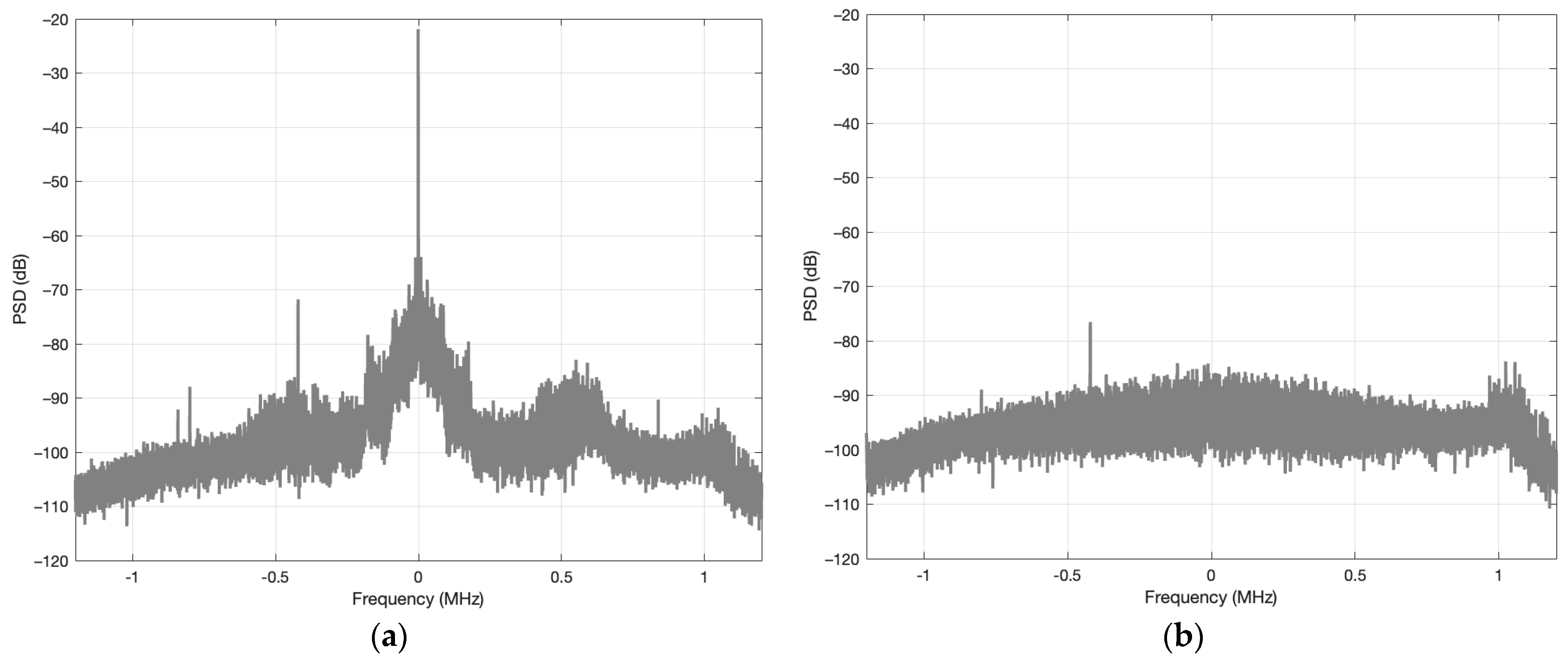
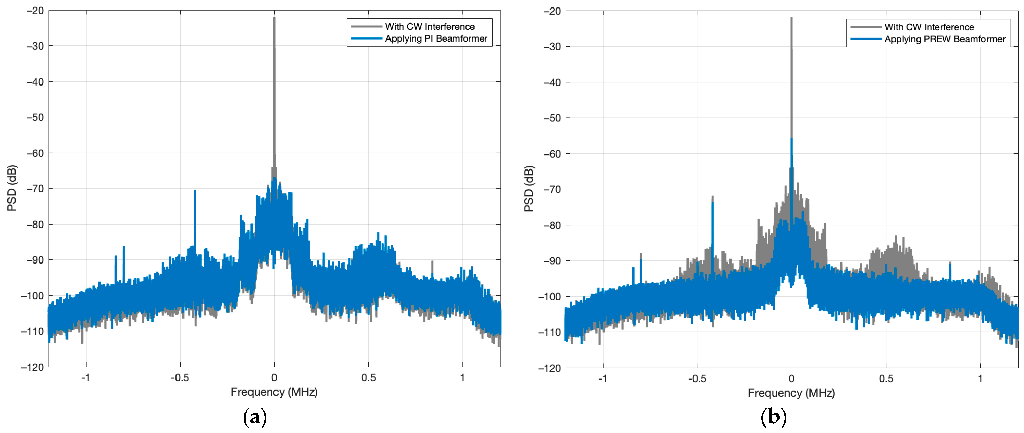
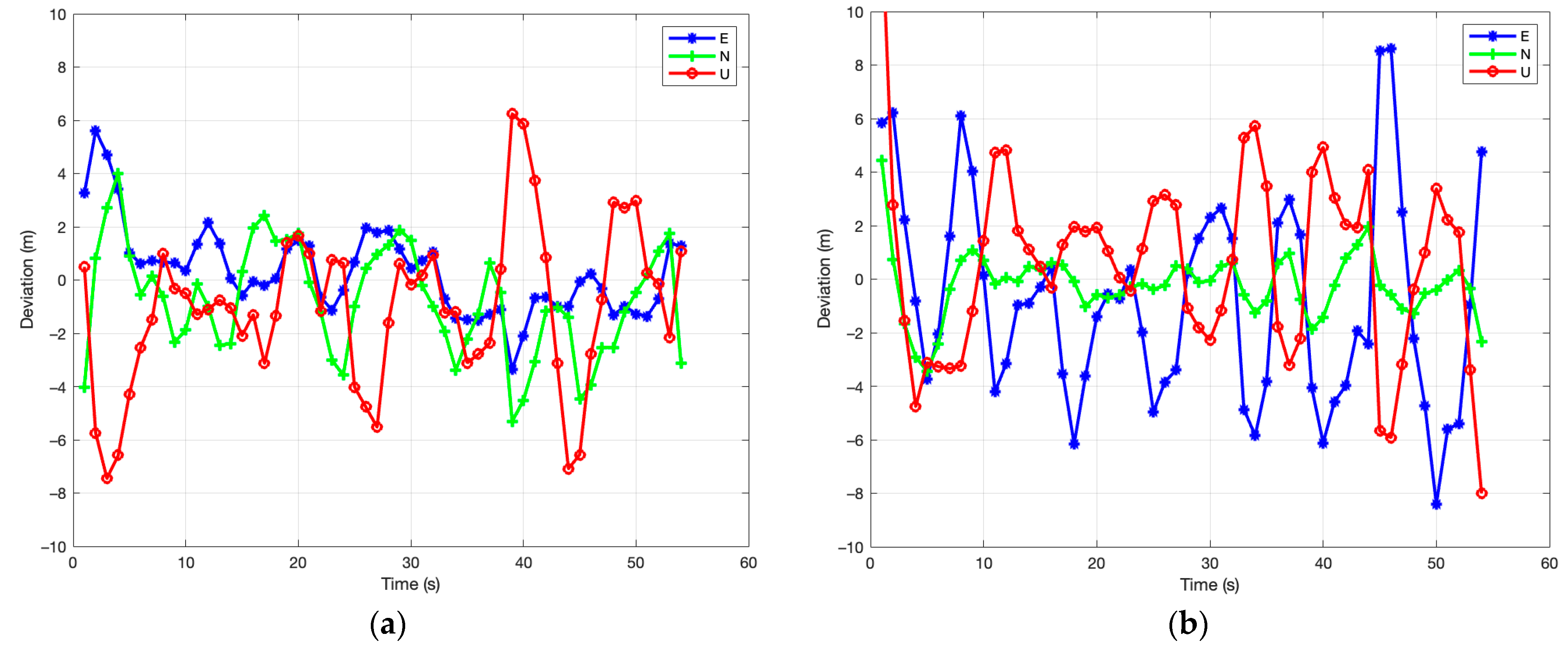
As briefly introduced at the beginning of this paper, a custom-made Spirent set-up with four output channels was employed to simulate a GPS L1 constellation affected by a continuous wave (CW) interference, which was placed at the central frequency of the L1 band, i.e., 1575.42 MHz, with a power level 70 dB greater than that of the GPS signals.

On the receiver side, the KrakenSDR, a low-cost SDR with capabilities to process up to five channels, was used. In this study, the four outputs generated by Spirent were captured and sampled using this SDR with a sampling frequency of 2.4 MHz, mimicking a uniform linear array (ULA) configuration respecting the inter-element separation of half-wavelength of the L1 band. To increase the levels of the received signals, four low noise amplifiers (LNAs) had to be connected at its input ports to guarantee an appropriate processing of the samples.

After the simulation, each channel of the KrakenSDR results in a data file containing the signal received with its corresponding phase offset due to the ULA configuration. These four data files were the input for the beamforming module, where the PI and the PREW algorithms were applied independently. The resulting signal obtained after the application of each algorithm was introduced into the FGI-GSRx-v1.0.0 software receiver, which allowed the processing of the output samples, presenting the final positioning solution along with certain valuable metrics for the analysis, as it is the carrier-to-noise density ratio (C/N0) and the deviation from the real location of the user [18]. For the processing of the GPS signals, an integration time of 15 ms was used, along with the Least Squares Estimator (LSE) to solve the navigation equations and obtain the positioning solution, using only those satellites with an elevation above 5° and a C/N0 level higher than 30 dB-Hz.

4.2. Results

With the aim of acquiring a reference on the performance of the receiver in regular conditions, this is, without any external impairment that may hinder its operation, the first experiment conducted consisted in processing the Spirent-simulated GPS signals when no interference was present. The results obtained in this case are presented in Figure 1, in terms of C/N0 in graph (a) and in terms of deviation from the true position in each of the East (E), North (N), and Up (U) in (b).

It can be appreciated from Figure 1a that under favorable conditions, nine GPS satellites are visible—satellites 2, 4, 5, 10, 12, 24, 29, 30 and 31—all achieving C/N0 levels around 45 dB-Hz for the entire simulation. This leads to the promising accuracy in the positioning solution observed in Figure 1b, where the error in all three ENU coordinates lies below 2 m.

However, the positive performance observed in this setting will inevitably deteriorate when an undesired contribution appears in the scenario. The consequence of a CW interference with the characteristics presented at the beginning of this section is exhibited in Figure 2, where the power spectral density (PSD) of the received signal in the presence of the CW interference is shown together with the PSD when only GPS contributions imping the array, in plots (a) and (b), respectively.

The impact that the CW has on the receiver can be observed though the PSD of Figure 2a, where the contribution of the interference is clearly seen at the central frequency. Comparing this result with the one in Figure 2b, which is essentially the PSD of the noise since the GPS signals are still buried, one can perceive a large difference in terms of power. The 70 dB increase observed in the presence of the CW interference completely saturates the receiver, making it impossible to acquire the GPS signals and thus impeding the computation of the positioning solution.

It is in this case where beamforming plays a key role. The deployment of spatial diversity techniques such as the ones introduced in the previous section can significantly improve the performance of the receiver, effectively mitigating the interference and allowing the processing of the GPS signals. When the PI and PREW beamforming techniques are implemented and applied to the received samples, the resulting power level of the CW contribution is greatly decreased, since the algorithms are capable of spatially filtering out the undesired component. This can be observed in Figure 3, where the PSD at the output of the PI and PREW beamformers is presented, in Figure 3a for the PI, and in Figure 3b for the PREW. In both cases, the spectrum of the received signal affected by the interference before applying the techniques is plotted along, with the purpose of facilitating the comparison.

The PSD obtained in the two techniques presented clearly shows that the power of the interference has been largely diminished, almost 50 dB for the PI beamformer in Figure 3a and around 35 dB for the PREW beamformer in Figure 3b. This meaningful attenuation in the power of the interference achieved exploiting spatial diversity allows the GNSS receiver to properly process the GPS signals, thus making it able to compute the positioning solution. In Figure 4, the deviation from the true position of the user is depicted, in Figure 4a for the case of the PI beamformer and in Figure 4b for the PREW.

The fact that applying these two low-complexity beamforming techniques, where no additional information is needed to compute the coefficients of the spatial filter, allows the receiver to acquire and track the GPS signals is, in itself, a great achievement. However, not only do these simple algorithms enable the operation of the receiver but they also provide very positive results in terms of positioning error, as is shown in both plots of Figure 4. Note that in both cases, the deviation from the true coordinates is of 10 m at worst, which is a remarkably promising performance for devices with these characteristics, i.e., low-cost mass-market receivers.

Lastly,

Table 1. Summary of the relevant metrics obtained in each experiment.

Technique	Sat. Availability	Avg. C/N0 [dB-Hz]	3D RMS [m]
Only GPS signals	9/9	46.164	1.216
PI beamformer	8/9	36.697	4.154
PREW beamformer	7/9	39.308	5.487

offers a summary covering the most remarkable aspects of the receiver performance, where the 3-Dimensional Root-Mean-Square (3D RMS) error has been used to combine the individual E, N, and U deviations and offer an overall result.

It is clear from the information presented in Table 1 that the PI beamformer slightly outperforms the PREW beamformer, offering a higher satellite availability and, therefore, a smaller 3D RMS error, as one additional satellite is used with the PI algorithm to compute the position. Nevertheless, despite this minor difference between the two techniques, the results presented in this work confirm that the deployment of multiple antennas in mass-market GNSS devices with restricted capabilities is indeed feasible, and it can significantly improve the performance of the receiver in hostile scenarios, where undesired contributions are a great threat.

5. Conclusions

The present paper evaluated the feasibility of exploiting spatial diversity in GNSS mass-market receivers, whose performance in adverse conditions is largely affected by their low-cost components. To solve these deficiencies, the use of two low-complexity multi-antenna techniques was analyzed and proved to be effective when counteracting the effects of undesired contributions, which remain a serious threat in the GNSS domain. The two techniques under study, the PI and PREW beamformers, were implemented using a representative mass-market SDR, the KrakenSDR, whose four channels were configured forming a ULA. This device, together with the Spirent simulator, allowed us to analyze the behavior of the GNSS receiver implementing the two beforementioned techniques when a CW interference is present. The results obtained prove the efficiency of multi-antenna algorithms in this domain, particularized for the cases of the PI and PREW beamformers, showing that the negative impact of external contributions can be effectively mitigated by deploying undemanding beamforming techniques suitable for low-cost devices.

References

1. Hegarty, C.; Kaplan, E. Understanding GPS Principles and Applications, 2nd ed.; Artech: Norwood, MA, USA, 2005. [Google Scholar]
2. Lam, N.H.B. Angle of Arrival Estimation for Low Power and Long Range Communication Networks; University of Antwerp: Antwerp, Belgium, 2021. [Google Scholar]
3. BniLam, N.; Principe, F.; Crosta, P. Large Array Antenna Aperture for GNSS Applications. IEEE Trans. Aerosp. Electron. Syst. 2024, 60, 675–684. [Google Scholar] [CrossRef]
4. Volakis, J.L.; O’Brien, A.J.; Chen, C.-C. Small and Adaptive Antennas and Arrays for GNSS Applications. Proc. IEEE 2016, 104, 1221–1232. [Google Scholar] [CrossRef]
5. Williams, D.; Clark, S.; Cook, J.; Corcoran, P.; Spaulding, S. Four-Element Adaptive Array Evaluation for United States Navy Airborne Applications. In Proceedings of the 13th International Technical Meeting of the Satellite Division of The Institute of Navigation (ION GPS 2000), Salt Lake City, UT, USA, 19–22 September 2000; pp. 2523–2532. [Google Scholar]
6. Berz, G.; Barret, P.; Disselkoen, B.; Richard, M.; Bleeker, O.; Rocchia, V.; Jacolot, F.; Bigham, T. Interference Localization using a Controlled Radiation Pattern Antenna (CRPA). In Proceedings of the 29th International Technical Meeting of the Satellite Division of The Institute of Navigation (ION GNSS+ 2016), Portland, OR, USA, 12–16 September 2016; pp. 3053–3062. [Google Scholar]
7. Vegni, C.; Neri, A. GNSS Interference: Effects and Solutions. In Proceedings of the ION 2015 Pacific PNT Meeting, Honolulu, HI, USA, 20–23 April 2015; pp. 454–469. [Google Scholar]
8. Vook, F.W.; Ghosh, A.; Thomas, T.A. MIMO and Beamforming Solutions for 5G Technology. In Proceedings of the 2014 IEEE MTT-S International Microwave Symposium (IMS2014), Tampa, FL, USA, 1–6 June 2014; pp. 1–4. [Google Scholar] [CrossRef]
9. Larsson, E.G.; Edfors, O.; Tufvesson, F.; Marzetta, T.L. Massive MIMO for next generation wireless systems. IEEE Commun. Mag. 2014, 52, 186–195. [Google Scholar] [CrossRef]
10. Deng, C.; Fang, X.; Han, X.; Wang, X.; Yan, L.; He, R.; Long, Y.; Guo, Y. IEEE 802.11be Wi-Fi 7: New Challenges and Opportunities. IEEE Commun. Surv. Tutor. 2020, 22, 2136–2166. [Google Scholar] [CrossRef]
11. BniLam, N.; Ergeerts, G.; Subotic, D.; Steckel, J.; Weyn, M. Adaptive probabilistic model using angle of arrival estimation for IoT indoor localization. In Proceedings of the 2017 International Conference on Indoor Positioning and Indoor Navigation (IPIN), Sapporo, Japan, 18–21 September 2017; pp. 1–7. [Google Scholar] [CrossRef]
12. Egea-Roca, D.; Arizabaleta-Diez, M.; Pany, T.; Antreich, F.; López-Salcedo, J.A.; Paonni, M.; Seco-Granados, G. GNSS User Technology: State-of-the-Art and Future Trends. IEEE Access 2022, 10, 39939–39968. [Google Scholar] [CrossRef]
13. Swindlehurst, A.; Jeffs, B.; Seco-Granados, G.; Li, J. Chapter 20. Applications of Array Signal Processing. Acad. Press Libr. Signal Process. 2014, 3, 859–953. [Google Scholar] [CrossRef]
14. Roy, R.; Kailath, T. ESPRIT-estimation of signal parameters via rotational invariance techniques. IEEE Trans. Acoust. Speech Signal Process. 1989, 37, 984–995. [Google Scholar] [CrossRef]
15. Stoica, P.; Sharman, K.C. Maximum likelihood methods for direction-of-arrival estimation. IEEE Trans. Acoust. Speech Signal Process. 1990, 38, 1132–1143. [Google Scholar] [CrossRef]
16. Compton, R.T. The Power-Inversion Adaptive Array: Concept and Performance. IEEE Trans. Aerosp. Electron. Syst. 1979, AES-15, 803–814. [Google Scholar] [CrossRef]
17. Sgammini, M.; Antreich, F.; Kurz, L.; Meurer, M.; Noll, T. Blind Adaptive Beamformer Based on Orthogonal Projections for GNSS. In Proceedings of the 25th International Technical Meeting of The Satellite Division of the Institute of Navigation (ION GNSS 2012), Nashville, TN, USA, 17–21 September 2012. [Google Scholar]
18. Borre, K.; Fernández-Hernández, I.; López-Salcedo, J.A.; Bhuiyan, M.Z.H. (Eds.) GNSS Software Receivers; Cambridge University Press: Cambridge, UK, 2022. [Google Scholar] [CrossRef]
Figure 1. Results when only GPS L1 signals are present: (a) in terms of C/N0; (b) in terms of deviation from the true position.
Engproc 88 00007 g001
Figure 2. PSD of the received signal (a) in the presence of a CW interference; (b) when only GPS L1 signals arrive.
Engproc 88 00007 g002
Figure 3. PSD of the received signal before and after applying (a) PI beamformer; (b) PREW beamformer.
Engproc 88 00007 g003
Figure 4. Error in the positioning solution after applying (a) PI beamformer; (b) PREW beamformer.
Engproc 88 00007 g004