Global Ionospheric Corrections: Enhancing High-Accuracy Positioning ^†

Abstract

Electrically charged particles present in this layer of the Earth’s atmosphere can alter radio waves, such as those from GPS, Galileo, or BeiDou, resulting in non-estimated errors with respect to the available navigation models for the end user. For most positioning algorithms based in sequential filters, this effect is translated into a slow convergence towards a solution around the decimeter error level. If we consider that the ionosphere’s effect varies based on the user’s location and solar activity due to the atmosphere particle composition, it becomes clear that a global accurate model, valid across wide areas accounting for different seasons and timespans, is, at the very least, quite challenging. The focus of this paper is the demonstration of a global ionosphere model designed to improve the positioning accuracy of the end user through the estimation of ionospheric corrections to the broadcasted navigation message. Mathematically, this method is based on a spherical harmonic expansion model. This approach has the advantage of reducing the dependency from a highly densified station network where the ionosphere delay must be constantly estimated in dozens of locations, in favor of a simplified model that barely needs to be adjusted with a limited set of real-time data (around 40 stations). In this case, GMV’s global station network was used, which comprises geodetic-grade receivers tracking the signal in open-sky locations around the globe. The global ionospheric model is configured to process signals from GPS and Galileo constellations. To evaluate the performances of this model on the final user position estimation, several precise point positioning (PPP) solutions were computed at different locations. The results were compared with PPP solutions calculated without ionospheric corrections at the same stations. The goal of this paper is to show the significant performance improvement observed with the implementation of the global model.

1. Introduction

The significance of high-accuracy services has grown over time, driven by the rising demand in markets such as autonomous car navigation and precision agriculture. Precise point positioning (PPP) is a high-accuracy technique that relies only on orbit and clock corrections. While PPP typically achieves accuracies in the range of centimeters, one of its drawbacks has been the slow time required to achieve a fully converged solution [1]. However, it has been demonstrated that this challenge can be mitigated by developing precise models of the ionosphere and using them as a correction for PPP-RTK.

Extending from around 75 km to 2000 km above sea level, the ionosphere plays a fundamental role in global communications and navigation systems. This layer of the terrestrial atmosphere contains molecules and electrically charged particles, predominantly ions and free electrons, which arise from the interaction of solar radiation with the upper atmosphere and the incidence of charged particles. This ionized medium can reflect and modify electromagnetic signals. The electron density or total electron content (TEC) of the ionosphere varies with height and is influenced by factors such as the geographic location of the receiver, the time of day, and the intensity of the solar activity [2]. Due to this reason, estimating the impact of this layer on GNSS electromagnetic signals is quite challenging.

Mitigating the effects of ionospheric disturbances is crucial for accurate positioning. Various correction techniques are employed to counteract these influences. One method is the employment of spherical harmonic models, which represent the ionospheric delay of GNSS signals as a series of mathematical functions. These models offer a comprehensive yet computationally intensive approach to correction. Grid-based correction methods divide the service area (regional, wide-area, or global) into a grid. Each point of the grid gives the user the ionospheric delay on that point to be interpolated in the user position. This method balances accuracy with computational efficiency. Additionally, slant ionospheric delays estimated over different GNSS stations can be sent to users together with the station positions to allow the user to interpolate the ionospheric delay on its position. This method requires a larger number of stations, computational cost, and bandwidth.

This paper focuses on the construction of a global ionosphere model through spherical harmonic expansion techniques, employing a limited number of dual-frequency receivers. Section 2 provides an explanation of the methodology used for model calculation, as well as insights into its application in PPP-RTK. The evaluation of the computed model under various convergence scenarios is presented in Section 3.

2. Methodology

2.1. Generation of Global Ionospheric Corrections

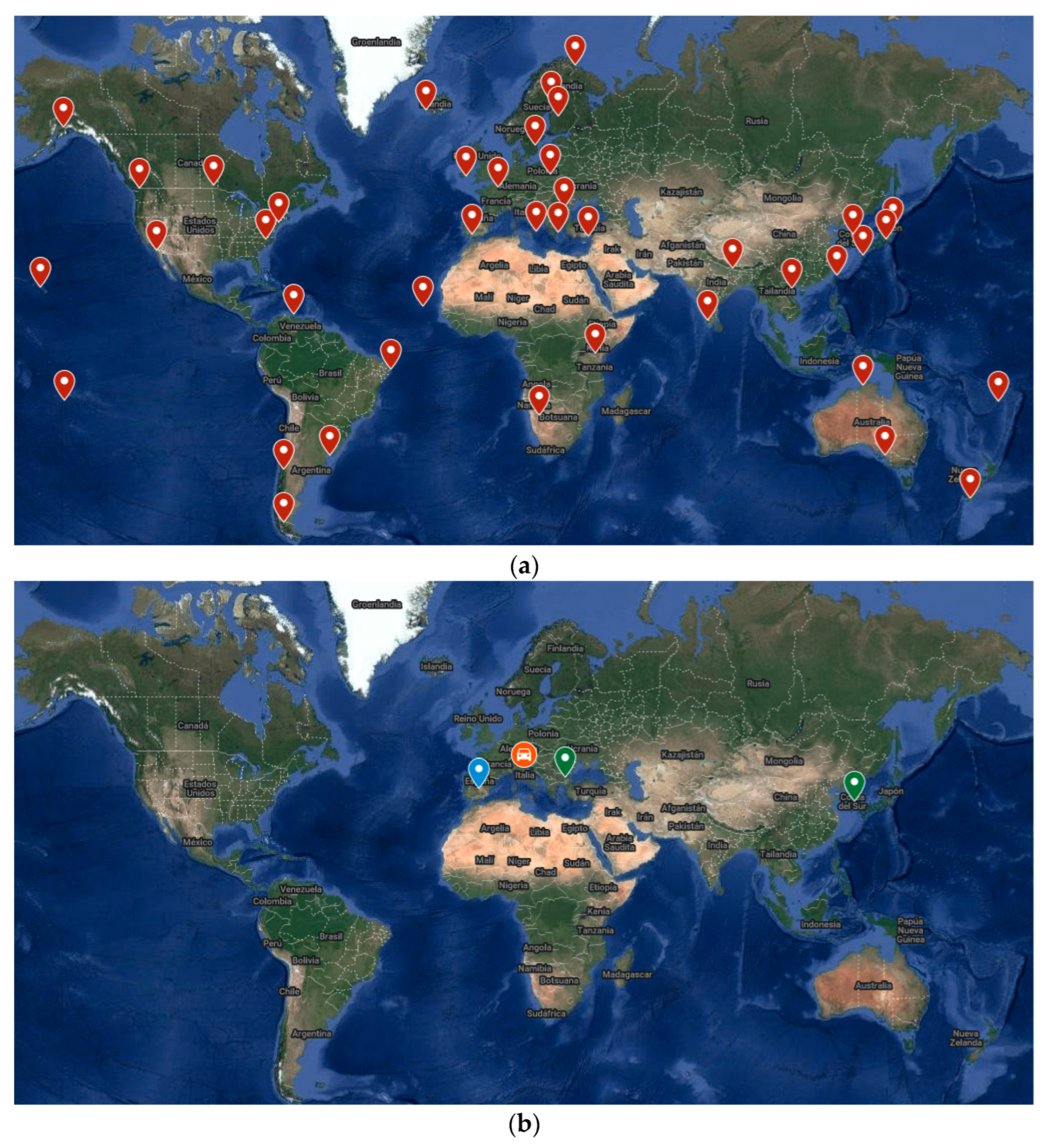
In this paper, 41 GNSS stations from the GMV’s GGRN (Global GNSS Reference Network) private network were used to calculate a global ionosphere model [3]. This network was strategically planned to ensure an evenly distributed placement of its stations, as illustrated in Figure 1. Equipped with geodetic receivers, these stations enabled the computation of PPP using Ionosphere-free and wide-lane combinations. Given the known positions of the stations, the result of PPP computation provides estimated slant ionospheric delay values for each line of sight in the network. These data will be used as input for the model calculation. However, these slant values include unknown biases per satellite and per station, as shown in Equation (1), that must be estimated:

$$\mathrm{I}=\mathrm{I}’+{\mathrm{B}}_{\mathrm{S}\mathrm{A}\mathrm{T}}+{\mathrm{B}}_{\mathrm{G}\mathrm{S}\mathrm{S}}$$

(1)

where I is the estimated slant ionospheric delay in the pierce-point, I’ is the real slant ionospheric delay, ${\mathrm{B}}_{\mathrm{S}\mathrm{A}\mathrm{T}}$ is the bias per satellite, and ${\mathrm{B}}_{\mathrm{G}\mathrm{S}\mathrm{S}}$ denotes the bias per station.

As mentioned earlier, the ionosphere is located between 75 km and 2000 km in height. For the development of the model, it was assumed that the majority of the total electron content was concentrated within a thin layer approximately 450 km above ground level. After determining this altitude and knowing the satellite position, the vertical equivalent of slant ionospheric delay value for each line of sight could be calculated using the modified mapping function [4], as shown in Equation (2):

$${\mathrm{I}}_{\mathrm{V}}={\displaystyle \frac{\mathrm{I}’}{\mathrm{M}\left(\mathrm{z}\right)}}$$

(2)

where ${\mathrm{I}}_{\mathrm{V}}$ is the vertical slant ionospheric delay in the pierce-point and M(z) denotes the mapping function.

To generate the global ionospheric corrections, we applied the spherical harmonic expansion technique shown in Equation (3):

$${\mathrm{I}}_{\mathrm{V}}={\sum }_{n=0}^{{\mathrm{n}}_{\mathrm{m}\mathrm{a}\mathrm{x}}}{\sum }_{\mathrm{m}=0}^{\mathrm{n}}\widetilde{{\mathrm{P}}_{\mathrm{n}\mathrm{m}}}(\mathrm{s}\mathrm{i}\mathrm{n}\mathsf{\beta })·({\mathrm{a}}_{\mathrm{n}\mathrm{m}}\mathrm{c}\mathrm{o}\mathrm{s}(\mathrm{m}\mathrm{s})+{\mathrm{b}}_{\mathrm{n}\mathrm{m}}\mathrm{s}\mathrm{i}\mathrm{n}(\mathrm{m}\mathrm{s})),$$

(3)

where n is the degree of spherical harmonic expansion, ${\mathrm{n}}_{\mathrm{m}\mathrm{a}\mathrm{x}}$ denotes the maximum degree, m is the order (m: {0…n}), $\widetilde{{\mathrm{P}}_{\mathrm{n}\mathrm{m}}}$ is the normalized associated Legendre function, ${\mathrm{a}}_{\mathrm{n}\mathrm{m}}$ and ${\mathrm{b}}_{\mathrm{n}\mathrm{m}}$ are the coefficients of the spherical harmonics, β denotes the geocentric latitude, and s is the sun-fixed longitude of the pierce-point [5].

Considering the spherical harmonic expansion and substituting the vertical slant value for the definition of the slant ionosphere delay, the reconstruction of the measurement for each line of sight is defined in Equation (4) as follows:

$$\mathrm{I}-\mathrm{M}(\mathrm{z})·\sum _{\mathrm{n}=0}^{{\mathrm{n}}_{\mathrm{m}\mathrm{a}\mathrm{x}}}\sum _{\mathrm{m}=0}^{\mathrm{n}}\widetilde{{\mathrm{P}}_{\mathrm{n}\mathrm{m}}}\left(\mathrm{s}\mathrm{i}\mathrm{n}\mathsf{\beta }\right)·\left({\mathrm{a}}_{\mathrm{n}\mathrm{m}}\mathrm{c}\mathrm{o}\mathrm{s}\left(\mathrm{m}\mathrm{s}\right)+{\mathrm{b}}_{\mathrm{n}\mathrm{m}}\mathrm{s}\mathrm{i}\mathrm{n}\left(\mathrm{m}\mathrm{s}\right)\right)-{\mathrm{B}}_{\mathrm{S}\mathrm{A}\mathrm{T}}-{\mathrm{B}}_{\mathrm{G}\mathrm{S}\mathrm{S}}=0$$

(4)

To estimate unknown parameters, a linear quadratic estimation or Kalman filter was utilized. The input measurements consisted of the I values for each line of sight. The parameters estimated at every epoch were the coefficients of the spherical harmonic expansion, along with biases per satellite and per station. A zero average constraint was applied in the bias per satellite estimation.

2.2. Use of Global Ionospheric Corrections

After estimating the coefficients, the model became applicable for evaluation at any point on the surface with known coordinates, employing the spherical harmonic expansion outlined in Equation (3). It is noteworthy that the determination of values for n and m should match those used in coefficient calculation. Once the vertical slant ionospheric delay at the pierce-point is obtained, ionosphere correction can be achieved using the mapping function, as shown in Equation (2).

2.3. Performance Analysis

The initial point of the performance analysis will be the generation of the input slant ionospheric delay values for each line of sight. As previously mentioned, data from the GMV network was utilized to compute a PPP-RTK solution for each station. GPS and Galileo constellations are taken into account in PPP-RTK calculations, processing GPS G1C, G2P and Galileo E1C, E5B signals.

After calculating these input values, spherical harmonic coefficients were estimated with a maximum expansion degree of 10. This degree was selected based on previous studies, which have demonstrated that it yields optimal results, providing a good balance between accuracy and model complexity without excessively increasing the computational load.

To evaluate the computed model, open sky static PPP-RTK scenarios were analyzed in several locations (Europe and South Korea) with and without global ionosphere corrections over a one-week period. Reconvergences of 30 min time span were launched every 5 min since the beginning of the scenario. Two of the chosen monitoring stations were part of the international GNSS service (IGS) GPS reference stations [6]. The third scenario used a F9P U-blox receiver with a geodetic antenna located in Madrid [7]. These monitoring receivers are represented in Figure 1 by green and blue points, respectively.

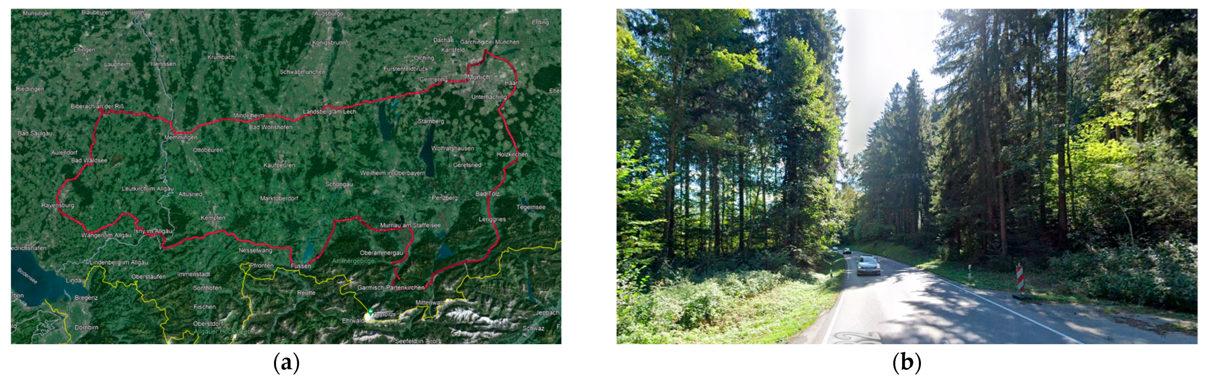
Additionally, kinematic PPP-RTK scenarios covering a total length of 600 km were recorded in Munich and included in the study, as shown in Figure 1. The route is illustrated in Figure 2. While the majority of the environment featured highway conditions, the scenario commenced in sub-urban surroundings. Additionally, the route passed through tree canopy and mountain areas, potentially degrading the solution quality. Figure 2 also provides an example of the environmental conditions encountered in the tree canopy areas.

A F9P U-blox receiver was employed, outfitted with an automative grade antenna. In these scenarios, reconvergences of the same duration were launched every 5 min, lasting 15 min each.

The forthcoming analysis compares results obtained with and without ionospheric corrections, with the objective of analyzing their respective impacts on the convergence time of PPP-RTKs. Additionally, the inclusion of the time taken to achieve specific errors by percentiles allows for an assessment of the impact of incorporating the global ionosphere model as corrections in PPP-RTK. It is worth noting that convergence was considered to have been achieved when the horizontal positioning error stabilized.

3. Results

3.1. Convergence Analysis in Static Scenarios: GPS Reference Stations

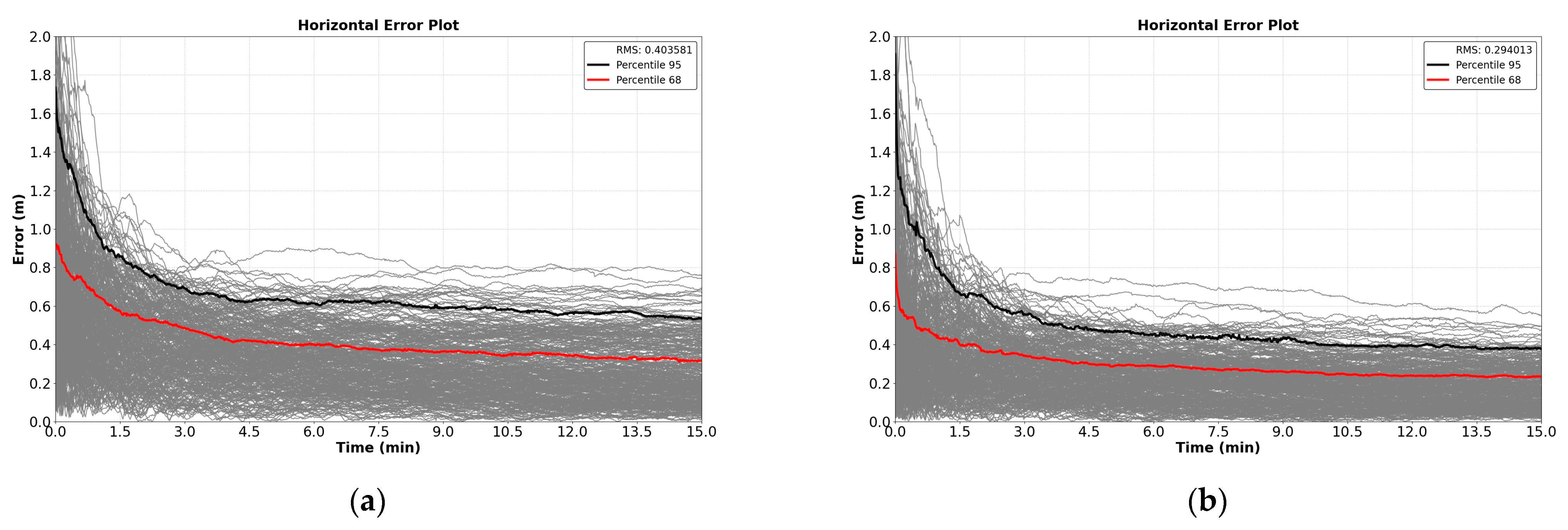
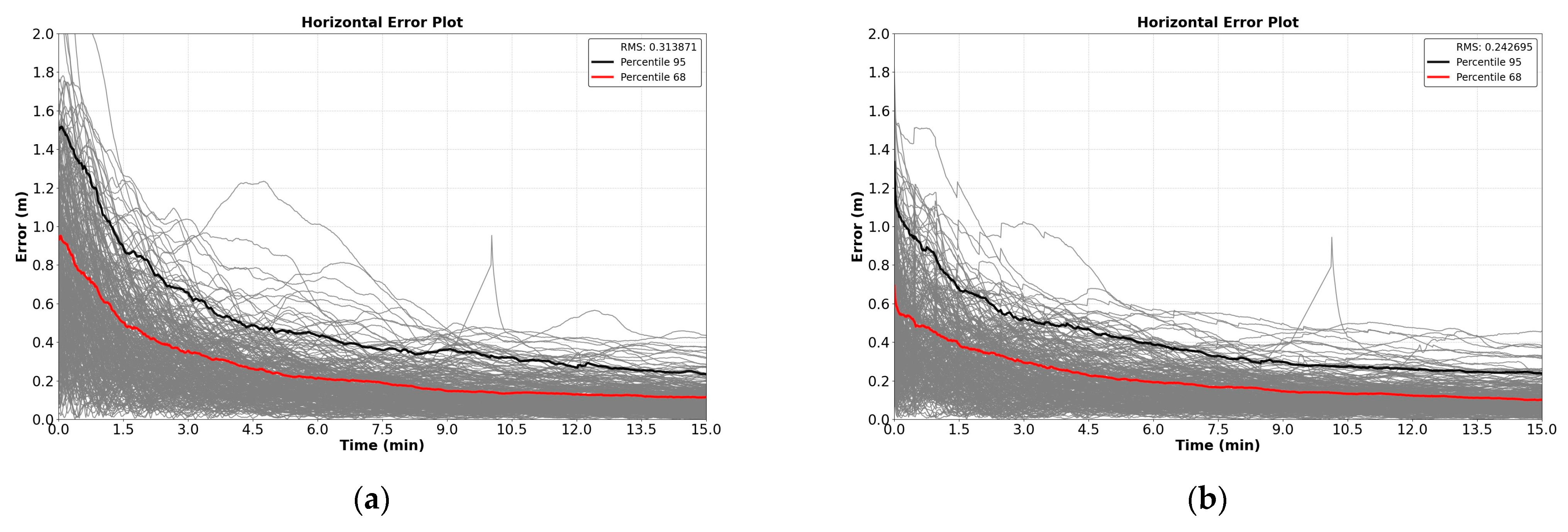
Figure 3 and Figure 4 represent the horizontal error values obtained during all convergence runs with and without ionosphere corrections for a one-week scenario at each GPS reference station. In Figure 3, the horizontal error values correspond to a station located in the eastern region of Europe. Meanwhile, Figure 4 presents the convergence results analyzed at a Korean station.

To summarize the results depicted in the preceding figures,

Table 1. Convergence time taken to achieve different levels of error without ionosphere corrections (No iono) and with ionosphere corrections (Iono) evaluated in GPS Reference Stations.

Station	Error (m)	68th Percentile		95th Percentile
		No Iono	Iono	No Iono	Iono
Eastern region of Europe	1	0 s	0 s	39 s	0s
	0.75	0 s	0 s	161 s	1 s
	0.5	120 s	1 s	343 s	203 s
	0.3	320 s	220 s	11 min	10 min
Korea	1	0 s	0 s	56 s	26 s
	0.75	25 s	2 s	132 s	71 s
	0.5	163 s	29 s	>15 min	221 s
	0.3	>15 min	270 s	>15 min	>15 min

collects the time to achieve 1, 0.75, 0.5, and 0.3 m by the 68th percentile and 95th percentile in convergences with and without ionospheric corrections for each station.

3.2. Convergence Analysis in Static Scenarios: U-Blox Receiver

The horizontal error values obtained when a F9P U-blox receiver was used as monitoring station are presented in Figure 5.

Table 2. Convergence time taken to achieve different levels of error without ionosphere corrections and with ionosphere corrections evaluated in U-Blox Receiver.

Station	Error (m)	68th Percentile		95th Percentile
		No Iono	Iono	No Iono	Iono
F9P U-blox receiver in Madrid	1	0 s	0 s	74 s	16 s
	0.75	36 s	0 s	134 s	74 s
	0.5	92 s	29 s	254 s	200 s
	0.3	237 s	177 s	11 min	8 min

presents information about percentile convergence time, following the same format as the previous cases.

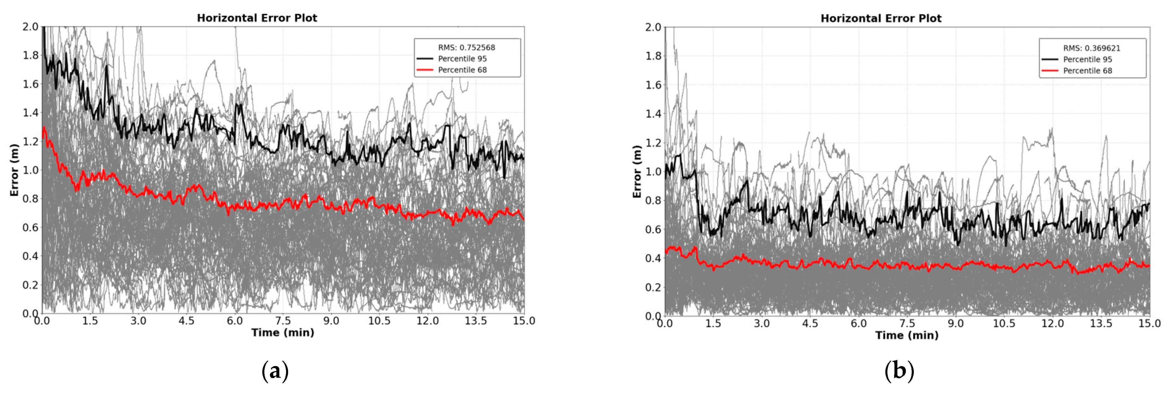
3.3. Convergence Analysis in Kinematic Scenarios

Figure 6 represents the convergence results obtained for a kinematic scenario recorded over 600 km. The convergence time taken to achieve 2, 1, 0.75, and 0.5 m by the 68th percentile and 95th percentile is summarized in

Table 3. Convergence time taken to achieve different levels of error without ionosphere corrections and with ionosphere corrections evaluated in Kinematic Scenarios.

Station	Error (m)	68th Percentile		95th Percentile
		No Iono	Iono	No Iono	Iono
F9P U-blox receiver in Munich	1	32 s	0 s	13 min	0 s
	0.75	332 s	0 s	>15 min	63 s
	0.5	>15 min	0 s	>15 min	9 min

.

4. Conclusions

This paper assessed the accuracy of global ionosphere model corrections on PPP-RTK across diverse scenarios. The results demonstrate a notable improvement in convergence time, especially evident when employing mass-market receivers. These results underscore the significance of incorporating global ionosphere model corrections to enhance the performance of PPP-RTK systems in real-time applications.

Furthermore, the model’s ability to achieve excellent performance with only 41 stations suggests that a large network of stations may not be necessary to reach this level of performance. Expanding the number of stations is expected to improve the model’s accuracy, leading to further enhancements in PPP convergence. However, this expansion would entail higher financial and infrastructural costs.

An additional advantage of this ionosphere model is its ability to approximate large data volumes with just a few coefficients. However, it is worth noting a drawback: the elimination of rapidly varying information over short periods.

As a potential future development, this model could be adapted as a regional model by expanding spherical harmonics in a specific geographic area. Focusing on a particular region would allow the model to better capture the dynamic behavior of the ionosphere, leading to more accurate ionospheric corrections. As a result, this could reduce the convergence time for precise point positioning (PPP).

References

- Kouba, J.; Héroux, P. Precise point positioning using IGS orbit and clock products. GPS Solut. 2001, 5, 12–28. [Google Scholar] [CrossRef]
- Sanz Subirana, J.; Juan Zornoza, J.M.; Hernández-Pajares, M. GNSS Data Processing, 3rd ed.; ESA Communications: Noordwijk, The Netherlands, 2013; pp. 109–121. [Google Scholar]
- GMV. Global GNSS Network Data Provision Service. Available online: https://magicgnss.gmv.com/magicGNSS_Reference_Network.pdf (accessed on 10 May 2024).
- Schaer, S. Mapping and Predicting the Earth’s Ionosphere Using the Global Positioning System. Ph.D. Dissertation, The University of Bern, Bern, Switzerland, 1999. [Google Scholar]
- Choi, B.-K.; Lee, W.; Cho, S.; Park, J.; Park, P.-H. Global GPS Ionospheric Modelling Using Spherical Harmonic Expansion Approach. J. Astron. Space Sci. 2010, 27, 359–366. [Google Scholar] [CrossRef]
- International GNSS Service. Enabling the Highest-Accuracy Usability of Openly Available GNSS Data & Products. Available online: https://igs.org/ (accessed on 10 May 2024).
- u-blox. ZED-F9P-04B Data Sheet. Available online: https://content.u-blox.com/sites/default/files/ZED-F9P-04B_DataSheet_UBX-21044850.pdf (accessed on 10 May 2024).