Abstract
This paper addresses the critical issue of unwanted interference in airborne GNSS receivers, crucial for navigational safety. Previous studies often simplified the problem, but this work offers a comprehensive approach, considering factors like Earth’s reflective properties, 3D calculations, and distinct radiation patterns. It introduces Spatial Interference Distribution Expression Heat-map and Operation Efficacy Plot graphs to visualize interference distribution along flight paths. The results highlight the significance of physical configuration and distance from interference sources on receiver performance. The algorithm developed can assess interference effects on GNSS receivers and aid in selecting optimal flight paths for minimal interference. This research enhances understanding and management of unintentional interference in airborne navigation systems.
Keywords:
GNSS; navigation; interference; spoofing; aircraft; antenna; radiation pattern; mathematical modeling; simulation; receiver 1. Introduction
Navigation has been integral to human existence, evolving from natural landmarks to celestial bodies for orientation, and the quest for precision led to the development of Global Navigation Satellite Systems (GNSSs) deployed by various nations that offer unparalleled precision, all-weather functionality, and global coverage, catering to diverse applications [1,2,3]. GNSS constellations, comprising satellites, have become indispensable for navigation across the globe, marking a significant milestone in human navigation history [4,5,6,7,8,9,10]. Global navigation systems face vulnerability to unintentional interference from various sources, ranging from homemade Ham Radios to powerful airport radars emitting harmonics. Despite International Telecommunication Union guidelines, unintentional interference persists, and it is an important source of threat to the reliability and availability of GNSS services. Previous studies lacked consideration for terrain and Source height, operating only in a 2D space. This paper presents a comprehensive mathematical model, addressing these limitations and incorporating best- and worst-case scenarios to assess the impact of unintentional interference on airborne GNSS receivers [11,12,13,14]. After reviewing relevant studies, this paper outlines the necessary assumptions in Section 3. Previous mathematical models are then refined to construct an appropriate algorithm in Section 4. Section 5 delineates the algorithm’s structure and interprets simulation outcomes. Operational concepts are discussed in the subsequent section utilizing Spatial Interference Distribution Expression Heat-map (SPIDEH) and operation efficacy plot (OEP) graphs. The paper concludes with profound insights into the problem and its outcomes.
2. Previous Works and Methods
Two relatively recent papers discuss the issue of GNSS assumptions parametrically, revealing a progressive understanding of the problem [13,14]. These studies have focused on the calculation of the received power, or PR, at a GNSS receiver’s antenna as a means to estimate its performance. To calculate the PR, the calculation of h(x), as the flight profile, and of g(θ), as the radiation pattern of a GNSS receiver’s antenna, is required. The altitude of the Source of unintentional interference, or hTX, should also be considered. The final PR has been reported as
where f is the frequency in hertz, c is the speed of light in the SI system, and Pj is the power of the transmitted signal [13]. This formulation considers the perspective effect of power distribution in a 2D environment. Four important assumptions are hidden in (1), and are summarized below: As the Path Gain Factor is missing in (1), the Earth has been assumed as ideally absorptive. As far as we know, the surface of the Earth shows both reflective and refractive properties [15,16], especially when the transmitter’s or the receiver’s altitude is small with respect to the altitude of the other. The reflection from the surface of the Earth causes the fading effect, called multipath fading [17]. The basic formulation of the Path Gain Factor can be found in almost any “antenna” and “propagation” textbook, such as [18]. To reduce the complexity of the calculations and to provide a better understanding of the underlying method of analysis, many works have modeled the airborne GNSS receiver’s flight profile in 2-dimensions [13,14]. While this assumption is true and general enough to perform mathematical modeling of the problem, it introduces some inherent limitations in using the model and its results, which will be discussed in Section 3. One of these limitations is the inability of the model to deal with real-world flight routes. To use this model, a real flight profile must be projected into two dimensions, which requires considerable computational effort. One of the direct consequences of the 2-dimensional flight profile assumption described above is the assumed 2-dimensional radiation pattern of the airborne GNSS antenna. The g(θ) value in (1) shows this, where θ is the Angle of Arrival (AoA) of the received signal. Even though the real antenna’s radiation characteristics are expressed with E-plane and H-plane radiation patterns, earlier studies use one of these patterns without explaining how to choose an appropriate pattern [13,14].
3. Justification of Assumptions
In real-world scenarios, the selection of a flying object’s flight profile in three dimensions is constrained by practical considerations and the capabilities of the flying system itself. Passenger aircraft typically maintain a flat trajectory for safety and mission requirements, whereas quadcopters exhibit greater agility, enabling sharp turns and rapid altitude changes. Previous studies have addressed this by focusing on sample flight profiles, such as the OH and DH profiles, which are particularly relevant for modeling the landing phase of quadcopters due to their vertical takeoff and landing capabilities [14]. To simplify the problem, it is assumed that the flying vehicle cannot rotate along its longitudinal axis. In other words, during a flight, the top of the flying vehicle is always “up”. This assumption, which can be traced in quadcopter-like flying vehicles, guarantees the orientation of the airborne GNSS antenna’s axis of radiation pattern with respect to the flight profile at any single point. Obviously, the propagation medium for this study is the Earth’s atmosphere, from a few meters to a few tens of kilometers above the surface. But, as far as we know, this medium is not homogenous. Various types of clouds, dust, changes in air pressure in different regions, and changes in air density at various altitudes are time-dependent parameters and are impossible to model generally. While their effect can be modeled in Link Budget calculations as attenuations [19], the first Best-Case Condition (BCC) assumption can be described as follows: the atmosphere is assumed to be clear and homogenous at any point and altitude.
With its more than 6000 km radius, the Earth appears to be almost flat and without curvature for a few tens of kilometers, especially when the selected flight profile is just higher than a few hundred meters for 98% of the flight time. The second BCC assumption is, therefore, to consider the Earth as flat, theoretically. This flatness means that the surface is not curved; there are no mountains, hills, valleys, etc.; and the Source is always in the line of sight of the airborne GNSS receiver. The surface of the Earth is also considered to be completely reflective. Such a surface causes severe multipath fading effects. The effect of this assumption is studied in this paper, and thus it is not categorized as a BCC or a Worst-Case Condition (WCC). To reduce the complexity of this study, some propagation-related effects are neglected [20].
In real-world applications, the Interference Signal can be defined as any radio frequency signal that changes the noise level of the receiver. A Source can also use various types of antennas, ranging from omni-directional to static or rotating directional antennas. This wide range of possible changes introduces complexity; to eliminate this unwanted and unnecessary complexity, an isotropic antenna pattern has been assumed as a BCC assumption. For any particular application, the actual radiation pattern of the Source can be replaced in the formulation. Modeling in three dimensions makes it possible to move a Source around and to locate it arbitrarily, as well as to select its altitude. These considerations are almost in compliance with what occurs in reality. A Source can be carried by cars (i.e., police cars), mounted on static helium-filled balloons (i.e., airborne communication nodes [21,22]), or placed at required altitudes using towers. The location and altitude of transmitters are, therefore, assumed to be selected arbitrarily.
Radiation Pattern of the Airborne GNSS Receiver’s Antenna
The radiation pattern of the GNSS receiver’s antenna can also be chosen arbitrarily. This uncertainty shows the necessity of solving the problem in its general form, which implies that the final algorithm should be able to accept any E-plane and H-plane radiation patterns with the desired resolution. The radiation patterns of antennas can be calculated using formulas found in textbooks [23] or using numerical calculations. However, both these calculations assume the antenna is in Free Space. In real-world applications, the antenna is always near “something”, i.e., the Earth, its mounting structure, a radome or cover, etc. These parasitic bodies change the calculated radiation patterns of antennas [18]. In the case evaluated here, the antenna is mounted inside an airframe, and so the airframe deforms the radiation patterns. The general approach of this paper to accept the E- and H-plane radiation patterns arbitrarily helps the model to be useful in real-world applications. However, due to the lack of information about real GNSS antennas, an algorithm to generate arbitrary radiation patterns has been developed and will be introduced in Section 4.2.
4. Mathematical Modeling
4.1. The 3-Dimensional Flight Profile
To produce a more comprehensive model of a 3-dimensional flight profile, a mathematical model developed in [13] was used as a basis. The final model can describe almost any arbitrary flight profile. The flight path altitude characteristics can be described as defined in [13], as
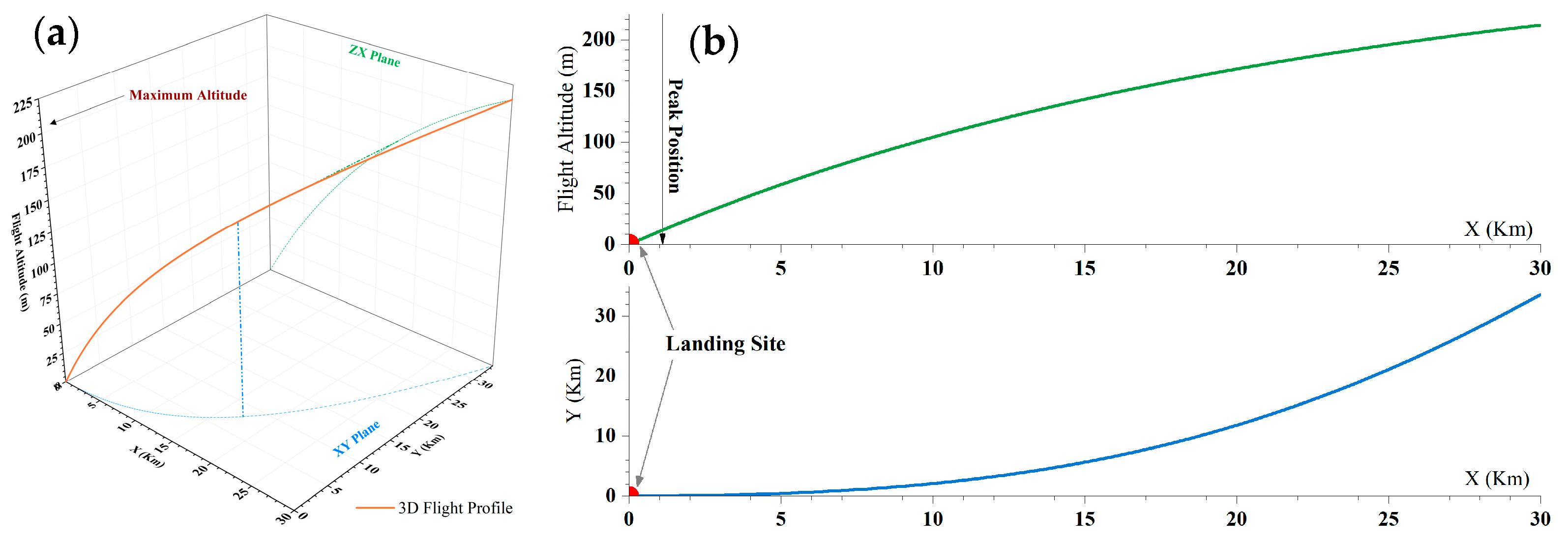
In which CPP, CCA, CMA, and CDF are defined as described in [13] and h(x) is an analytical function at any arbitrary point of x. Given that h(x) defines the altitude of the receiver, it can be associated with the z-axis of the 3D Cartesian coordination system. Let us assume y(x) = f(x), in which f represents any analytical function of x. Also, as the location of the landing site is considered to be located at (0, y(0), z(0)) = (0, 0, 0), the selected function, f, should satisfy f(0) = 0. In addition to the requirement of being analytical, f(x) should represent the real flight profiles of flying vehicles and comply with their aerodynamic capabilities and limitations. Figure 1 represents a sample flight. To simulate the landing flight phase, four essential variables of h(x) were adjusted as described in Table 1.
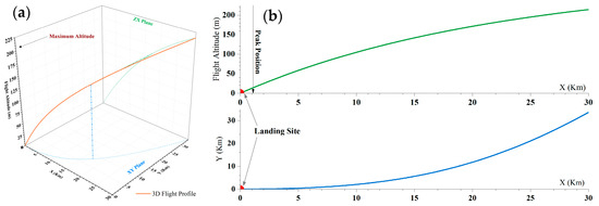
Figure 1.
(a). A sample flight profile with its projections in the XY and XZ planes. (b). The projection of the same sample flight profile in two perpendicular planes.

Table 1.
Parameters to set the Direct Landing (DL) scenario.
4.2. Radiation Patterns of a GNSS Receiver’s Antenna
Earlier works have only modeled the radiation pattern in the XZ plane. To generalize the study, the radiation patterns must be modeled in the XZ and XY planes as mathematical models of E- and H-plane radiation patterns, respectively. The selected models are based on what was used in [13], but with some modifications. These models are
In which C#,MLFZ, C#,BLS, C#,ST, C#,SP, and g#,max are defined as detailed in [13], but within their plane of projection (the # sign should be replaced with the XY or XZ terms). To assure the comparability of the results with those of earlier works, gXY and gXZ are modeled as described in [13], as listed in Table 2 and illustrated in Figure 2.
Table 2.
The suggested values for variables of (3) and (4).
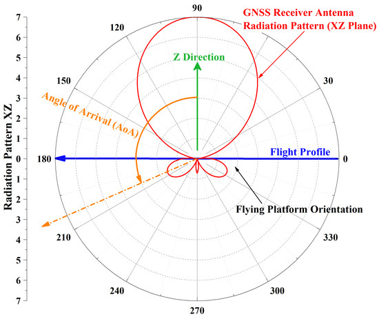
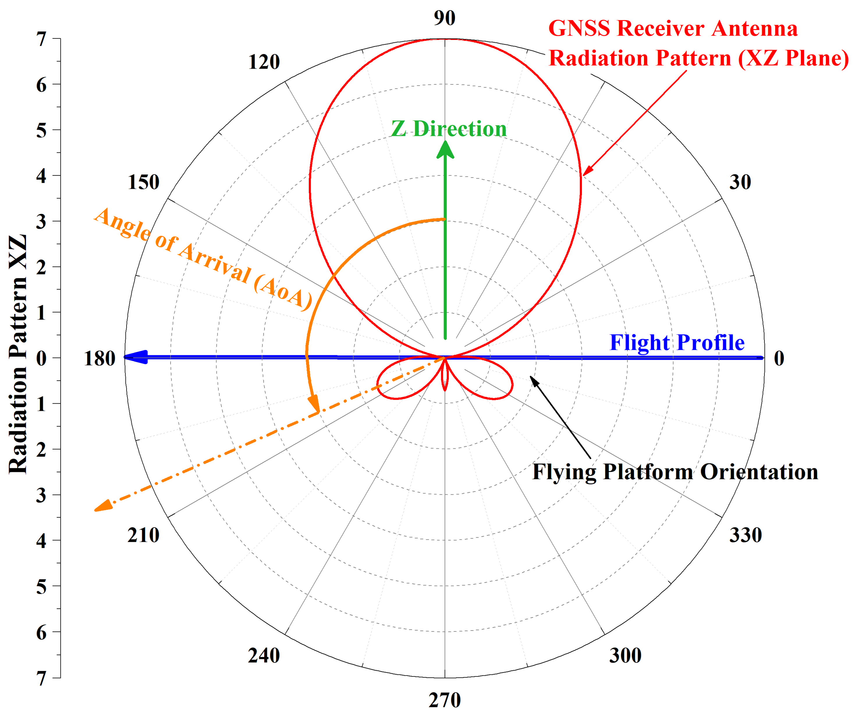
Figure 2.
The physical orientation of the GNSS receiver’s antenna and AoA.
4.3. Modeling the Angle of Arrival (AoA) and the Total Antenna Gain as a Function of the AoA
As assumed previously, the flying platform is assumed to be unable to rotate along its longitudinal axis. On the other hand, its longitudinal axis is tangential to the flight profile. Therefore, the mathematical derivation of the flight profile yields the values within which the E-plane and H-plane radiation patterns of the onboard GNSS antenna should rotate. As these radiation patterns correspond to the XZ and XY planes, it is sufficient to calculate the slope with respect to just two out of the three axes. Hence,
In addition, given that the Source can be located anywhere in the 3D space around the landing site, it can be logically justified to assume it to be located at any desired altitude (hTX ≥ 0). The line-of-sight (LoS) vector can then be translated from the landing site position to the Source position. Thus,
This vector should be rotated in accordance with (5) and (6), yielding
In (9), the [..] operator represents the floor function. The corresponding gains in the E- and H-planes are therefore gzy(AoAzy) and gzx(AoAzx), respectively. Finally, the final antenna gain in the direction of the received signal can be calculated as follows:
4.4. Modeling the Path Gain Factor and the Link Budget
The reflection of electromagnetic energy is highly dependent on the frequency, the incident angle, the material and physical composition of the surface, its roughness, etc. In this study, the Earth is assumed to be completely reflective, and its reflectance is assumed to be independent of frequency. As this assumption increases the effect of interference, it can be considered to be a Best-Case Condition for the unintentional Source of interference. Using this approach, the Path Gain Factor can be expressed as follows [18]:
where the |..| operator returns the absolute value of its argument and μ0 = 4π × 10−7 (F/m) and ε0 = 8.854 × 10⁻¹² (H/m) are the electrical permittivity and magnetic permeability, respectively, of the vacuum, and hTX is the altitude of the Source. The link budget can be calculated as follows:
In which PTX is the ERP of the Signal transmitter, GPath is the Path Gain Factor, GTX is the antenna gain of the Source in the direction of the AoA assuming GTX = 0, G is the receiver’s antenna gain in the direction of the AoA, and PRX is the received power, all in dBW.
5. Basic Results
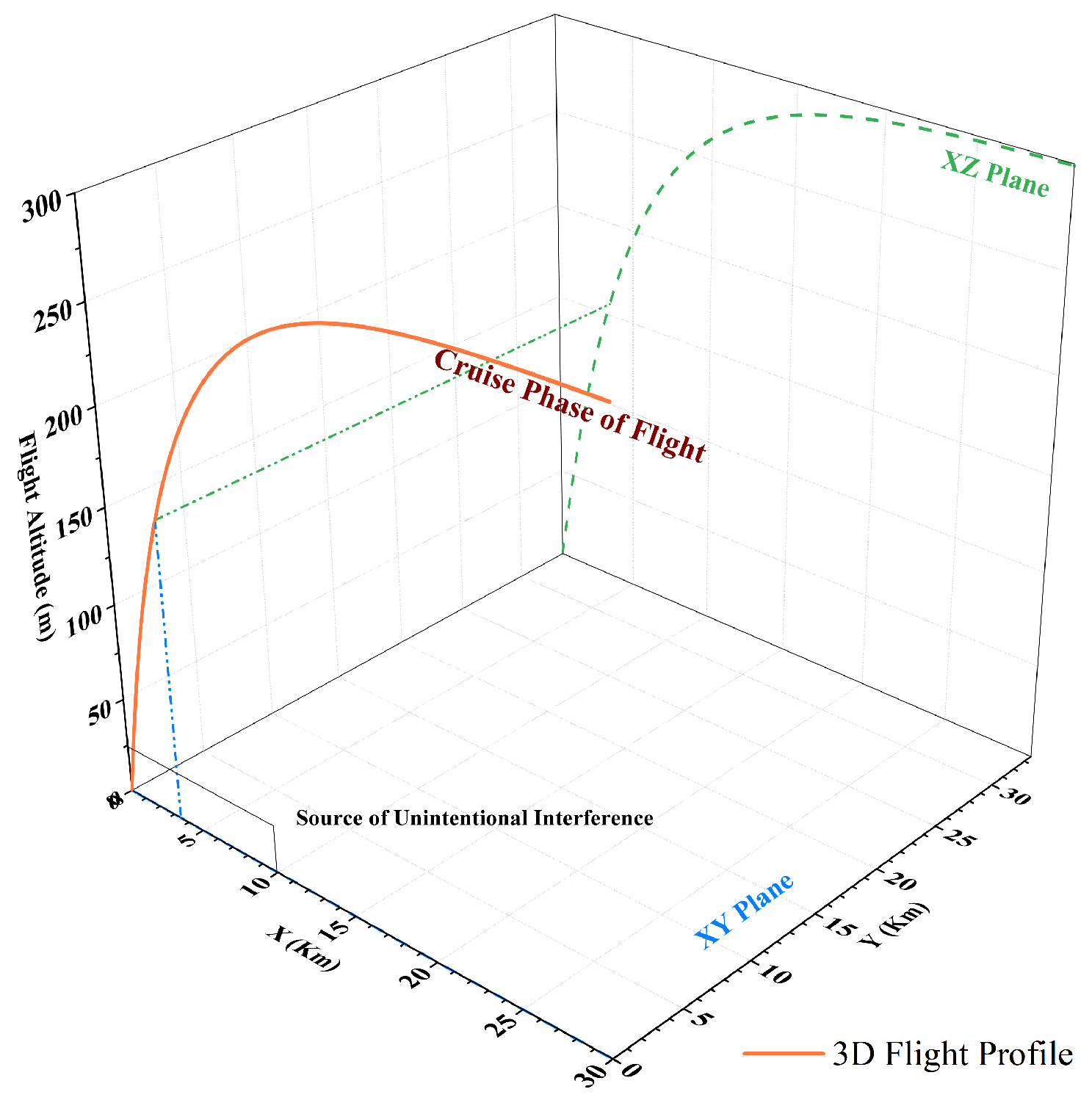
To study a simple case numerically, a DL scenario with y(x) = 0 was simulated by the suggested algorithm. The essential parameters of this scenario, the flight profile and the radiation pattern characteristics, are listed in Table 1 and Table 2, respectively. Figure 3 represents the flight profile of the airborne GNSS receiver. An unintentional Source of interference with an Effective Radiation Power (ERP) of 20 dBW and an isotropic antenna operates at (10, 0, 0.025). The installation/operational height of this transmitter can be selected arbitrarily, but the selected value is nominal for ground-based and mast-installed antennas. The graphical representation of the physical orientation of the radiation pattern of the GNSS antenna in the XZ-plane, the DoA and the AoA, are shown in Figure 3. If the XZ-plane is associated with the antenna’s E-plane, then the H-plane representation would be in the YZ-plane. In our case, as the dynamics of the flying platform requires the onboard GNSS receiver to be able to perform direction-independent navigation, the E- and H-plane radiation patterns were assumed to be identical, but they can be set arbitrarily or by using the measured values of real antennas.
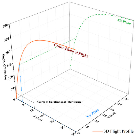
Figure 3.
A graphical representation of the selected landing scenario in 3D.
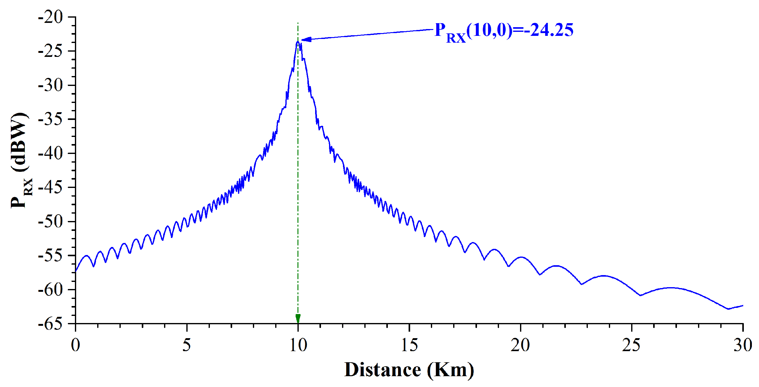
While Figure 2 simplifies the 3D representation of AoA in two dimensions, it should be noted that the DoA is a vector in a 3D space, and so it can be calculated directly from its XZ and XY (E- and H-plane) components. The calculated AoAs can be associated with their respective antenna gains in perpendicular planes. Also, to preserve the radiation patterns’ analytical aspect, any simulated radiation pattern must have identical E- and H-plane maximum values at their extremum points, i.e., at the patterns’ main lobe. In this case, these maximum values for the E- and H-planes are set at 7 dBi. The calculated PRX is shown in Figure 4. The PRX is higher when the flying platform is closer to the Source. The fluctuation in the calculated PRX is due to the multipath fading effect, represented in the sinusoidal terms of (11).
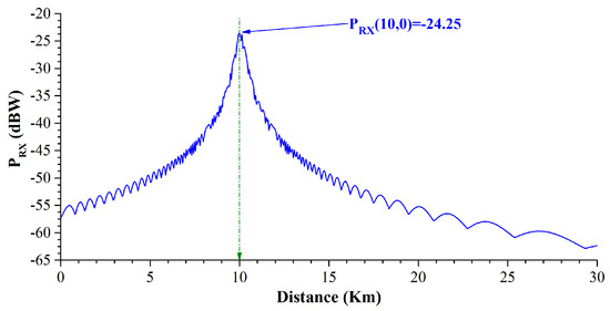
Figure 4.
The GNSS receivers received power from the Source for a landing scenario.
Angular Analysis and Optimized Flight Profile
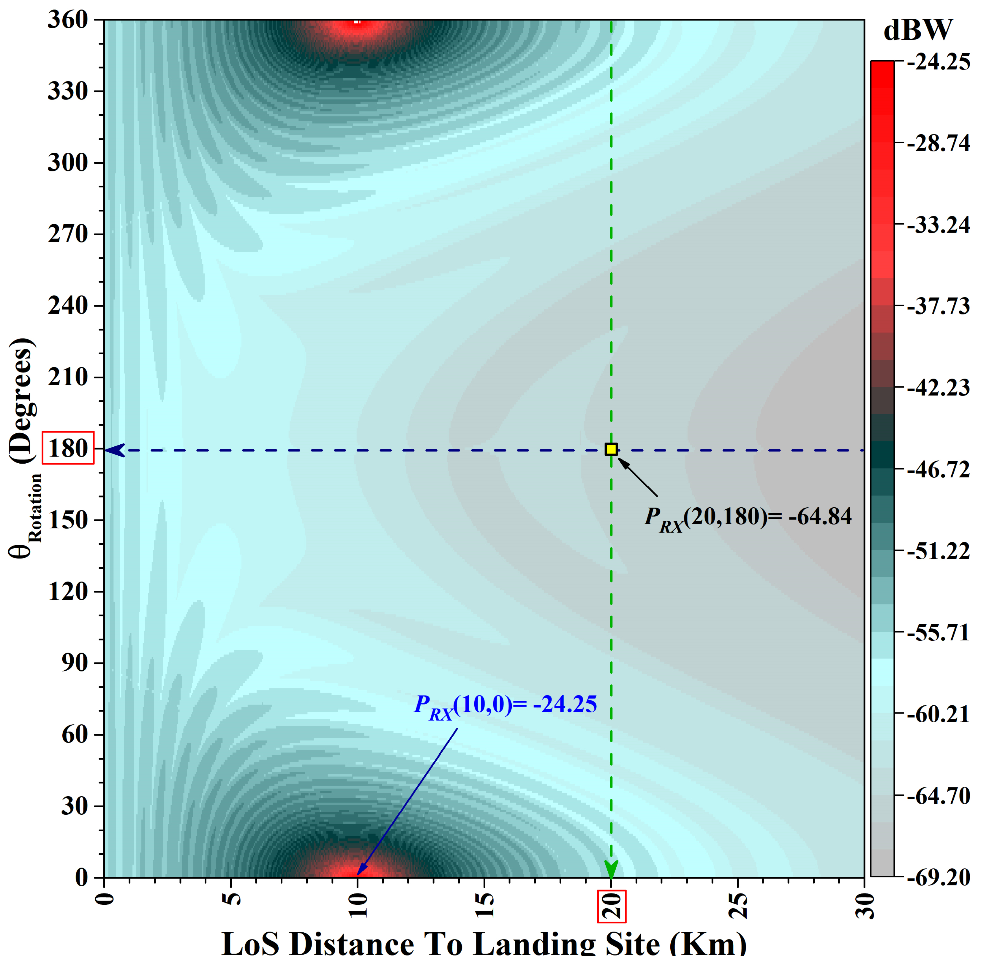
While all of these mathematical modeling and computational efforts were performed to calculate the PRX or the JSR along a flying platform’s flight path, the real-world applications are somewhat different. There is an essential question that the flying platform operator may ask: Is there an analytical approach to selecting a flight profile with “optimum” PRX that will retain the navigational capabilities of the onboard GNSS receiver? To answer this question, the flying vehicle operator must have some technical and tactical information about the Source. To reach justifiable results and to not diminish the generality of the study, it was assumed that this information is readily available, accessible, and valid. With the above-mentioned assumptions and considering the location and height of the Source as constant, the flight profile can be rotated along the z-axis at any desired resolution, called the Angular Resolution of the algorithm, and denoted as θR. On the other hand, the maximum distance for which the calculation will be performed is divided into sections, denoted as Δx. For this case, it was assumed that θR = 0.1° and Δx = 10 m. If θRotation = nθR, the PRX(mΔx, θRotation) for various values of n (covering [0, 2π)) and m (covering [0, 30 km]) were calculated and are illustrated in Figure 5. This plot shows useful and operation-oriented information about the PRX and its angular dependency and is known as a Spatial Interference Distribution Expression Heat-map (SPIDEH).
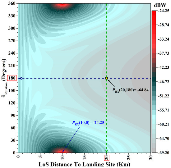
Figure 5.
The SPIDEH graph of a landing scenario. PRX(10, 0, 0.025), the maximum PRX(max) is at 10 km and θRotation = 0°.
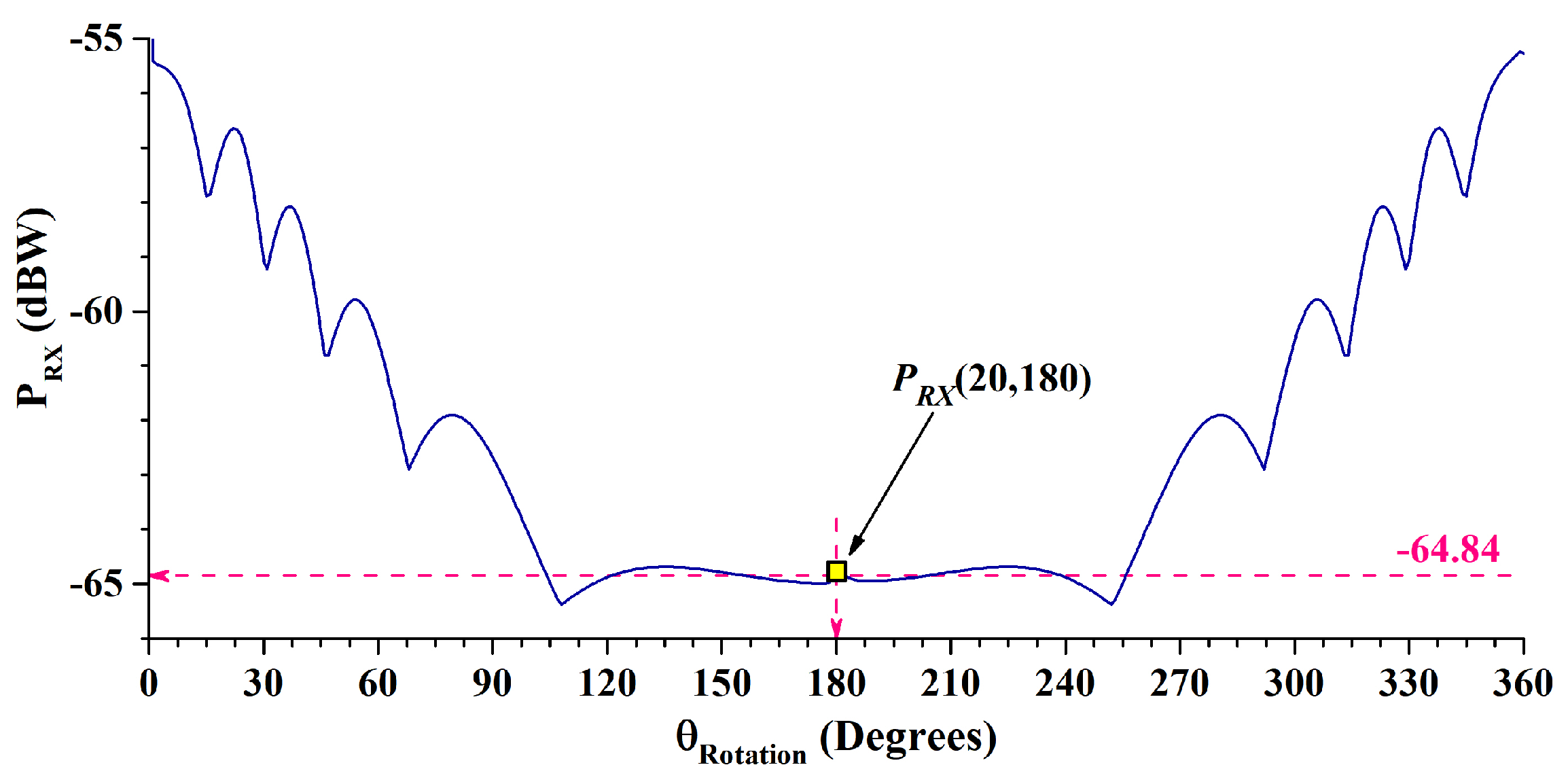
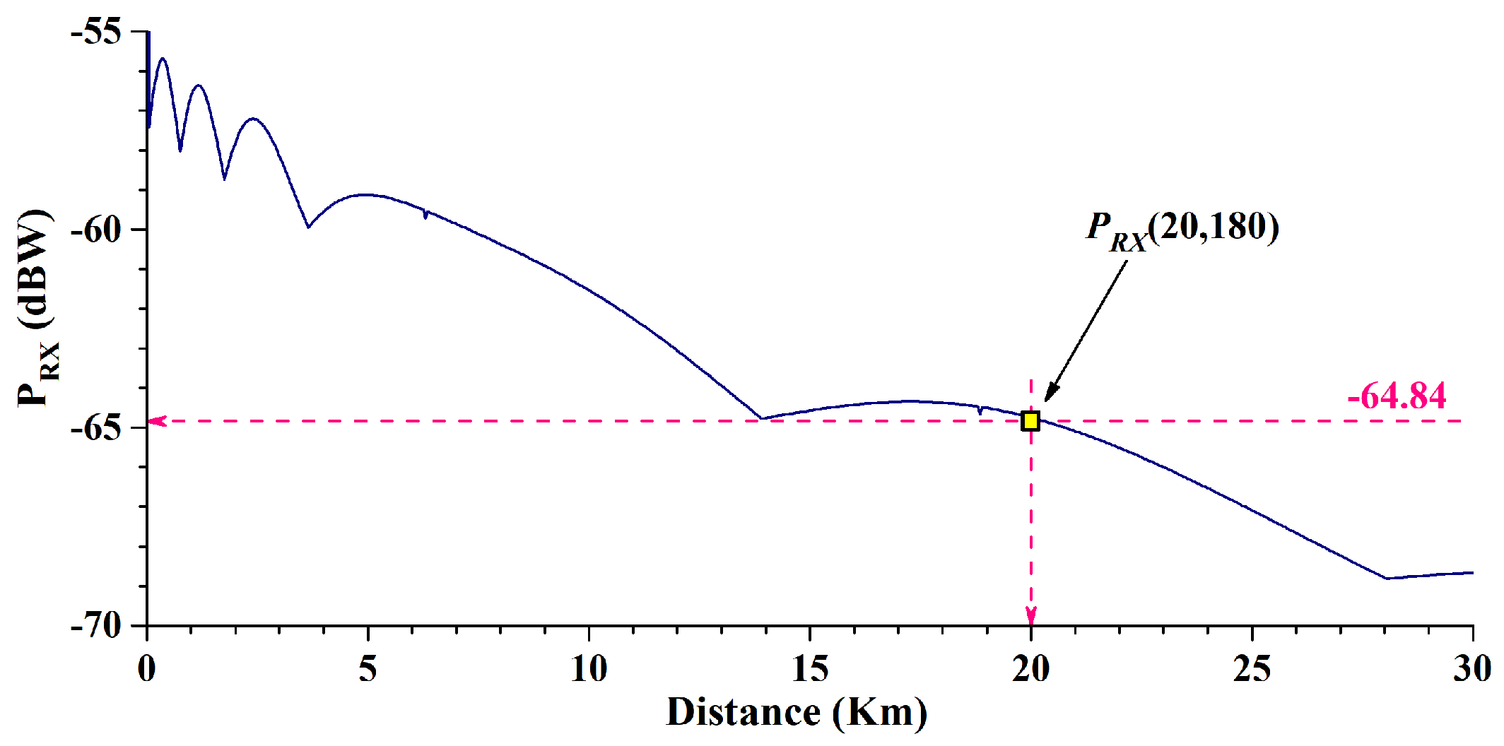
While a SPIDEH may appear to be complicated, the concept is simple: any horizontal line represents the PRX for the desired approach direction, and any vertical line relates to the various possible PRX values at the desired distances. For example, Figure 6 and Figure 7 represent the PRX (x = 20 km, θRotation = [0, 2π]) and PRX (x = [0, 30 km], θRotation = 180°), respectively. The horizontal axis of the SPIDEH graph, the x parameter, represents the line-of-sight distance of the flying platform from the landing site, or LoS-DtLS. The exact location can also be calculated. The SPIDEH graph shows two straight (dashed) lines. The intersection of these two straight lines at (20 km, 180°) are also represented in Figure 6 and Figure 7. The maximum value of PRX in Figure 5, PRX (10), can be represented in the SEPIDEH graph and is associated with PRX (10, 0°). This information implies that the curve of the receiver’s power in Figure 4 is a row of data at θRotation = 0° in a SEPIDEH graph. This type of representation contains enough information to answer the question about selecting an optimal flight pattern. The answer is the path or batch of paths with minimum values of PRX. As the starting point of this flight is somewhere 30 km away from the target, a simple search algorithm can find extremum values by scanning the [0, 2π) span of each mΔx of the SPIDEH graph. Figure 8 represents the results of calculating such an operation efficacy plot, or OEP. For a flying platform operator, it is essential to know the flight routes that have minimum JSR and to avoid those with a high probability of reducing the accuracy of the GNSS receiver. Figure 8 represents these two distinct regions. The minimum and maximum PRX for each x and various θRotation values are shown in blue and red, respectively. As the flying platform approaches the landing site within the blue region, the GNSS has repeated opportunities to update its navigational output. It is important to know that this plot shows the suggested regions, not the flight routes. The flying platform generally cannot follow the dotted path exactly due to limitations in its aerodynamic capabilities (i.e., no sharp turns to the left or right), fuel consumption, or other operational considerations. If the selected flight path is assumed to be set at θRotation = 150°, as shown with a green line in Figure 8, then the resultant PRX with the PRX of the original flight path (at θRotation = 150°) can be compared. This comparison is illustrated in Figure 9. In this case, the total received power for these two approach directions differ by an order of 4. Also, the local minimum values of PRX(θRotation = 150°), the blue radial patterns in Figure 8, are distanced enough to allow the GNSS receiver to update its navigational results.
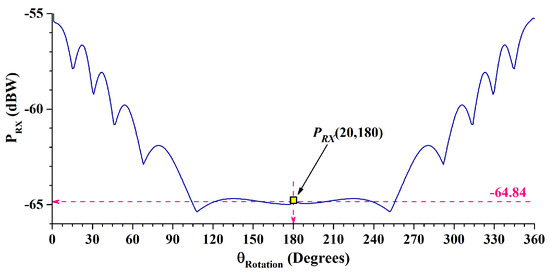
Figure 6.
Variation in PRX while a flying platform rotates around the landing site at LoS-DtLS = x = 20 km and at a fixed altitude of h(x). The location of these data are indicated in Figure 5 by the vertical dashed green line. By assuming a symmetric radiation pattern, this plot should also be symmetric.
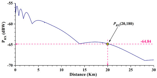
Figure 7.
Variation in PRX if a flying platform nears the landing site from θRotation = 180°.

Figure 8.
The operation efficacy plot of the landing scenario with a single source, located at (10, 0, 0.025).
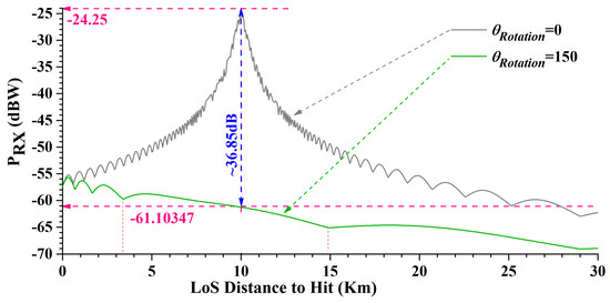
Figure 9.
A comparison of PRX for two angles of approach (for a selected landing scenario).
6. Discussion
6.1. Multipath Fading Effect
To evaluate the effect of Path Loss on the calculated PRX, consider a single point of measurement Pm = (xi, yi). In addition, the Source is assumed to be located at Pj = (xj, yj, zj). If Pm is rotated along the z-axis, then the relative distance between Pj and Pm varies. An example of such variation is illustrated in Figure 6. The figure is symmetric, which complies with the geometrical configuration. The reflective properties of Earth cause the fluctuations due to changes in the incident angles at various distances.
6.2. Effect of Distance Between Source and Landing Site
The maximum values of PRX are located around the jammer’s location regardless of whether the flight vehicle passes overhead or beneath the Source. So, if the Source is assumed to be located in the vicinity of the landing site, it can considerably deteriorate the navigational capabilities of the GNSS receiver, as indicated by the PRX graph in Figure 10. On the other hand, it should be noted that the GNSS is a secondary navigational tool in some real-world applications, while the INS is always the primary source of navigational information if it is being used.
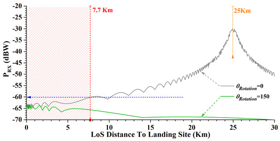
Figure 10.
When the Source is located at (25, 0, 0.025), it cannot provide a typical GNSS with strong enough PRX. For example, the maximum PRX that the GNSS receiver can compensate for is shown with a blue line at −60 dBW.
The accumulative navigational error of the INS system is part of why the GNSS receiver is needed, and also accounts for why a distant Source can also result in malfunctioning of the navigational pair of GNSS and INS. If a distant Source makes the GNSS navigational service unavailable, the INS will be unable to eliminate its internal error, and the blind-flying distance makes this error large enough to prevent the flying platform from reaching its landing site.
6.3. OEP vs. Source Location
As shown in all the represented OEP, the regions with the most and least power from the Source of unintentional interference (the areas containing red and blue dots, respectively) are always stretched along the line that connects the Source to the landing site, and they rotate if this line rotates. On the other hand, the relative distance between the Source and the landing site inversely affects the size of these regions and their separation. While the Pj = (0.75, 0, 0.025) causes an all-around mixture of these two regions, Pj = (5, 0, 0.025) makes these regions more focused and spatially separated.
6.4. GNSS Receiver’s Chance of Success
In OEP, the surface area of the blue regions is always bigger. The difference between surface areas can be interpreted such that if the approach direction is assumed to be selectable within (0, 2π), then it is possible to find suitable flight profiles to reduce the unwanted effect of unintentional interference. When considering the real-world characteristics of a typical GNSS receiver, the correctness of this interpretation is not always evident. It depends on the dynamic range of the GNSS receiver, and its ability to withstand the interfering signals and to compensate for a certain amount of PRX. As this information may not always be available, the only correct and sufficient interpretation is that the flying platform operator has more choices on how to reach the landing site with optimum reception of the signal from the single source of unintentional interference. Also, if the Source is assumed to be installed at higher altitudes, it might be able to insert more power into the GNSS receiver. At the same time, this configuration results in narrower blue and red regions.
6.5. Path Loss and Operational Considerations
As mentioned in various textbooks, while the reflective surface of Earth and the resultant multipath fading play a role in slightly degrading the Source to GNSS receiver link budget, the most considerable attenuation is due to the line-of-sight Path Loss and radial reduction in power density. Given that the GNSS receiver has a predefined dynamic range and can deliver accurate navigational information for up to a certain PRX, this degradation limits the maximum distance of the Source from the landing site to be considered effective. A sample case illustrating such a scenario is shown in Figure 10. The hashed red area indicates the distance of the flying platform from the landing site when the PRX value drops below the GNSS critical value. This is ~7.7 km, which can be passed in ~460 s at a speed of 60 km/h (a WCC assumption for a typical flying platform such as a quadcopter). During this time period, a 25 Hz GNSS receiver makes ~11,550 attempts to update its output. So, the GNSS receiver has an excellent chance to update its navigational output during its final phase of flight, and, logically, the effect of the interfering signal can be termed unsuccessful.
7. Conclusions
The pervasive use of location-finding services underscores their importance across various sectors, yet their susceptibility to RF interference remains a significant challenge. This paper addresses this concern by mathematically modeling the problem in a 3D space, focusing on GNSS receivers during the landing phase of flying vehicles. Incorporating factors like flight path, antenna radiation patterns, and multipath fading, the analysis employs SPIDEH and OEP graphs to elucidate PRX dependencies and operational insights. Simulations reveal the spatial arrangements of maximum and minimum PRX points, emphasizing the impact of distance between the Source and landing site. The results highlight the dynamic nature of PRX regions and unequal interference biases, suggesting avenues for future research on optimizing flight paths amidst interference.
Author Contributions
All authors have the same level of contribution. All authors have read and agreed to the published version of the manuscript.
Funding
This research received no external funding.
Institutional Review Board Statement
Not applicable.
Informed Consent Statement
Not applicable.
Data Availability Statement
Not applicable.
Conflicts of Interest
The authors declare no conflict of interest.
References
- Dachev, Y.; Panov, A. 21st Century Celestial Navigation Systems. In Proceedings of the 18th Annual General Assembly AGA, IAMU, Varna, Bulgaria, 11–14 October 2017. [Google Scholar]
- SR-71, An Online Aircraft Museum, The Blackbird Archive an In-depth Look at the A-12, YF-12, and SR-71, SR-71 Flight Manual, Section IV: Navigation and Sensor Equipment, Astro-inertial Navigation System—Tape 12. Available online: https://www.sr-71.org/blackbird/manual/4/ (accessed on 24 January 2025).
- Tsai, K.-C.; Tseng, W.-K.; Chen, C.-L.; Sun, Y.-J. Analytical Solution Method for Celestial Positioning. J. Mar. Sci. Eng. 2022, 10, 771. [Google Scholar] [CrossRef]
- Kapotis, E.; Symeonides, C. Learning from a Museum Exhibit: The Case of the 19th-Century Compensation “Gridiron” Pendulum. Phys. Teach. 2019, 57, 222. [Google Scholar] [CrossRef]
- Popkonstantinovic, B.; Miladinovic, L.; Stoimenov, M.; Petrovic, D.; Petrovic, N.; Ostojic, G.; Stankovski, S. Practical method for thermal compensation of long-period compound pendulum. Indian J. Pure Appl. Phys. 2011, 49, 10. [Google Scholar]
- Asche, G.P. The Omega System Of Global Navigation. In Proceedings of the 10th International Hydrographic Conference, Monaco, 10–22 April 1972. [Google Scholar]
- Pace, S.; Frost, G.; Lachow, I.; Frelinger, D.; Fossum, D.; Wassem, D.K.; Pinto, M. The Global Positioning System Assessing National Policies; Critical Technologies Institute, RAND: Santa Monica, CA, USA, 1995; ISBN 0-8330-2349-7. [Google Scholar]
- Dale, A.; Daly, P. The Soviet Union’s GLONASS Navigation Satellites. IEEE Aerosp. Electron. Syst. Mag. 1987, 2, 13–17. [Google Scholar] [CrossRef]
- Lu, J.; Guo, X.; Su, C. Global Capabilities of BeiDou Navigation Satellite System. Satell. Navig. 2020, 1, 27. [Google Scholar] [CrossRef]
- Hecker, P.; Bestmann, U.; Schwithal, A.; Stanisak, M. Galileo Satellite Navigation System: Space Applications on Earth; European Parliamentary Research Service, Scientific Foresight Unit: Brussels, Belgium, 2008; ISBN 978-92-846-3340-1.
- Schmidt, G.T. INS/GPS Technology Trends; NATO Documents, RTO-EN-SET-116; Massachusetts Institute of Technology: Cambridge, MA, USA, 2011. [Google Scholar]
- Azouz, A. GPS\INS Integration for Land Vehicle Navigation Application. In Proceedings of the Al-Azhar Engineering 10th International Conference, Cairo, Egypt, 24–26 December 2008. [Google Scholar]
- Esmaeilkhah, A.; Lavasani, N. Jamming Efficacy of Variable Altitude GPS Jammer Against Airborne GPS Receiver, Theoretical Study and Parametric Simulation. Adv. Electromagn. 2018, 7, 57–64. [Google Scholar] [CrossRef]
- Lavasani, N.; Esmaeilkhah, A. Mathematical Modeling of Efficacy of Ground-based Jamming Operation against Airborne GPS Receiver. In Proceedings of the 1st Conference on Modeling Mathematics & Statistics in Applied Studies, Chalus, Iran, 16 February 2017. [Google Scholar]
- Rüeger, J.M. Refractive Index Formulae for Radio Wave. In Proceedings of the FIG XXII International Congress, Washington, DC, USA, 22 April 2002. [Google Scholar]
- Stephens, G.; Gristey, J.J.; Schmidt, S. The Spectral Nature of Earth’s Reflected Radiation: Measurement and Science Applications. Front. Remote Sens. 2021, 2, 664291. [Google Scholar] [CrossRef]
- Mella, K. Theory, Simulation and Measurement of Wireless Multipath Fading Channels. Master’s Thesis, Norwegian University of Science and Technology, Trondheim, Norway, May 2007. [Google Scholar]
- Collin, R.E. Antennas and Radiowave Propagation; McGraw-Hill: New York, NY, USA, 1985. [Google Scholar]
- Hum, S.V. Radio and Microwave Wireless Systems, Atmospheric Effects; Wiley and Sons: Hoboken, NJ, USA, 2010. [Google Scholar]
- Dolukhanov, M. Propagation of Radio Waves; Editorial URSS: Moscow, Russia, 1995; ISBN 5884170823/9785884170827. [Google Scholar]
- Alsamhi, S.H.; Almalki, F.; Ma, O.; Angelides, M.C. Performance optimization of tethered balloon technology for public safety and emergency communications. Telecommun. Syst. 2022, 75, 235–244. [Google Scholar] [CrossRef]
- Vishal, M.; Taploo, A.; Thote, S.P. Airborne Internet Providing Tethered Balloon System, December. Int. J. Eng. Res. 2015, 4, 680–684. [Google Scholar] [CrossRef]
- Balanis, C.A. Antenna Theory: Analysis and Design, 4th ed.; John Wiley & Sons: Hoboken, NJ, USA, 2016; ISBN 978-1-118-64206-1. [Google Scholar]
Disclaimer/Publisher’s Note: The statements, opinions and data contained in all publications are solely those of the individual author(s) and contributor(s) and not of MDPI and/or the editor(s). MDPI and/or the editor(s) disclaim responsibility for any injury to people or property resulting from any ideas, methods, instructions or products referred to in the content. |
© 2025 by the authors. Licensee MDPI, Basel, Switzerland. This article is an open access article distributed under the terms and conditions of the Creative Commons Attribution (CC BY) license (https://creativecommons.org/licenses/by/4.0/).