Abstract
The increasing complexity of lunar exploration missions necessitates stricter navigation requirements, especially when human life is involved. Extensive research is currently being conducted on various positioning systems suitable for the lunar environment. These include both the exploitation of terrestrial GNSS (Global Navigation Satellite System) signals, and the deployment of a lunar-dedicated satellite system known as the Lunar Communication and Navigation Service (LCNS). In order to meet the demanding navigation requirements, the usage of one or more lunar beacons to enhance Positioning, Navigation, and Timing (PNT) performance for different assets is under investigation to complement the LCNS system. This research aims to demonstrate the improvement of PNT accuracy by exploiting Differential LCNS (DLCNS) positioning techniques. To this end, both Single Point Positioning (SPP) and DLCNS techniques along with estimation algorithms such as Weighted Least Squares (WLS) and Extended Kalman Filter (EKF) were developed in a simulated lunar environment to assess their performances.
1. Introduction
The exploration of the Moon has been a topic of great interest in recent times, thanks to the discovery of valuable resources such as ice-water on the lunar surface. This has reignited the ambition to establish a human presence on the Moon within the next decade. However, the complexities associated with lunar exploration missions necessitate the development of more robust navigation systems, particularly when human life is involved. In recent years, numerous studies have been published assessing the potential use of GNSS signals for lunar navigation [1]. Furthermore, in 2019 the Magnetospheric Multiscale (MMS) mission received GPS signals at 187,166 km, i.e., almost half of the Earth–Moon distance [2]. However, this approach presents various challenges, including poor satellite geometry and small signal power available on the lunar surface coming from the side lobes of GNSS satellites. For this, many efforts have focused on the deployment of a dedicated lunar satellite system. In this context, ESA proposed the LCNS as part of the Moonlight program. Several studies have been conducted to evaluate the navigation performance achievable on the Moon surface and in orbit. For example, [3] assesses PVT accuracy during a typical moon landing using a dedicated lunar satellite constellation exploiting undifferenced measurements. Furthermore, [4] investigates the potential of differential LCNS techniques, employing both code and phase measurements with the integration of a DEM (Digital Elevation Model).
In the context of this second lunar race, this study aims to demonstrate how the deployment of a lunar beacon can contribute to the enhancement of navigation performance obtainable with a LCNS constellation, enabling the use of different DLCNS techniques and without any additional sensors.
2. Simulation Scenario and Methods
2.1. Simulation Scenario
The satellite constellation employed in the analysis comprises four satellites deployed in ELFO (Elliptical Lunar Frozen Orbit) orbits. These orbits are designed to stay practically fixed, thereby minimizing the fuel consumption required for station keeping. Furthermore, they are able to provide eight hours of continuous coverage, minimizing the PDOP (Position Dilution of Precision) of the lunar South Pole. The orbital parameters of the satellites are presented in Table 1.

Table 1.
Orbital parameters of the LCNS constellation.
Simulations were carried out in the following time window:
- Start time: 4 September 2020 18:00:00
- Stop time: 5 September 2020 02:00:00
- Step time: 1 s
The lunar beacon reference position is set in the proximity of the lunar South Pole with latitude, longitude, and altitude values set to: −89 degrees, 0 degrees, and 100 m, respectively. The lunar user is situated at an approximate distance of 2 km from the beacon and remains static. This configuration is designed in such a way that the user is able to receive the beacon signal, thereby enabling the exploitation of differential corrections and double-differenced measurements, given that the LOS (Line of Sight) range for the lunar beacon signal is approximately 10 km. A dynamic user has also been analyzed; however, without the implementation of the receiver chain, the tracking process is not accounted for, resulting in both users achieving the same PVT performance. For this reason, only static user results will be presented.
2.2. Measurement Modeling
To simulate pseudo-range measurements, an error model was introduced, to represent the various type of errors that affect these measurements. In particular, the following sources were of error taken into account:
- Clock errors: It is assumed that the clock model for the satellites, lunar beacon, and users are linear and composed of two terms: clock bias and clock drift;
- Receiver noise: This noise consists of two components: DLL (Delay-Locked Loop) error and jitter;
- Position error: The reference position of the beacon is assumed to be determined using Lunar Laser Ranging (LLR) techniques, which typically achieve an accuracy of approximately 0.2 m. However, for this analysis, a more conservative value is used (see Table 2). The position error of the lunar beacon is considered when calculating differential corrections and the precision of these corrections is highly influenced by this error;
Table 2. Error model. (All values are 1-sigma.)
- Ephemeris error: This error arises from inaccuracies in the satellite’s OD (Orbit Determination) process. Although it does not directly influence the pseudo-range simulations, it is introduced into the propagated satellite orbits to generate simulated orbits, thereby reproducing the effect of biased OD techniques.
- Internal studies were conducted to initialize the values of the error budget for the user, lunar beacon, and satellite, which are presented in Table 2.
The impact of the time-varying components of clock error has been considered negligible compared to the deterministic component and measurement noise. However, the evaluation of stochastic clock error components will be incorporated in future developments of this work. Therefore, the simulated pseudo-range measurement is expressed as
Figure 1 illustrates the PDOP for the static user. Given the close proximity between the lunar beacon and the user, the PDOP can be considered representative for both assets.
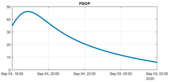
Figure 1.
PDOP computed at the static user location during the simulation time span.
2.3. Positioning Algorithms, Differential Corrections and Double Differences
In this work, two different estimation algorithms, namely WLS and the EKF, are used. Additionally, PNT solution is computed exploiting undifferenced, double-differenced, and corrected pseudo-ranges.
2.3.1. Weighted Least Squares
The WLS algorithm fits the available observations with a nonlinear model composed of four unknowns (three for position and one for the receiver clock offset) to estimate the user’s position. As a batch estimation method, WLS computes the solution independently at each epoch, without statistical correlation between past and future observations. The navigation equations are linearized to solve the positioning problem, and no dynamic model is applied. Further details on the WLS algorithm can be found in reference [5]. For pseudo-range measurements, the weight matrix is based on satellite elevation and is diagonal, assuming that all the measurements are independent. The diagonal components of the weight matrix are expressed as follows:
where represents the elevation of the i-th satellite.
In the case of double-differenced measurements, the weight matrix should not be diagonal due to the correlation arising from the combination of pseudo-range observations. In this work, however, it is simplified to the identity matrix (hence, reducing the WLS to a typical Least Squares algorithm). This approach has been adopted also in [6] and [7]. Such a correlation study is out of the scope of this work and will be integrated in the next developments.
2.3.2. Extended Kalman Filter
The EKF is one of the most widely used estimation algorithms for nonlinear systems, especially in navigation and positioning applications. By updating state and covariance estimates, the EKF is capable of providing accurate estimates in the presence of a nonlinear model and uncertainties in the system. The EKF is a predictive-corrective algorithm that operates in two steps:
- Prediction Step: The EKF propagates the state vector and its uncertainty, i.e., the state covariance matrix, based on the system’s model through the state transition matrix F;
- Update Step: When new measurements become available, the EKF updates the predicted state and its uncertainty through the Kalman gain, which optimally combines the predicted state with the measurements, also taking into account their noise.
The measurement covariance matrix R reflects the uncertainty in the measurements, while the process noise covariance matrix Q addresses uncertainties in the dynamics of the system being modeled. For this study, a constant acceleration model, like the one in [8], was selected due to its suitability for both static and dynamic scenarios. Additionally, a linear clock model with constant drift [8] was assumed, as the one presented in Equation (1). The EKF is applied to both undifferenced and double-differenced pseudo-ranges, necessitating different formulations of R and Q for each case. The measurements covariance matrix, under the assumption of no correlation between measurements in both cases, is expressed as follows:
It is assumed that there is no elevation dependency to reduce computational cost. Moreover, the standard deviation of double-differenced pseudo-ranges is twice the one of undifferenced pseudo-ranges. This is caused by the combination of observations as reported in [9]:
On the other hand, the process noise covariance matrix has been derived after the tuning of the filter. The selected form for it is as follows:
As will be presented in Section 2.3.4, the clock model is not accounted for when exploiting double-differenced measurements, since no receiver clock model has to be estimated. This matrix is practically composed of two submatrices, one with the position, velocity, and acceleration terms (Qx), and one for the clock model uncertainties (Qt), as illustrated below:
Following the tuning phase of the filter, the model uncertainty for acceleration was selected to be , while the values for the clock model parameters, namely the clock bias and drift, were set at and , respectively, as indicated in the specifications of the AXI-OM6060 clock by Axtal [10]. Finally, the filter is initialized with the initial conditions presented below in Table 3, which has also been retrieved after the tuning process of the filter.
Table 3.
Initial guess of the EKF.
2.3.3. Differential Corrections
Differential techniques aim to improve the accuracy of stand-alone LCNS positioning, one way of achieving this is to evaluate the errors in the reference station’s position solution (i.e., the lunar beacon) and transmit the corresponding pseudo-range corrections to the user’s receiver. The lunar beacon computes its position using signals from the LCNS and compares it with its reference position. The position error can be determined as a simple vector difference:
This position difference is then mapped into pseudo-range corrections using the design matrix H, which contains the cosine direction vectors between the satellites and the beacon:
The receiver receives and applies these corrections to the pseudo-range measurement of the same satellites, resulting in an increase in measurement noise by a factor of [9]:
2.3.4. Double Differences
An alternative DLCNS approach is the generation of double-differenced pseudo-ranges, also called DD (double differences). This method starts with the pseudo-range equations for two receivers considering the same satellite, as illustrated in Equation (2):
where Q represents the receiver noise, comprising jitter and DLL terms.
A SD (single difference) is derived by subtracting the two equations:
In the SDs formulation, the satellite clock bias cancels out; moreover, it is possible to differentiate two SD equations, thereby generating double differences:
With the formation of DD, the receiver clock bias cancels out too, so the only term remaining is the receiver noise Q that will be dropped for the sake of simplicity in further analysis. The three DD equations (from four satellites) give the following system:
The solution to this problem, as well as for the SPP, is obtained using the WLS. Moreover, it is possible to use these measurements in the framework of the EKF too. A more accurate description of DD formulation can be found in [5].
3. Results
This section presents the results obtained from the simulations. A Monte-Carlo-like approach was employed, performing 1000 simulations of the measurements. In each plot, the 95th percentile of every epoch is shown. Due to computational reasons, the EKF is re-initialized every two hours.
3.1. Single-Point Positioning (SPP)
Undifferenced pseudo-range measurements were processed using both the WLS and EKF. The results are provided below in Figure 2 and Figure 3:
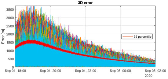
Figure 2.
SPP solution with WLS.
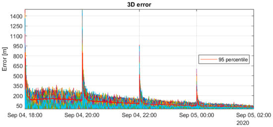
Figure 3.
SPP solution with EKF.
The accuracy of PVT solution has a strong dependence on the PDOP trend, with a slight difference between the two methods. While WLS results are highly sensitive to PDOP variations, EKF also depends on PDOP but benefits from the presence of the dynamic model, which can mitigate the effect of bad satellite geometry conditions. Moreover, from the values reported below in Table 4, it is evident that the implementation of the EKF brings out a strong enhancement of the position accuracy, since it filters all the AWGN uncorrelated error terms injected into the measurements. Indeed, this enhancement in the 3D accuracy is in the order of 89%.
Table 4.
95th percentile of the SPP solutions. All the values refer to the 95th percentile computed over the whole simulation.
3.2. DLCNS Corrections
The WLS algorithm is used again with corrected pseudo-ranges to improve the positioning accuracy in comparison to the SPP WLS solution. The results obtained with these corrected pseudo-ranges are illustrated in Figure 4:
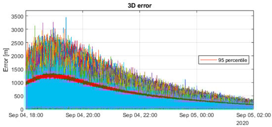
Figure 4.
Position solution with DLCNS corrections using WLS.
The principal advantage of pseudo-range corrections is that errors common to both receivers, such as satellite clock biases, cancel out, thereby enhancing overall positioning accuracy in comparison to the standard SPP WLS solution shown in Section 3.1. Furthermore, the solution trend still reflects the PDOP one.
A comparison of the results presented in Table 5 with those of Table 4 reveals that the use of DLCNS corrections has resulted in an enhancement in accuracy of approximately 18%, with the 3D error decreasing from 1511.40 m to 1238.28 m.
Table 5.
The 95th percentile of the position solution with DLCNS corrections. All the values refer to the 95th percentile computed over the whole simulation.
3.3. DLCNS Double Differences
The final positioning technique under consideration involves the use of double-differenced pseudo-ranges, which cancel out both satellite and receiver clock errors, thus, eliminating the receiver clock as an unknown variable. Below in Figure 5 and Figure 6, the results obtained with both WLS and EKF are presented.
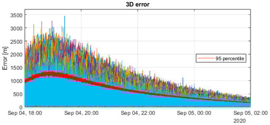
Figure 5.
DLCNS solution with WLS double differences.
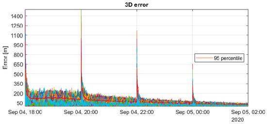
Figure 6.
DLCNS solution with EKF double differences.
A review of the values of Table 6 shows that, using WLS, there is a minimal difference between the DLCNS corrections solution and the one obtained with double-differenced pseudo-ranges. Furthermore, EKF applied to this combination of observables is the technique that provides the most accurate solution. The difference in the 3D accuracy yielded by the two algorithms in this case is around 89%.
Table 6.
The 95th percentile of the DLCNS solution with double differences. All the values refer to the 95th percentile computed over the whole simulation.
4. Discussions
In this study, various analyses were presented to examine two distinct positioning techniques, SPP and DLCNS, employing different estimation algorithms, namely WLS and EKF. The observations were simulated with the implementation of an error model, mostly composed of Gaussian terms. This enhances the performance of the EKF, which filters out uncorrelated Gaussian noise, resulting in an approximate 89% improvement in 3D positioning accuracy compared to the reference solution obtained with WLS in both SPP and DLCNS modes. The principal objective of this study was to assess the efficacy of employing DLCNS techniques to improve positioning accuracy. The first approach involved computing differential corrections to generate corrected pseudo-ranges, which were then processed using WLS. This method resulted in a 32% improvement in 3D accuracy, largely due to the cancelation of satellite clock errors. Then, the combination of pseudo-range measurements yielded double-differenced observables, which eliminate both satellite and receiver clock errors. The results obtained with WLS were comparable to those obtained with differential corrections, suggesting that the increased noise resulting from the combination of measurements may contrast the benefits of DLCNS. However, with EKF, the improvement with respect to the use of undifferenced observations is approximately 18%, achieving an overall accuracy of around 130 m in the 3D positioning. Note that the solution is influenced by satellite geometry and that, in the last two hours of the simulation, the 3D accuracy as it can be seen in Figure 6 reaches values around 50 m.
5. Conclusions
This study explores various positioning techniques within a lunar scenario, comparing SPP and DLCNS and exploiting different estimation algorithms like WLS and EKF, applied to simulated measurements. Results indicate that DLCNS combined with EKF significantly improves position accuracy, showing a nearly 90% reduction in error in 3D positioning compared to SPP with WLS. Moreover, the choice of positioning techniques and estimation algorithms significantly affects the accuracy of the position solution. The study emphasizes the importance of DLCNS in the lunar environment due to its ability to combine measurements and mitigate common error terms, leading to more precise solutions and going towards stringent navigation requirements for various missions.
Author Contributions
Conceptualization, M.F. and J.C.; methodology, M.F.; software, A.M.; validation, L.M.; writing—original draft preparation, A.M.; writing—review and editing, J.C. and M.F. All authors have read and agreed to the published version of the manuscript.
Funding
This research received no external funding.
Institutional Review Board Statement
Not applicable.
Informed Consent Statement
Not applicable.
Data Availability Statement
The data presented in this study are available upon request from the authors.
Conflicts of Interest
All authors were employed by the company Thales Alenia Space Italia and declare that the research was conducted in the absence of any commercial or financial relation-ships that could be construed as a potential conflict of interest”.
References
- Capuano, V. GNSS-Based Navigation for Lunar Missions. Ph.D. Thesis, Ecole Polytechnique Federale de Lausanne, Lausanne, Switzerland, 19 August 2016. [Google Scholar]
- Delépaut, A.; Giordano, P.; Ventura-Traveset, J.; Blonski, D.; Schönfeldt, M.; Schoonejans, P.; Aziz, S.; Walker, W. Use of GNSS for lunar missions and plans for lunar in-orbit development. Adv. Space Res. 2020, 66, 2739–2756. [Google Scholar]
- Grenier, A.; Giordano, P.; Bucci, L.; Cropp, A.; Zoccarato, P.; Swinden, R.; Ventura-Traveset, J. Positioning and Velocity Performance Levels for a Lunar Lander using a Dedicated Lunar Communication and Navigation System. Navig. J. Inst. Navig. 2022, 69, 2. [Google Scholar] [CrossRef]
- Psychas, D.; Audet, Y.; Melman, T.; Swinden, R.; Giordano, P.; Ventura-Traveset, J. On the Performance of LCNS-Based Differential Positioning on the Moon. In Proceedings of the ION 2024 Pacific PNT Meeting, Honolulu, HI, USA, 15–18 April 2024. [Google Scholar]
- Kaplan, E.; Hegarty, C. Understanding GPS/GNSS Principles and Applications, 3rd ed.; Artech House: Boston, MA, USA, 2017. [Google Scholar]
- Schielin, E.; Dautermann, T. GNSS based relative navigation for intentional approximation of aircraft. Aviation 2015, 19, 40–48. [Google Scholar]
- Dautermann, T.; Korn, B.; Flaig, K. GNSS Double Differences Used as Beacon Landing System for Aircraft Instrument Approach. Int. J. Aeronaut. Space Sci. 2021, 22, 1455–1463. [Google Scholar]
- Sarunic, W. Development of GPS Receiver Kalman Filter Algorithms for Stationary, Low-Dynamics, and High-Dynamics Applications. Defence Science and Technology Group Edinburgh Australia. Available online: https://www.dst.defence.gov.au/sites/default/files/publications/documents/DST-Group-TR-3260.pdf (accessed on 10 January 2024).
- Sansò, F.; Betti, B.; Albertella, A. Positioning. Posizionamento Classico e Satellitare, 3rd ed.; Città Studi Edizioni: Turin, Italy, 2019. [Google Scholar]
- Melman, F.T.; Zoccarato, P.; Orgel, C.; Swinden, R.; Giordano, P.; Ventura-Traveset, J. LCNS Positioning of a Lunar Surface Rover Using a DEM-Based Altitude Constraint. Remote Sens. 2022, 14, 3942. [Google Scholar] [CrossRef]
Disclaimer/Publisher’s Note: The statements, opinions and data contained in all publications are solely those of the individual author(s) and contributor(s) and not of MDPI and/or the editor(s). MDPI and/or the editor(s) disclaim responsibility for any injury to people or property resulting from any ideas, methods, instructions or products referred to in the content. |
© 2025 by the authors. Licensee MDPI, Basel, Switzerland. This article is an open access article distributed under the terms and conditions of the Creative Commons Attribution (CC BY) license (https://creativecommons.org/licenses/by/4.0/).