Abstract
The increasing global demand for air travel over the past three decades has led to heightened congestion, environmental concerns, and operational inefficiencies. This study explores the potential of commercial aircraft formation flight, inspired by the energy-saving flight patterns of migratory birds, to enhance fuel efficiency on the busy Melbourne to Sydney city-pair route. The methodology is divided into macroscopic and microscopic levels, addressing both strategic planning and detailed flight optimisation. The macroscopic level focuses on route optimisation, formation flight planning, air traffic management integration, and environmental impact. The microscopic level involves adjustments to individual aircraft flight profiles to ensure minimum separation, flight safety, and efficiency. Using a gradient-based optimisation algorithm applied to a constrained nonlinear multivariable function, this study aims to minimise fuel consumption and travel time while maintaining the required separation distances. The mathematical formulation and algorithm pseudocode provides a clear framework for implementation. The experimental results demonstrate the potential of formation flight to optimise fuel efficiency and resolve path conflicts on the Melbourne to Sydney route; despite a conservative 5% fuel efficiency improvement for the follower aircraft, the total fuel consumption decreased by 2.5–2.65% compared to the non-formation flight. These findings support the feasibility of applying formation flight principles to commercial aviation in Australia for improved fuel efficiency and operation performance of busy short-haul routes.
1. Introduction
Over the past three decades, the global demand for air travel has surged, creating a complex challenge of increasing congestion, environmental concerns, and operational inefficiencies. In 2018, international aviation consumed around 188 million tonnes (Mt) of fuel, leading to 593 Mt of CO2 emissions. By 2050, fuel consumption is expected to increase by 1.9 to 2.6 times compared to 2018 [1]. In Australia, the Bureau of Infrastructure and Transport Research Economics (BITRE) estimates that Australia’s total direct domestic aviation emissions, including general aviation, were around 9.43 Mt of CO2 in 2022–2023 [2], with the passenger traffic through capital city airports expected to grow by approximately 2.5% per year between 2018–2019 and 2049–2050, reaching around 288 million passengers by 2049–2050.
In Australia, air traffic flow management (ATFM) is a service provided by Airservices that aims to balance forecast air traffic capacity and actual air traffic demand. ATFM identifies and manages the demand and capacity imbalances at airports and airspace volumes. Where imbalances are identified, ATFM enables the implementation of measures to reduce airborne delays [3]. In 2012, Airservices Australia introduced ground delay programs (GDPs) for arrivals into the Sydney, Brisbane, and Perth airports. These GDPs were then expanded to include Melbourne arrivals and Perth departures. The primary aim of GDP is to decrease airborne congestion and holding by instructing aircraft to wait on the ground for their turn to depart. This system allows airlines and aircraft operators to manage their fleets according to their network needs [4,5,6]. However, due to the surge in air travel in Australia, the average on-time rate (OTR) across Australian airlines was found to be 79% for the 2024 financial year [7], with cancellations being the highest on the Melbourne–Sydney route at 9.0 per cent, followed by the Sydney–Melbourne route at 8.8 per cent [8]. This city-pair route is the fifth busiest route in the world, with over 9.3 million travellers making the journey in 2023 [9].
This future growth poses a challenge for the air traffic management (ATM) system and airports while offering significant opportunities for manufacturers and airlines. Simultaneously, it presents a challenge to achieving environmental improvements [10]. This requires emission reductions across all sectors, including transport. For aviation, the main opportunities to reduce emissions from scheduled air passenger and freight services are through ongoing aircraft efficiency improvements and increased use of zero and low-emission fuels, such as sustainable aviation fuels (SAF) [2]. However, valuable solutions can be found in the animal kingdom. In previous studies, the benefits of formation flight have been inspired by the aerodynamic advantages and energy conservation observed in large birds flying in a ‘V’ formation, where pelicans experience reduced heart rates and energy expenditure due to decreased wing-beat frequency and increased gliding time, benefiting from the upwash field generated by preceding birds [11].
Observations and analyses of bird formation flights have led to research aimed at applying these strategies in the aviation industry. Lifting wings create strong tip vortices, like horizontal tornadoes, which produce significant downward velocities between the wingtips and upward velocities (upwash) beyond the tips. In formation flight, the trailing aircraft can benefit by flying in the upwash region created by the wake of the lead aircraft, like surfing on a wave of air [12]. A substantial reduction in drag can be achieved by correctly positioning the wing of the trailing aircraft within this upwash [12,13]. While formation flight is typical in the military, formations are specifically designed to prevent aircraft from becoming too close to the trailing vortices of another aircraft. Numerous civilian and military accidents have occurred when small aircraft flew too close to the wake vortices of larger aircraft [13]. However, if these aircraft are similar in size, controllability issues are reduced, making formation flight a viable option for fuel efficiency [12].
This paper explores the prospect of formation flight, a concept inspired by the energy-saving flight patterns of migratory birds. Applying this concept to the busiest flight route in Australia, between the city-pair airports Melbourne and Sydney, the potential fuel-saving benefits during the cruise phase are evaluated on a macroscopic level. Furthermore, conflict detection and resolution based on Australian aircraft separation standards are applied to the formation aircraft to assess the difference in fuel consumption.
2. Literature Review
The aerodynamic benefits of close formation flight using both numerical and experimental methods have been explored by many studies [11,12,14,15,16,17,18,19,20,21,22,23,24,25,26,27,28,29,30,31,32] demonstrating the positive impact of formation flight on reducing fuel consumption. These fuel savings are comparable to those achieved with natural laminar flow wings, blended wing–body configurations, and open-rotor engines. However, unlike these advanced technologies, formation flight can be implemented using existing aircraft with minimal modifications [14]. By utilising a bi-level, mixed-integer optimisation framework, this study combines continuous-domain aircraft mission performance optimisation with integer optimisation for scheduling. Each candidate formation is individually optimised for minimum cost or fuel burn. Due to the large number of candidate formations and mission design variables, mission optimisation is the most computationally expensive part of the routing problem, operating on a four-dimensional (4D) trajectory. To reduce this computational cost, this study employs gradient-based optimisation using MATLAB’s fmincon algorithm, labelled as an ‘improved mission optimisation tool’. Formation flight has been shown to reduce fuel burn by 5.8% for a 31-flight South African Airlines long-haul schedule, with savings increasing to 7.7% for a large-scale 150-flight Star Alliance transatlantic schedule. However, this study does not account for the myriad of operational disruptions, such as flight delays and cancellations, necessitating the need for a mathematical optimisation model that addresses this impact. Furthermore, this study does not include the minimum horizontal and vertical separation requirements between aircraft that must be adhered to in real-world air traffic management (ATM) [14].
Another study assessed the fuel benefits of two-aircraft formations over a 10,000 km range by devising a new set of analytical range equations (a modified Breguet range equation) suitable for transonic flight speeds. Formations of two aircraft of the same type were analysed to determine how the altitude, weight difference of each aircraft, and formation flight range affect the fuel consumption of each aircraft. This study found that the lightest aircraft should lead the formation to achieve the largest fuel benefits, and a lower cruise Mach number achieved fuel savings of 6–12% for a complete formation. It was also discovered that altitude positively affects fuel consumption and the corresponding optimum Mach number, depending on the characteristics of both aircraft in the formation [33]. Furthermore, a geometric approach to optimising routes for commercial formation flight on 210 transatlantic routes demonstrated potential fuel burn savings of 8.7% for formations of two aircraft and 13.1% for formations of up to three aircraft using a weighted extension of the Fermat point problem and mixed-integer linear programming (MILP) [17].
Various experimental approaches have been taken to assess the fuel savings of formation flight. In 1996, in-flight cruise measurements on two Dornier 28 aircraft flying in formation showed a 15% fuel burn reduction for the trailing aircraft [22], and in 2002, similar theoretical tests on two Northrop T-38 Talon aircraft demonstrated an 8% reduction [23]. NASA’s flight tests with two F/A-18 aircraft indicated a maximum fuel burn reduction of 18% for the trailing aircraft during cruise [24], while the Air Force Research Laboratory’s Surfing Aircraft Vortices for Energy (SAVE) project reported average fuel savings of 7–9% for trailing C-17 aircraft in cruise [25,26]. Furthermore, Boeing and FedEx optimised formation flight within their network, achieving a 12.46% fuel saving for evening ferry flights between U.S. bases [15], and subsequent tests with two Boeing 777s yielded a 5% fuel saving in cruise mode; however, additional equipment was installed on the trailing aircraft [16].
Following a review of the literature, several gaps in the research on formation flight for fuel savings have been identified. Current studies predominantly focus on long-haul and transatlantic flights, with little attention given to busy short-haul city-pair routes. Furthermore, little to no consideration is given to the horizontal and vertical separation requirements between aircraft. Additionally, there is a noticeable absence of mathematical optimisation methods utilising a gradient-based algorithm with a constrained nonlinear multivariable function to examine the fuel efficiency of formation flight during the cruise phase at city-pair airports in Australia.
3. Methodology
This section outlines the comprehensive methodology utilised in this study to optimise flight paths for a two-aircraft formation on the Melbourne to Sydney city-pair route, focusing on conflict avoidance and fuel efficiency. The methodology is divided into macroscopic and microscopic levels to address the strategic and detailed flight optimisation aspects. At the macroscopic level, overall planning and coordination are emphasised, including route optimisation, formation flight planning, ATM integration, environmental impact, and leader aircraft conflict avoidance. At the microscopic level, adjustments to individual followers’ aircraft flight profiles are made to ensure minimum separation and flight safety and efficiency during the cruise phase. The optimisation algorithm iteratively adjusts parameters such as positions, speeds, and waypoints to minimise the weighted sum of fuel consumption and travel time while maintaining minimum horizontal and vertical separation distances. The mathematical formulation of the problem involves a gradient-based optimisation algorithm applied to a constrained nonlinear multivariable function. Detailed pseudocode for the optimisation algorithm is provided offering a clear procedural framework for implementing the proposed solution.
3.1. Concept and Framework
3.1.1. Macroscopic Level
The macroscopic level displayed in Figure 1 involves the overall planning and coordination of two-aircraft information on the Melbourne to Sydney city-pair route and designated airspaces. It includes strategic decision-making for optimising flight routes, ensuring safety and efficiency, and minimising fuel consumption across the entire network. The optimisation process begins with initialising the necessary parameters, including the initial positions, waypoints, and speeds for both aircraft. The initial lateral and vertical distances between the aircraft at each waypoint are then computed to check for any potential conflicts. If no conflicts are detected, the process proceeds without adjustment. However, if a conflict is detected, the optimisation process is triggered. The optimisation process involves setting up constraints by defining the bounds for the decision variables and the lateral and vertical separation requirements. An objective function is then established to minimise both the fuel consumption and travel time. The gradient-based algorithm is applied to optimise the path of the leader aircraft within these constraints. The waypoints and speeds are adjusted based on the optimised results, and the new paths are verified to ensure they satisfy all constraints. Finally, the optimised paths are finalised, and the total fuel consumption and travel time are calculated, marking the end of the optimisation process.

Figure 1.
Macroscopic level flowchart.
The key elements considered at the macroscopic level include:
1. Route Optimisation: Identifying the most efficient flight paths for aircraft formation, taking into account air traffic, restricted airspaces, and weather conditions.
2. Formation Flight Planning: Determining the optimal positions and coordination strategies for the aircraft to maximise aerodynamic benefits and reduce overall fuel consumption.
3. Air Traffic Management (ATM) Integration: Incorporating air traffic controller (ATC) advisories and constraints to ensure compliance with regulations and coordination with other air traffic.
4. Environmental Impact: Minimising emissions by optimising the flight paths.
5. Conflict Avoidance: Ensuring that the formation maintains safe separation from other aircraft throughout the flight.
3.1.2. Microscopic Level
The microscopic level displayed in Figure 2 focuses on the detailed optimisation of the individual aircraft flight profiles. This involves real-time adjustments to altitude, heading, and speed to ensure safety (conflict avoidance) and efficiency (fuel savings) during different phases of flight (take-off, cruise, and landing). The key elements considered at the microscopic level include:
1. Flight Profile Adjustments: Dynamic changes to the altitude, heading and speed based on real-time data to maintain optimal formation and avoid conflicts.
2. Aerodynamic Interactions: Analysing the aerodynamic benefits of formation flight, such as reduced drag and fuel consumption, and path planning to maximise these benefits.
3. Separation Management: Maintaining both lateral and vertical separation to ensure safety, especially during manoeuvers and in response to potential conflicts.

Figure 2.
Microscopic level flowchart.
Figure 2.
Microscopic level flowchart.

3.2. Problem Mathematical Formulation
The mathematical problem involves optimising the fuel consumption of a two-aircraft formation that encounters a conflict with another two-aircraft formation during the cruise phase. The optimisation is carried out using a gradient-based algorithm applied to a constrained nonlinear multivariable function. The objective is to minimise fuel consumption for Melbourne to Sydney’s busy short-haul city-pair route whilst adhering to the lateral and vertical separation requirements for conflict avoidance. By performing an analysis and optimisation of the ‘leader’ aircraft fuel consumption, it is assumed that the ‘follower’ aircraft in the formation has the same behaviour; furthermore, it is assumed that the follower aircraft keeps a safe distance from the leader aircraft at all times.
The optimisation problem can be stated as:
Subject to the lower and upper bounds:
And separation constraints:
Vector of inequality constraints: .
Vector of equality constraints: .
There are i number of flights; in this case, there are two leader aircraft in the simulation, denoted as aircraft ‘A’ and aircraft ‘B’, respectively:
and are the initial and final waypoints of aircraft A.
and are the initial and final waypoints of aircraft B.
n is the number of waypoints between the start and end points.
Waypoints definition:
For n number of waypoints, the distance between each leader aircraft is checked every 10 s along the route. The distance between waypoints and , at time t = 10 s is calculated:
where and t is the time interval (10 s).
The aircraft begins at and , the distance is calculated at each waypoint every 10 s, and this is continued until reaching the final waypoints and . A conflict is detected when is less than or equal to the minimum horizontal separation distance :
The ‘conflict zone’ is defined by a sphere with a radius .
When a conflict is detected () a gradient-based algorithm is applied to optimise the route of one leader aircraft within the ‘conflict zone to avoid collision with the other leader aircraft. The optimiser must resolve the conflict within 120 s, reflecting an estimate of real-world air traffic control (ATC) decision-making time.
3.2.1. Objective Function
The objective of the mission optimisation is to minimise both the fuel burn and time of the leader aircraft. The optimisation algorithm utilises a weighted objective function with the three following variables: range , speed , and waypoint position.
Decision Variables
For i flights with n waypoints each, the decision variables can be represented as:
Aircraft Range
The range of each leader aircraft is constrained to remain within the conflict zone, defined by the detected point of conflict . The conflict zone is bounded by a time window of ±60 s from the time of conflict detection .
This time window is defined as:
The range of the leader aircraft within the conflict zone must be within the bounds defined by the time window. Let be the position of the conflict point at the time :
where are the longitude, latitude, and altitude of the conflict point . Change x, y, and z to long, lat, and alt.
The range of the leader aircraft at any time t within the conflict zone is constrained by:
This constraint ensures that the range of the leader aircraft remains within the conflict zone, allowing for an effective resolution of potential conflicts within the specified time window.
Aircraft Speed
The initial speed of each leader aircraft is defined as ; however, the optimiser may adjust the speed of the aircraft conflicts within the upper and lower bounds in the conflict zone to avoid conflicts. The speed is constrained within the following bounds:
where and .
Aircraft Waypoints
For the i number of flights, the waypoints are a set of coordinates (longitude, latitude, and altitude) that define the path of each leader aircraft inside the conflict zone.
Inside the conflict zone, the number of waypoints n = 24 for each flight, and the waypoints for flight i of the k number of flights can be represented as:
where are the longitude, latitude, and altitude of the j-th waypoint for flight i of the k number of flights. The lower and upper bounds for are defined as:
where and
where and
where and .
The concatenated lower-bound vector lb and upper-bound vector ub for flight i of the k number of flights are:
Weights of the Objective Function
The weights of the objective functions are defined as
3.2.2. Fuel Consumption and Time Calculation
The fuel consumption and time for each flight are calculated using a detailed simulation of the aircraft’s flight path with the following aircraft specifications:
S: Wing Area (m2)
CDo: Base drag coefficient
E: Oswald efficiency factor
AR: Aspect ratio
SFC: Specific fuel consumption (kg/s/N)
g: Acceleration due to gravity (m/s2)
M: Aircraft initial mass (kg)
K: Number of subsegments per segment
p: The air density based on altitude (kg/m3)
Path and Speed
The flight path is divided into segments, where the speed of the aircraft is calculated at each segment.
Loop over each Segment
For each segment of the flight path, the following steps are performed:
1. Calculate the segment distance using the latitude and longitude of the waypoints;
2. Determine the time to travel the segment using the speed;
3. Subdivide the segment into K subsegments for detailed calculation.
For each subsegment:
- -
- Calculate the lift coefficient , drag coefficient , and thrust ;
- -
- Compute the fuel flow rate and update the fuel consumption;
- -
- Update the mass of the aircraft after fuel consumption.
Total Fuel and Time
- -
- The total fuel consumption () is the sum of the fuel consumed over all segments;
- -
- The total time () is the total distance divided by the speed.
The fuel consumption (:
Time :
The total cost is the weighted sum of fuel and time:
3.2.3. Aircraft Separation Constraints
The separation constraints ensure that the leader aircraft maintain a minimum lateral and vertical separation distance from each other at all times during their flight paths in the conflict zone. These constraints are critical to avoid collisions.
The inequality constraints are based on the lateral and vertical distances, where the vector of inequality constraints is .
Inside the conflict zone, the number of waypoints n = 24 for each flight, and the waypoints for flight i of the k number of flights can be represented as:
where are the longitude, latitude, and altitude of the j-th waypoint for flight i of the k number of flights.
The relative distance between flights A and B is calculated by:
where i and k are the indices for the two different leader aircraft, and j is the waypoint index.
The minimum horizontal separation is 9260 metres, and the minimum vertical separation is 300 metres.
Horizontal Distance Constraints
Vertical Distance Constraints
Combined Constraints
By structuring the constraints in this manner, it is ensured that the leader aircraft maintain the required lateral and vertical separation distances throughout their flight paths in the conflict zone, thus avoiding collisions.
3.3. Algorithm Pseudocode
In the following section, we present the pseudocode as described in Algorithm 1. The optimisation algorithm iteratively adjusts parameters such as positions, speeds, and waypoints to minimise the weighted sum of fuel consumption and travel time while maintaining minimum horizontal and vertical separation distances. The mathematical formulation of the problem involves a gradient-based optimisation algorithm applied to a constrained nonlinear multivariable function. Detailed pseudocode for the optimisation algorithm is provided, offering a clear procedural framework for implementing the proposed solution.
| Algorithm 1: Energy-oriented flight path conflict-free by aircraft’s position and status | |||||
| Input: Aircrafts position and status | |||||
| Output: Aircrafts flight path and fuel consumption. | |||||
| 1 | Procedure: Aircraft waypoint conflict check | ||||
| 2 | Initialise: Set aircraft waypoints at 10 s intervals | ||||
| 3 | for i = 1 to size of wayPoints | ||||
| 4 | if other flight paths through this aircraft waypoint safety redundancy then | ||||
| 5 | conflictCheck = True | ||||
| 6 | conflictPoints = waypoints | ||||
| 7 | end if | ||||
| 8 | end for | ||||
| 9 | Procedure: Energy-oriented flight path conflict free by fmincon | ||||
| 10 | Initialise: Backtracking aircraft waypoint as the starting point for path optimisation | ||||
| 11 | Initialise: set x(0) = initialGuess | ||||
| 12 | Initialise: set lb = Lower bound for optimisation variables | ||||
| 13 | Initialise: set ub = Upper bound for optimisation variables | ||||
| 14 | for i = 1 to Number of aircraft with conflicts | ||||
| 15 | [conflictFreePath, FuelComsumption] = fmincon(@(x)function, x(0), lb, ub, @(c)nonlcon) | ||||
| 16 | function: min fun (x) which based on the optimised path and flight speed to obtain totalCost that weighted by fuel and time consumption | ||||
| 17 | nonlcon: c(x)< 0 define constraints based on flight path and conflict safety redundancy | ||||
| 18 | end for | ||||
| 19 | end | ||||
4. Results and Analysis
To validate the proposed framework and algorithm, we developed a virtual conflict scenario as an experimental case. The prototype system, implemented in MATLAB 2023b, simulated a situation where the flight paths of two fleets intersected within the conflict zone. The virtual area covered longitudes from 144° to 152°, latitudes from −38° to −33.5°, and altitudes between 10,300 and 11,000 m above sea level. This setup allowed us to test the framework’s fuel optimisation capabilities for the lead aircraft and explore potential flight paths between Melbourne (−37.6872°, 144.84°) and Sydney (−33.94°, 151.17°).
4.1. Simulation Environment Setting
The simulation scenario utilised several key parameters. The aircraft’s position was updated every 10 s based on its speed and orientation, and each position was marked as a checkpoint. After completing the simulated flight along the original flight path, all checkpoints were evaluated against the safety range parameters, which define the minimum horizontal and vertical separation distances between aircraft. The flight speed of the aircraft was optimised in the range of 220 m/s to 280 m/s. Table 1 presents the simulation environment parameters and the initial state of the aircraft. Additionally, we defined key performance indicators (KPIs) to assess the effectiveness of the path optimisation, including fuel consumption, flight time, and flight distance.

Table 1.
Environment parameters and initial state of the aircraft.
It should be noted that, in this case, the air speed of the aircraft is the same as the ground speed.
4.2. Preliminary Experimental Results and Findings
In the initial state where no optimisation algorithm is utilised, conflict points exist along the flight paths of the two aircraft. As illustrated in Figure 3, Aircraft A and Aircraft B are each flying straight from their respective starting positions to their destinations. A conflict is detected at checkpoint 138, continuing until checkpoint 140, lasting 30 s. To resolve this conflict, the flight paths are traced back 60 s from checkpoint 138, and the optimisation process is initiated from this point to eliminate the path conflict.
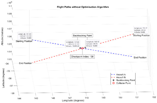
Figure 3.
Overview of flight paths for two leader aircraft colliding with no optimisation algorithm.
Table 2 provides an overview of the results for the flight paths with no optimisation algorithm, which did not incorporate any conflict avoidance measures.
Table 2.
Overview of results for flight paths without optimisation algorithm.
4.3. Scenario with Optimisation Algorithm
The optimised path simulations for Aircraft A and B, including conflict avoidance, are displayed below, presenting two scenarios labelled ‘Case I’ and ‘Case II’. To clearly convey the optimisation results, we have focused only on the conflict zone requiring optimisation, labelled as ‘Optimisation Start’ and ‘Optimisation End’ Figure 4, Figure 5, Figure 6 and Figure 7.
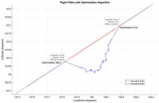
Figure 4.
Case I horizontal flight path display with optimisation algorithm.
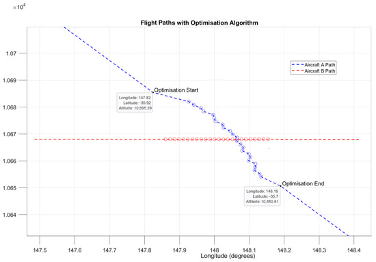
Figure 5.
Case I vertical flight path display with optimisation algorithm.
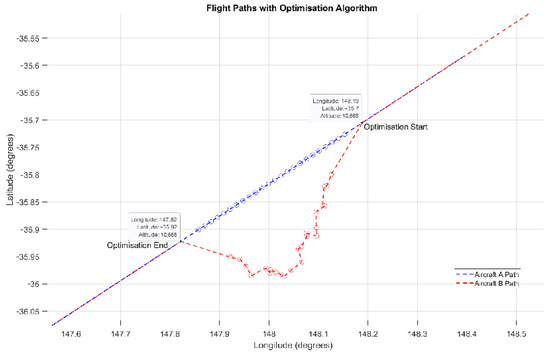
Figure 6.
Case II horizontal flight path display with optimisation algorithm.

Figure 7.
Case II vertical flight path display with optimisation algorithm.
Figure 4 displays the horizontal view (longitude vs. latitude) view of the Case I optimisation. In Case I, Aircraft B maintains its original flight path, while Aircraft A resolves the conflict; Figure 5 offers a vertical perspective (longitude vs. altitude) of Case I.
Figure 6 displays the horizontal view (longitude vs. latitude) view of the Case II optimisation. In Case II, Aircraft A maintains its original flight path, while Aircraft B resolves the conflict; Figure 7 offers a vertical perspective (longitude vs. altitude) of Case II. Both scenarios successfully eliminate potential path conflicts, with Case II offering a smoother flight path and demonstrating more effective optimisation. The Case II optimisation will be utilised to compare the results between non-formation and formation flights.
In both the Case I and Case II scenarios, the proposed method successfully detects and resolves the conflict. The optimisation results of each case are shown in Table 3 and Table 4. Compared to the flight path with no optimisation algorithm shown in Figure 3 with the results in Table 2, Case I optimisation resulted in a 1.13% increase in fuel consumption, a 0.66% increase in flight distance, and an 8.12% reduction in flight time. Case II optimisation showed a smaller increase in fuel consumption and flight distance, at 0.82% and 0.35%, respectively, and an 8.33% reduction in flight time. These results indicate that Case II is more efficient than Case I in terms of fuel consumption, time, and flight distance.
Table 3.
Results of Case I optimisation, Aircraft A adjusts, B stays en route, and conflict is avoided.
Table 4.
Results of Case II optimisation, Aircraft B adjusts, A stays en route, and conflict is avoided.
4.4. Increased Safety Redundancy
In the context of formation flight, increased safety redundancy is essential to ensure safe and effective operations in formation flight. Based on Australian separation standards, the initial horizontal separation distance is set to 9260 m to account for potential conflicts and enhance safety; this distance will be increased by 5% up to 20% for the non-formation and formation flight fuel analyses. As the current literature does not provide concrete guidelines or empirical data on the exact extent of this safety redundancy increase, these values are based on theoretical estimates rather than established practice.
4.5. Non-Formation Flight Fuel Analysis
To assess the total fuel consumption in a non-formation flight scenario for comparison to a formation flight, an assumption is made that a second aircraft is following Aircraft A and B in the simulation and exhibiting the same behaviour in terms of fuel consumption, flight time, and distance; however, they are not in a formation. Table 5, Table 6, Table 7, Table 8 and Table 9 below display the results in a non-formation flight scenario utilising the results of Case II using the optimisation algorithm for conflict avoidance.
Table 5.
Non-formation flight optimisation results with 9260 m safety redundancy.
Table 6.
Non-formation flight optimisation results with 9723 m safety redundancy.
Table 7.
Non-formation flight optimisation results with 10,186 m safety redundancy.
Table 8.
Non-formation flight optimisation results with 10,649 m safety redundancy.
Table 9.
Non-formation flight optimisation results with 11,112 m safety redundancy.
4.6. Formation Flight Fuel Analysis
As the follower aircraft in the formation is assumed to exhibit the same behaviour as the leader aircraft in fuel consumption, flight distance, and flight time, a conservative fuel efficiency improvement of 5% is applied to the follower based on the current literature. The fuel consumption of both the leader and follower aircraft for each safety redundancy value is shown below in Table 10, Table 11, Table 12, Table 13 and Table 14, with the total fuel consumption displayed.
Table 10.
Formation flight’s fuel consumption optimisation results with 9260 m safety redundancy.
Table 11.
Formation flight’s fuel consumption optimisation results with 9723 m safety redundancy.
Table 12.
Formation flight’s fuel consumption optimisation results with 10,186 m safety redundancy.
Table 13.
Formation flight’s fuel consumption optimisation results with 10,649 m safety redundancy.
Table 14.
Formation flight’s fuel consumption optimisation results with 11,112 m safety redundancy.
4.7. Comparison of Fuel Consumption Between Non-Formation and Formation Flight
Table 15 below compares the fuel consumption results of aircraft in non-formation and formation flights. The results indicate a 2.49–2.65% decrease in the total fuel consumption for aircraft in formation under Case II optimisation, incorporating conflict avoidance measures. The reduction in fuel is achieved despite the inclusion of increased safety redundancy values that enhance operational safety. These findings highlight the viability of formation flight as a practical approach for optimising fuel efficiency and resolving flight path conflicts, underscoring its potential benefits for enhancing aviation sustainability and operational performance on busy short-haul routes.
Table 15.
Comparison of the non-formation flight optimisation results with the formation flight optimisation results.
5. Discussion and Conclusions
This study successfully demonstrated the potential of formation flight to optimise fuel efficiency and resolve flight path conflicts on the busy Melbourne to Sydney route. Using a virtual conflict scenario in MATLAB 2023b, the proposed framework and algorithm effectively eliminated path conflicts and optimised fuel consumption with increased safety redundancy values. By utilising the more efficient Case II optimisation scenario, the study compared fuel consumption between non-formation and formation flights.
With an increased safety redundancy and a conservative 5% fuel efficiency improvement for the follower aircraft, the total fuel consumption has decreased from 2.49–2.65% for a two-aircraft formation flight as compared to a non-formation flight. These findings support the feasibility and benefits of formation flight in enhancing fuel efficiency and operational performance on busy routes, contributing to aviation sustainability.
Future research aims to extend the current study by exploring the application of formation flight principles to a wider range of flight routes. Investigating the impacts of bad weather conditions, air traffic density, and differing aircraft performance characteristics will provide a more comprehensive understanding of the feasibility of formation flight in Australian airspace. Further to this, a significant research gap exists in determining the precise safety redundancy requirements for formation, specifically concerning the optimal increase in separation distances.
Author Contributions
Conceptualization, O.C., M.L. and Y.X.; methodology, O.C., M.L. and Y.X.; software, O.C. and Y.X.; validation, O.C., C.B., M.L. and Y.X.; formal analysis, O.C., C.B., M.L. and Y.X.; investigation, O.C., C.B., M.L. and Y.X.; resources, O.C., C.B., M.L. and Y.X.; data curation, O.C. and Y.X.; writing—original draft preparation, O.C. and Y.X.; writing—review and editing, O.C., C.B., M.L. and Y.X.; visualization, O.C. and Y.X.; supervision, C.B. and M.L.; project administration, O.C., C.B., M.L. and Y.X. All authors have read and agreed to the published version of the manuscript.
Funding
This research received no external funding.
Institutional Review Board Statement
Not applicable.
Informed Consent Statement
Not applicable.
Data Availability Statement
Data are contained within the article.
Conflicts of Interest
The authors declare no conflicts of interest.
References
- Fleming, G.G.; de Lépinay, I.; Schaufele, R. Environmental Trends in Aviation to 2050; International Civil Aviation Organization: Montréal, QC, Canada, 2023; Available online: https://www.icao.int/environmental-protection/Pages/Environmental-Trends.aspx (accessed on 5 August 2024).
- Bureau of Infrastructure and Transport Research Economics. Australian Aviation Forecasts—2024 to 2050 (Research Report 157); Department of Infrastructure, Transport, Cities, Regional Development, Communications and the Arts: Canberra, Australia, 2024. Available online: https://www.bitre.gov.au (accessed on 5 August 2024).
- Department of Infrastructure, Transport, Regional Development, Communications and the Arts. Draft National Air Navigation Plan 2024–27; Department of Infrastructure, Transport, Regional Development, Communications and the Arts: Canberra, Australia, 2024. [Google Scholar]
- Airservices Australia. Australian Aviation Network Overview; Department of Infrastructure, Transport, Regional Development, Communications and the Arts: Canberra, Australia, 2024. [Google Scholar]
- Airservices Australia. Network Management: Balancing Demand and Capacity of Australia’s Aviation Network. 2024. Available online: https://www.airservicesaustralia.com/wp-content/uploads/Ground-Delay-Program-Factsheet-.pdf (accessed on 5 August 2024).
- Airservices Australia. Air Traffic Flow Management (ATFM) Pilot Briefing Paper, Version 5; Airservices Australia: Canberra, Australia, 2016; Available online: http://www.airservicesaustralia.com/services/air-traffic-flow-management/ (accessed on 5 August 2024).
- Bureau of Infrastructure and Transport Research Economics. International Airline Activity-May 2022 (Statistical Report); Department of Infrastructure, Transport, Regional Development, Communications and the Arts: Canberra, Australia, 2022. [Google Scholar]
- Bureau of Infrastructure and Transport Research Economics. Airline On Time Performance, 2023 Calendar Year Report; Department of Infrastructure, Transport, Regional Development, Communications and the Arts: Canberra, Australia, 2023. Available online: https://www.bitre.gov.au/statistics/aviation/otp_annual (accessed on 5 August 2024).
- Buckingham-Jones, S. Melbourne-Sydney Among World’s Busiest Flight Paths in 2023. The Australian Financial Review, 29 December 2023. Available online: https://www.afr.com/companies/transport/melbourne-sydney-among-world-s-busiest-flight-paths-in-2023-20231229-p5eu4q (accessed on 5 August 2024).
- Advisory Council for Aeronautics Research in Europe (ACARE). Beyond Vision 2020 (Towards 2050); European Commission, Directorate-General for Research: Brussels, Belgium, 2010. [Google Scholar]
- Weimerskirch, H.; Martin, J.; Clerquin, Y.; Alexandre, P.; Jiraskova, S. Energy saving in flight formation. Nature 2001, 413, 697–698. [Google Scholar] [CrossRef] [PubMed]
- Blake, W.B.; Bieniawski, S.R.; Flanzer, T.C. Surfing aircraft vortices for energy. J. Def. Model. Simul. Appl. Methodol. Technol. 2015, 12, 31–39. [Google Scholar] [CrossRef]
- Economon, T. Effects of wake vortices on commercial aircraft. In Proceedings of the 46th AIAA Aerospace Sciences Meeting and Exhibit, Reno, NV, USA, 7–10 January 2008. [Google Scholar] [CrossRef]
- Xu, J.; Ning, S.A.; Bower, G.; Kroo, I. Aircraft route optimization for formation flight. J. Aircr. 2014, 51, 490–501. [Google Scholar] [CrossRef]
- Bower, G.C.; Flanzer, T.C.; Kroo, I.M. Formation geometries and route optimization for commercial formation flight. In Proceedings of the 27th AIAA Applied Aerodynamics Conference, San Antonio, TX, USA, 22–25 June 2009. [Google Scholar] [CrossRef]
- Pol, S.; Houchens, B.C.; Marian, D.V.; Westergaard, C.H. Performance of AeroMINEs for Distributed Wind Energy. Presented at the AIAA SciTech, Orlando, CA, USA, 6–10 January 2020. [Google Scholar] [CrossRef]
- Kent, T.E.; Richards, A.G. Analytic approach to optimal routing for commercial formation flight. J. Guid. Control Dyn. 2015, 38, 1872–1882. [Google Scholar] [CrossRef]
- Dahlmann, K.; Matthes, S.; Yamashita, H.; Unterstrasser, S.; Grewe, V.; Marks, T. Assessing the climate impact of formation flights. Aerospace 2020, 7, 172. [Google Scholar] [CrossRef]
- Ball, M.O.; Hoffman, R.; Odoni, A.R.; Rifkin, R. A stochastic integer program with dual network structure and its application to the ground-holding problem. Oper. Res. 2003, 51, 167–171. [Google Scholar] [CrossRef]
- Mukherjee, A.; Hansen, M. A dynamic stochastic model for the single airport ground holding problem. Transp. Sci. 2007, 41, 444–456. [Google Scholar] [CrossRef]
- Kuhn, K.D. Ground delay program planning: Delay, equity, and computational complexity. Transp. Res. Part C Emerg. Technol. 2013, 35, 193–203. [Google Scholar] [CrossRef]
- Hummel, D. The Use of Aircraft Wakes to Achieve Power Reductions in Formation Flight. AGARD Conference Proceedings 584. 1996. Available online: https://apps.dtic.mil/sti/tr/pdf/ADA320134.pdf (accessed on 5 August 2024).
- Wagner, E.; Jacques, D.; Blake, W.; Pachter, M. Flight test results of close formation flight for fuel savings. In AIAA Atmospheric Flight Mechanics Conference and Exhibit; American Institute of Aeronautics and Astronautics: Reston, VA, USA, 2002. [Google Scholar] [CrossRef]
- Vachon, M.J.; Ray, R.J.; Walsh, K.R.; Ennix, K. F/A-18 aircraft performance benefits measured during the Autonomous Formation Flight Project. In AIAA Atmospheric Flight Mechanics Conference and Exhibit; American Institute of Aeronautics and Astronautics: Reston, VA, USA, 2002. [Google Scholar] [CrossRef]
- Pahle, J.; Berger, D.; Venti, M.; Faber, J.J.; Duggan, C.; Cardinal, K. An initial flight investigation of formation flight for drag reduction on the C-17 aircraft. In AIAA Atmospheric Flight Mechanics Conference and Exhibit; American Institute of Aeronautics and Astronautics: Reston, VA, USA, 2012. [Google Scholar] [CrossRef]
- Bieniawski, S.R.; Clark, R.W.; Rosenzweig, S.E.; Blake, W.B. Summary of flight testing and results for the formation flight for aerodynamic benefit program. In Proceedings of the AIAA SciTech 52nd Aerospace Sciences Meeting, National Harbor, MD, USA, 13–17 January 2014; American Institute of Aeronautics and Astronautics: Reston, VA, USA, 2014. [Google Scholar] [CrossRef]
- Lissaman, P.B.S.; Shollenberger, C.A. Formation flight of birds. Science 1970, 168, 1003–1005. [Google Scholar] [CrossRef] [PubMed]
- Hummel, D. Aerodynamic aspects of formation flight in birds. J. Theor. Biol. 1983, 104, 321–347. [Google Scholar] [CrossRef]
- Blake, W.; Multhopp, D. Design, performance and modeling considerations for close formation flight. In Proceedings of the 23rd AIAA Atmospheric Flight Mechanics Conference, Boston, MA, USA, 10–12 August 1998; American Institute of Aeronautics and Astronautics: Reston, VA, USA, 1998. AIAA Paper 1998-4343. Available online: https://www.ocw.mit.edu/courses/16-886-air-transportation-systems-architecting-spring-2004/ab208a8f2d9631cd6acb5f2d8e29d713_01_blakemulthopp.pdf (accessed on 5 August 2024).
- Frazier, J.W.; Gopalarathnam, A. Optimum downwash behind wings in formation flight. J. Aircr. 2003, 40, 799–803. [Google Scholar] [CrossRef]
- Ray, R.J.; Cobleigh, B.R.; Vachon, M.J.; John, C.S. Flight Test Techniques Used to Evaluate Performance Benefits During Formation Flight. NASA TP-2002-210730. 2002. Available online: https://arc.aiaa.org/doi/10.2514/6.2002-4492 (accessed on 5 August 2024).
- Pahle, J.; Berger, D.; Venti, M.; Faber, J.J.; Duggan, C.; Cardinal, K. A preliminary flight investigation of formation flight for drag reduction on the C-17 aircraft. In Proceedings of the AIAA Atmospheric Flight Mechanics Conference, Minneapolis, MN, USA, 13–16 August 2012; American Institute of Aeronautics and Astronautics: Reston, VA, USA, 2012; pp. 1–14. [Google Scholar]
- Voskuijl, M. Cruise range in formation flight. J. Aircr. Devoted Aeronaut. Sci. Technol. 2017, 54, 2184–2191. [Google Scholar] [CrossRef]


Disclaimer/Publisher’s Note: The statements, opinions and data contained in all publications are solely those of the individual author(s) and contributor(s) and not of MDPI and/or the editor(s). MDPI and/or the editor(s) disclaim responsibility for any injury to people or property resulting from any ideas, methods, instructions or products referred to in the content. |
© 2025 by the authors. Licensee MDPI, Basel, Switzerland. This article is an open access article distributed under the terms and conditions of the Creative Commons Attribution (CC BY) license (https://creativecommons.org/licenses/by/4.0/).