Does AutoML Outperform Naive Forecasting? ^†

Abstract

The availability of massive amounts of temporal data opens new perspectives of knowledge extraction and automated decision making for companies and practitioners. However, learning forecasting models from data requires a knowledgeable data science or machine learning (ML) background and expertise, which is not always available to end-users. This gap fosters a growing demand for frameworks automating the ML pipeline and ensuring broader access to the general public. Automatic machine learning (AutoML) provides solutions to build and validate machine learning pipelines minimizing the user intervention. Most of those pipelines have been validated in static supervised learning settings, while an extensive validation in time series prediction is still missing. This issue is particularly important in the forecasting community, where the relevance of machine learning approaches is still under debate. This paper assesses four existing AutoML frameworks (AutoGluon, H₂O, TPOT, Auto-sklearn) on a number of forecasting challenges (univariate and multivariate, single-step and multi-step ahead) by benchmarking them against simple and conventional forecasting strategies (e.g., naive and exponential smoothing). The obtained results highlight that AutoML approaches are not yet mature enough to address generic forecasting tasks once compared with faster yet more basic statistical forecasters. In particular, the tested AutoML configurations, on average, do not significantly outperform a Naive estimator. Those results, yet preliminary, should not be interpreted as a rejection of AutoML solutions in forecasting but as an encouragement to a more rigorous validation of their limits and perspectives.

1. Introduction

The pervasiveness of electronic devices enables the collection of temporal data (about production, development, sales) at a growing rate. Extracting actionable knowledge from temporal data requires specific technical skills, yet the growing availability of data is not accompanied by an equivalent increase in the number of experts able to analyze them, thus reducing their potential impact.

Automated machine learning (AutoML) [1] aims to fill this gap by automatizing the different phases of data analysis and providing suitable solutions for data scientists, practitioners and final users. AutoML approaches can help obtain a glimpse of knowledge about new data, for example, suggesting the optimal model to use. Data may also be too noisy or of poor quality, in which case AutoML would quickly reflect it, by showing failure in multiple pipelines, saving the data scientist a lot of time.

However, finding a procedure that automates the entire ML process for forecasting is a risky endeavor. Time series data have constraints and peculiarities (e.g., trend and seasonalities, outliers, drifts, abrupt changes) to handle in specific ways, often not compatible with more traditional tabular data. Furthermore, most AutoML approaches rely on the assumption that the higher the degree of search in the hyperparameter space, the better the final result. Now, in large dimensional and noisy settings, pushing the degree of grid search too far leads inevitably to a high degree of variance of the returned solution, which, if not adequately assessed with external validation data, could be prone to overfitting [2]. This is particularly the case of large dimensional settings like the ones that can be encountered in multivariate forecasting. In those cases, embedding, i.e., the transformation in a tabular form for supervised learning, produces high-dimensional input datasets. Automatizing the feature selection phase without accounting for an external validation set can be detrimental, returning over-optimistic assessment of the generalization accuracy of the chosen set of features.

Thus far, the main comparative studies on AutoML solutions are [3,4,5,6,7,8]. They generally compare various frameworks against each other on standard supervised learning tasks. Results show high variance [3], or no significant difference between models [7], although more recent comparisons appear to favor AutoGluon [8], suggesting the importance of feature preprocessing. However, frameworks tend not to significantly outperform traditional models (e.g., random forest within 4 h [4]) nor humans in easy classification tasks [5].

This paper assesses the capabilities of four AutoML frameworks (AutoGluon, H₂O, TPOT, Auto-sklearn) with respect to conventional statistical forecasting strategies (naive, exponential smoothing, Holt-Winter’s). This issue is particularly important in the forecasting community, where the relevance of machine learning approaches is still under debate [9]. In order to provide a fair comparison, we took advantages of the possibility provided by AutoML packages to limit the allowed computational time. The goal is to show experimentally the effectiveness of known AutoML frameworks on time series forecasting, challenging the framework by limiting their computational time and comparing the results with fast conventional forecasting strategies. In particular, the main contribution of this manuscript are:

• A description of several state-of-the-art AutoML frameworks;
• The comparison between several state-of-the-art AutoML frameworks on univariate and multivariate time series forecasting on different horizons;
• The assessment of their effectiveness against conventional forecasting strategies such as naive and exponential smoothing on comparable scale times.

Note that the constraint on the execution time is not simply an experimental decision but it reflects a criticism of the authors about the continuous increase of computing resources required by ML methods (notably deep learning). Since this resource consumption is not necessarily followed by a correspondent improvement of the overall performances, we think it is time for the forecasting community to investigate the trade-off between time (and energy) consumption vs. accuracy. The paper is organized as follows: Section 2 introduces the problem formulation, while Section 3 describes the adopted AutoML frameworks. The benchmarking experiments are described in Section 4, with the discussion and conclusions in Section 5.

2. Machine Learning and Forecasting

A multivariate and multitemporal model f aims at learning the mapping between past values and future values of an N-variate time series. Given a time resolution $\Delta t=t_i-t_{i-1}$ at time instant t, a lag L and a forecasting horizon h, the temporal dependency can be represented in the embedded form:

$$\left(\begin{array}{c}{y}_{1,t+1},\dots ,y_{1,t+h}\\ \cdots \\ y_{N,t+1},\dots ,y_{N,t+h}\end{array}\right)=f\left(\begin{array}{c}{y}_{1,t-L+1},\dots ,y_{1,t}\\ \cdots \\ y_{N,t-L+1},\dots ,y_{N,t}\end{array}\right)$$

(1)

The multi-input multi-output nature of (1) suggests the adoption of a multi-output approach (e.g., neural networks). However, since most learning algorithms available in AutoML frameworks are single-output, we will decompose the MIMO problem in a sequence of N multiple-input single-output (MISO) tasks:

$$\begin{array}{c}\left(\begin{array}{c}{y}_{1,t+1},\dots ,y_{1,t+h}\end{array}\right)=f_{1.1}\left(\begin{array}{c}{y}_{1,t-L+1},\dots ,y_{1,t}\\ \cdots \\ y_{N,t-L+1},\dots ,y_{N,t}\end{array}\right)\\ \cdots \\ \left(\begin{array}{c}{y}_{N,t+1},\dots ,y_{N,t+h}\end{array}\right)=f_{1.N}\left(\begin{array}{c}{y}_{1,t-L+1},\dots ,y_{1,t}\\ \cdots \\ y_{N,t-L+1},\dots ,y_{N,t}\end{array}\right)\end{array}$$

(2)

If we assume that there is no significant cross-series dependency, we may further decompose (2) into a set of N single-input, single-output (SISO) tasks:

$$\begin{array}{c}\left(y_{1,t+1},\dots ,y_{1,t+h}\right)=f_{2.1}\left(y_{1,t-L+1},\dots ,y_{1,t}\right)\\ \cdots \\ \left(y_{N,t+1},\dots ,y_{N,t+h}\right)=f_{2.N}\left(y_{N,t-L+1},\dots ,y_{N,t}\right)\end{array}$$

(3)

The above formulations make the natural adoption of supervised learning pipelines [10], which are typically composed of the following steps:

• Preprocessing: the observations are cleaned, normalized and rescaled. Missing data can be removed or replaced. New features may be produced by means of feature engineering [11].
• Dimensionality reduction: this step aims at reducing the input dimension, to diminish the computational burden and avoid numerical and statistical issues [12].
• Model estimation: this step estimates from the available data the input-output relationship.
• Performance assessment: the model performances are validated by means of a validation set, a subsample of the observed data that is kept aside to verify the ability of the model previously trained to correctly predict new unseen samples. This is followed by an analysis of the distribution of performance measures.

It is important to remark that those steps are either skipped or extremely simplified in conventional forecasting strategies (e.g., exponential smoothing) with an evident gain in terms of computational time.

2.1. Conventional Statistical Approaches

Those methods provide a quick insight to the behavior of a time series and are efficient to compute. The simplest approach is the naive: the time series forecast at time $t+1$ is provided by the last available observation at time t. Another simple technique is the mean model, where the forecast at time $t+1$ is the average of all previous observations up to time t. Exponential smoothing is an approach proposed by [13,14], based on exponentially decaying weighted averages of past observations. The approach favors recent observations, and its speed and reliability made it successful. A basic version is the simple exponential smoothing (4), suitable for data with no clear trend or seasonal pattern. $0\le \alpha \le 1$ is the smoothing parameter that controls the rate at which the weights decrease.

$${\widehat{y}}_{t+1\mid t}=\alpha y_t+\alpha (1-\alpha )y_{t-1}+\alpha {(1-\alpha )}^2{y}_{t-2}+\cdots$$

(4)

Holt and Winters [15] extended the method to capture trends and seasonality. The Holt-Winters seasonal method comprises the forecast equation and three smoothing equations (level, trend, seasonality). A corresponding multiplicative version exists [16]. When the seasonal variations are roughly constant, the additive method is preferred, and when the seasonal variations are changing proportional to the level of the series, the multiplicative method is chosen. By considering variations in the combinations of the trends and seasonal components, nine exponential smoothing methods are possible [17,18,19].

3. AutoML Frameworks

This section sketches the AutoML frameworks we selected for the experimental comparison. All of them provide the possibility to limit their execution time, enabling a fair comparison with faster statistical methods (Section 2.1).

H₂O is a distributed machine learning platform. Its AutoML module [20] covers a large selection of candidate models, including two stacked ensembles of all the trained models and of the best model of each family, respectively. It provides a simple and highly customizable interface where the user can specify the maximum time of the AutoML process or the maximum number of models to build in an AutoML run. The available ML algorithms are distributed random forest, including both random forest and extremely randomized trees; generalized linear models, XGBoost gradient boosting machine, H₂O gradient boosting machine, and deep neural network. Preprocessing is limited to automated target encoding of high dimension categorical variables.

Auto-sklearn [21] is a Python library for AutoML built on top of the scikit-learn library [22]. It uses 15 learners (notably k nearest neighbors, gradient boosting, stochastic gradient descent, random forest, AdaBoost), 14 feature preprocessing methods, and 4 data preprocessing methods. It leverages meta-learning by evaluating a set of meta-features (e.g., statistics about the number of data points, features) over hundreds of datasets and storing the most accurate related configurations. It also adopts Bayesian optimization to fit a probabilistic model to capture the relationship between hyperparameter settings and their measured performance. Additionally, it uses ensemble selection, a greedy procedure that, starting with an empty ensemble, iteratively adds the model that maximizes the ensemble effectiveness. Its data preprocessing includes one-hot encoding, imputation of missing values and normalization. Its feature preprocessing performs feature selection via principal component analysis, singular value decomposition and other methods.

AutoGluon [8] is a Python library for AutoML dealing with text, image, and tabular data. The set of learners includes neural networks, LightGBM boosted trees, CatBoost boosted trees, random forests, extremely randomized trees, and k nearest neighbors. Its preprocessing is split into model-agnostic preprocessing, including features categorization and treatment (e.g., encoding of categorical variables), and model-specific preprocessing applied on a copy of the data passed to each model. Multi-layer stack ensembling and repeated k-fold bagging are used to combine the base learners.

TPOT [23] is a tree-based pipeline optimization tool that automatically designs and optimizes ML pipelines using genetic programming (GP) [24]. It wraps the scikit-learn library [22], and offers the following models: decision tree, random forest, eXtreme gradient boosting, logistic regression and k nearest neighbor. The preprocessing and feature selection functionalities include standard scaler, randomized PCA, SelectKBest, and recursive feature elimination. Each ML pipeline is treated as a GP primitive, and GP trees are constructed from them. The process starts by generating 100 random tree-based pipelines and evaluating them, while for every generation, the top 20 are selected to maximize accuracy and minimize the number of operators. Each of the top 20 pipelines produces five copies with cross-overs or random mutations over the individual components of the pipeline. The whole procedure is repeated for 100 generations.

4. Experimental Benchmark

This section introduces the time series benchmarks, the methodology and the evaluation metrics and the results. We consider two public datasets made available in [25]. The format of the dataset has been adapted to ease research related to multivariate time series. A link can be found in the footnotes of Section 5.

• Electricity consumption: the original dataset (https://archive.ics.uci.edu/ml/datasets/ElectricityLoadDiagrams20112014, accessed on 30 March 2021) contains electricity consumption of 370 clients recorded every 15 min from 2011 to 2014. The preprocessed dataset contains hourly consumption (in kWh) of 321 clients from 2012 to 2014.
• Exchange rate: the dataset (possible source: https://fred.stlouisfed.org/series/EXUSEU, accessed on 3 March 2021) is a collection of the daily exchange rates of eight foreign countries, including Australia, Great Britain, Canada, Switzerland, China, Japan, New Zealand and Singapore. The considered time ranges from 1990 to 2016.

We benchmark four AutoML frameworks against simple and conventional forecasting strategies by adopting a SISO (3) approach for univariate forecasting and a MISO (2) approach for multivariate forecasting. The rationale behind the choice of MISO over MIMO (1) is that not all AutoML frameworks provide the possibility of predicting multiple-output, and this would not have produced a fair comparison. An additional reason is the intrinsic univariate nature of conventional methods such as naive or exponential smoothing: a MISO approach provides a more natural comparison by predicting only one variable. For the univariate case, we decide to work with the first available variable, without loss of generality. The choice of additional variables for the multivariate case is made as follows: starting from the first variable, we pick its N most correlated variables, and we forecast on the first variable.

Preprocessing: we do not perform any data preprocessing for three reasons. First, data are already in a format that does not need particular treatment. Second, some AutoML frameworks, as mentioned in Section 3, include some data preprocessing. If this improves the performances, the corresponding framework should be rewarded. Third, this work aims at benchmarking models, rather than maximizing the correctness of forecasting: as long as all models are provided with the same data, the benchmark is fair.

AutoML: the selected frameworks treat tabular data in a supervised learning setting. They hence require an embedding for the time series (see Section 1). The lag parameter for the embedding was fixed at $L=5$, and future work will explore other values. Since one of the two time series considered contained at most eight variables, we decided to set the possible number of variables to $v\in \left[1,3,5,8\right]$. The values for the horizon have been fixed to $h\in \left[1,2\right]$ and the time allowed for each AutoML framework was limited to t = [60 s, 120 s, 300 s]. These values are low with respect to standard AutoML times for an optimal exploration of the space of parameters, but the comparison with particularly fast methods requires those limitations. Longer time frames will be considered in future work. The combinations of all tested parameters are presented in (5), and one experiment has been carried out for each of them. No additional parameter has been set to the frameworks.

$$\left[\begin{array}{c}\mathrm{Auto}-\mathrm{sklearn}\hfill \\ \mathrm{AutoGluon}\hfill \\ {\mathrm{H}}_2\mathrm{O}\hfill \\ \mathrm{TPOT}\hfill \end{array}\right]\times \left[\begin{array}{c}1\mathrm{variable}\hfill \\ 3\mathrm{variables}\hfill \\ 5\mathrm{variables}\hfill \\ 8\mathrm{variables}\hfill \end{array}\right]\times \left[\begin{array}{c}\mathrm{Horizon}1\hfill \\ \mathrm{Horizon}2\hfill \end{array}\right]\times \left[\begin{array}{c}\mathrm{Time}60\mathrm{s}\hfill \\ \mathrm{Time}120\mathrm{s}\hfill \\ \mathrm{Time}300\mathrm{s}\hfill \end{array}\right]$$

(5)

Conventional forecasting strategies: we consider the naive predictor as our baseline, and from the exponential smoothing family, we choose the simple exponential smoothing and four variations of Holt-Winters. We focus on Holt-Winters because of its historical effectiveness in forecasting [15]. The mentioned variations are summarized in

Table 1. Exponential smoothing-approaches considered in this work, specifying the nature of their trends and seasonal components.

Method	Trend Comp.	Seasonal Comp.
Simple exponential smoothing	None	None
Additive Holt-Winters’ method	Additive	Additive
Multiplicative Holt-Winters’ method	Additive	Multiplicative
Additive Holt-Winters’ damped method	Additive damped	Additive
Multiplicative Holt-Winters’ damped method	Additive damped	Multiplicative

.

Train, validation and metrics: We consider the absolute error, i.e., the absolute difference between the real value $y_i$ and the predicted value ${\widehat{y}}_i$. Our validation strategy divides the time series into three equal fragments, considering one additional third at each iteration. The last 16 points of this set are considered as the validation set, while all the previous points are the train set. This results in a total of 48 test points from 3 different areas of the time series.

Experimental Results

Figure 1, Figure 2, Figure 3 and Figure 4 show critical distance plots, i.e., a graphical representation of the results of the Friedman statistical test (with post hoc Nemenyi test), as suggested in [26]. The methods are ordered according to their performance from left to right (left is better), while the black bar connects methods that are not significantly different (at $p=0.05$). The nomenclature chosen follows the pattern framework_variables_time. A selection of models is shown in Figure 1, Figure 2 and Figure 3; in particular, we plot the most and least performing variant for each AutoML framework and all the conventional methods. Figure 1 and Figure 2 present the methods ranking over the electricity and exchange time series, respectively, averaging over different horizons. Figure 3 represents the average over both time series. The same results of Figure 3 are presented in Figure 4, but the 20 most performing models are considered.

Table 2. Win/loss count with respect to the naive approach presented in Section 2.1. The counts are made over the four case studies considered: electricity and exchange time series for 1-step ahead and 2-steps ahead forecasting. The nomenclature chosen follows the pattern framework_variables_time, and the metric considered is the absolute error.

Model	Wins	Losses	Model	Wins	Losses
Holt-Winters (add${}_d$-add)	146	46	h2o_v3_300s	66	126
Holt-Winters (add-add)	146	46	autogluon_v3_300s	65	127
SimpleExpSmoothing	139	53	tpot_v3_60s	65	127
Holt-Winters (add${}_d$-mul)	138	54	h2o_v5_60s	65	127
Holt-Winters (add-mul)	138	54	h2o_v3_60s	63	129
h2o_v1_120s	80	112	h2o_v8_60s	62	130
h2o_v1_300s	79	113	tpot_v5_60s	62	130
autosklearn_v1_300s	75	117	autosklearn_v1_60s	61	131
h2o_v1_60s	75	117	tpot_v8_60s	60	132
h2o_v8_120s	74	118	autogluon_v5_300s	60	132
autogluon_v1_300s	74	118	tpot_v8_120s	60	132
tpot_v1_120s	74	118	autogluon_v8_300s	59	133
tpot_v8_300s	74	118	autogluon_v8_120s	59	133
autogluon_v1_60s	73	119	autogluon_v5_120s	59	133
tpot_v1_60s	72	120	autogluon_v8_60s	57	135
tpot_v1_300s	71	121	autogluon_v5_60s	53	139
h2o_v5_300s	69	123	autosklearn_v3_300s	51	141
autogluon_v1_120s	69	123	h2o_v5_120s	50	142
autogluon_v3_120s	69	123	autosklearn_v5_300s	36	156
h2o_v8_300s	68	124	autosklearn_v3_120s	18	174
tpot_v5_120s	67	125	autosklearn_v5_120s	17	175
autogluon_v3_60s	67	125	autosklearn_v5_60s	14	178
autosklearn_v1_120s	67	125	autosklearn_v8_300s	14	178
tpot_v5_300s	66	126	autosklearn_v8_60s	9	183
tpot_v3_300s	66	126	autosklearn_v8_120s	5	187
tpot_v3_120s	66	126	autosklearn_v3_60s	2	190
h2o_v3_120s	66	126	Naive	Base	Base

presents the win/losses of all studied approaches with respect to the naive predictor. In all cases, the metric considered is the absolute error. This analysis highlights the following results:

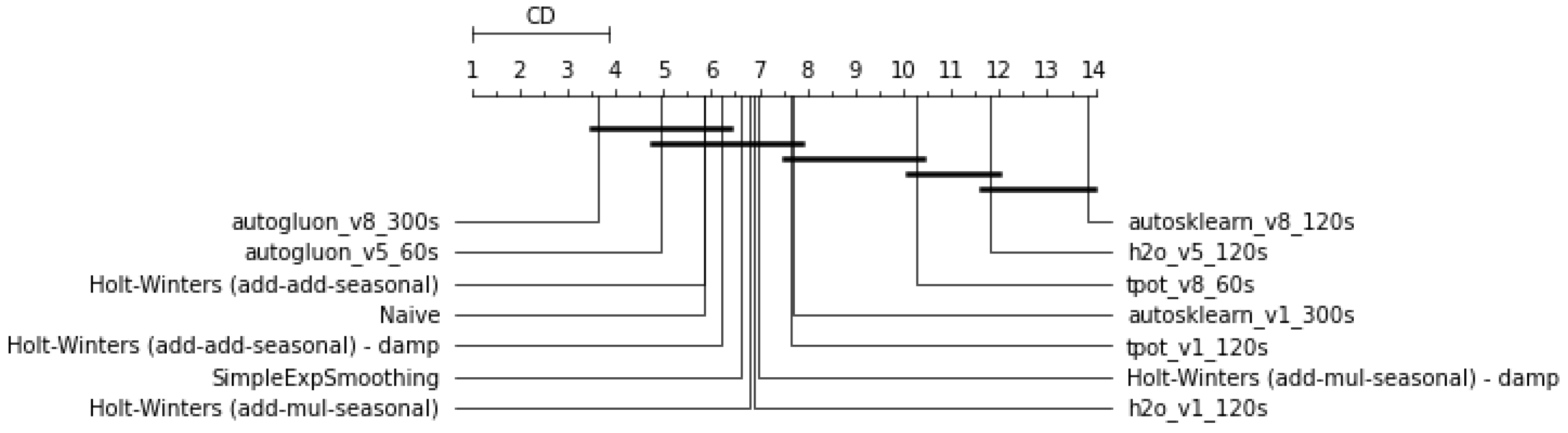
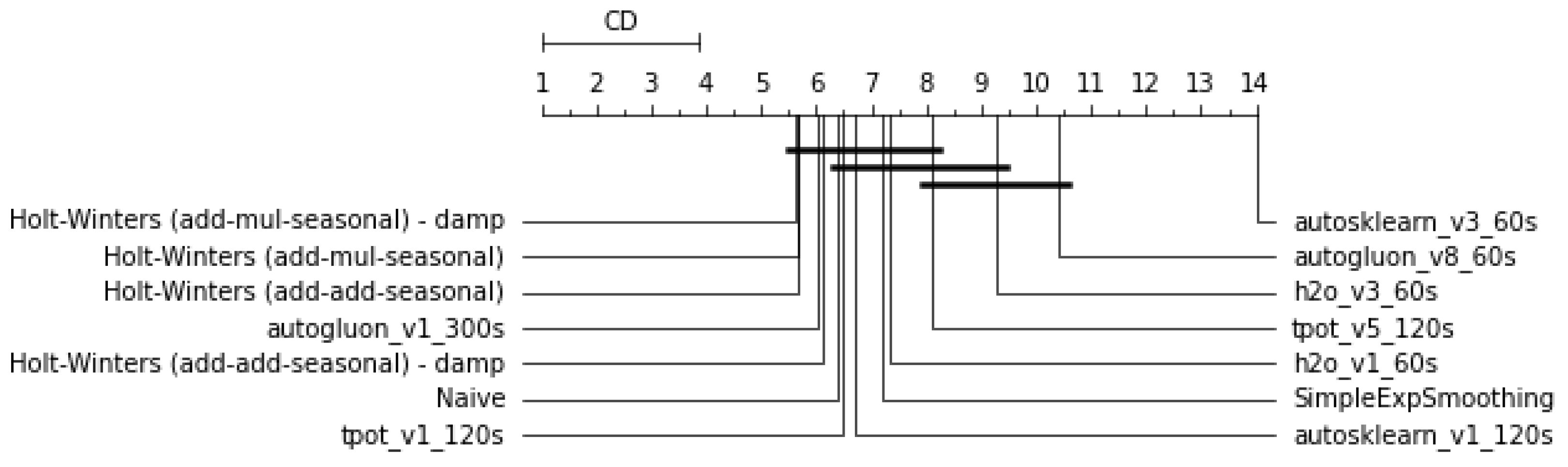
• Short-range training times (in the order of few minutes) are not sufficient for the AutoML frameworks considered to significantly outperform conventional methods (Figure 3). For short-horizons quick forecasting, it might therefore be convenient to rely on the latter.
• In terms of training time, 120 s seems to allow slightly better generalization ability than 60 or 300 s (Table 2). This might indicate that with 60 s, the models tend to underfit and with 300 s to overfit the observations.
• All traditional methods dominate every AutoML method in terms of wins count with respect to the naive (Table 2), which reflects the strong forecasting ability of the exponential smoothing family of methods. It could be appropriate to consider those methods as a baseline.
• Moving from a univariate SISO to multivariate MISO approach does not improve the performances of any method despite that the variables are added by maximizing correlation. This seems to suggest a lack of effectiveness in the feature selection approaches of the AutoML frameworks, when implemented.

5. Conclusions, Recommendations and Future Work

Automated machine learning is a promising research direction aiming to support practitioners in unleashing the potential of ML for data science. Various frameworks currently exist, and they differ by their feature selection, model selection and parameter optimization approaches. With sufficient time and resources, they have been showing excellent results in several learning problems.

This paper supports the idea that it is probably too soon to consider them as a full-fledged solution for time series forecasting. In particular, we deem that most solutions hang more on the complexity and comprehensiveness side than on the one of a rigorous validation of the added value with respect to simpler, yet less prone to overfitting, solutions. This is particularly delicate in forecasting settings where the high noise, the large dimension and the small number of samples would advise for a more cautious attitude with respect to complex automatic solutions. Our conclusion is supported by a benchmark of selected AutoML frameworks against simple statistical methods like naive and Holt-Winter’s. The obtained results suggest that, in the short term, AutoML frameworks do not significantly outperform traditional methods, and relying exclusively on them might not be the optimal solution.

On the basis of the results obtained, we would like to make some recommendations to the AutoML community. It is important that any automatic selection strategy is supported by an external validation dataset, including significance tests with respect to simple and naive strategies. In the case of limited data, permutation strategies may be adopted to assess the added value of complex ML pipelines, as well. Last but not least, we deem that AutoML tools should have a pedagogical role with respect to end users by educating them in terms of the trade-off between accuracy and computational resource (and energy) consumption. For instance, a graphical representation of the cost–benefit ratio could help in that sense.

Further work will assess the impact of longer computational time allowed to the AutoML models (in the order of hours or days) and repeat the tests for larger horizons, where traditional methods might suffer. AutoML frameworks also offer deep customization to improve their performance, which has not been considered in this work and will be studied. Additionally, an analysis of other frameworks that offer time-series-specific treatments is foreseen.

References

1. He, X.; Zhao, K.; Chu, X. AutoML: A Survey of the State-of-the-Art. Knowl. Based Syst. 2021, 212, 106622. [Google Scholar] [CrossRef]
2. Bontempi, G. A blocking strategy to improve gene selection for classification of gene expression data. IEEE/ACM Trans. Comput. Biol. Bioinform. 2007, 4, 293–300. [Google Scholar] [CrossRef] [PubMed]
3. Balaji, A.; Allen, A. Benchmarking automatic machine learning frameworks. arXiv 2018, arXiv:1808.06492. [Google Scholar]
4. Gijsbers, P.; LeDell, E.; Thomas, J.; Poirier, S.; Bischl, B.; Vanschoren, J. An open source automl benchmark. arXiv 2019, arXiv:1907.00909. [Google Scholar]
5. Hanussek, M.; Blohm, M.; Kintz, M. Can AutoML outperform humans? An evaluation on popular OpenML datasets using AutoML Benchmark. arXiv 2020, arXiv:2009.01564. [Google Scholar]
6. Guyon, I.; Sun-Hosoya, L.; Boullé, M.; Escalante, H.J.; Escalera, S.; Liu, Z.; Jajetic, D.; Ray, B.; Saeed, M.; Sebag, M.; et al. Analysis of the AutoML Challenge Series 2015–2018. In Automated Machine Learning; Hutter, F., Kotthoff, L., Vanschoren, J., Eds.; The Springer Series on Challenges in Machine Learning; Springer: Cham, Switzerland, 2019. [Google Scholar] [CrossRef] [Green Version]
7. Zöller, M.A.; Huber, M.F. Benchmark and survey of automated machine learning frameworks. arXiv 2019, arXiv:1904.12054. [Google Scholar]
8. Erickson, N.; Mueller, J.; Shirkov, A.; Zhang, H.; Larroy, P.; Li, M.; Smola, A. Autogluon-tabular: Robust and accurate automl for structured data. arXiv 2020, arXiv:2003.06505. [Google Scholar]
9. Makridakis, S.; Spiliotis, E.; Assimakopoulos, V. Statistical and Machine Learning forecasting methods: Concerns and ways forward. PLoS ONE 2018, 13, e0194889. [Google Scholar] [CrossRef] [PubMed] [Green Version]
10. Bontempi, G.; Taieb, S.B.; Le Borgne, Y.A. Machine learning strategies for time series forecasting. In European Business Intelligence Summer School; Springer: Berlin, Germany, 2012; pp. 62–77. [Google Scholar]
11. Christ, M.; Braun, N.; Neuffer, J.; Kempa-Liehr, A.W. Time series feature extraction on basis of scalable hypothesis tests (tsfresh—A python package). Neurocomputing 2018, 307, 72–77. [Google Scholar] [CrossRef]
12. Bermingham, M.L.; Pong-Wong, R.; Spiliopoulou, A.; Hayward, C.; Rudan, I.; Campbell, H.; Wright, A.F.; Wilson, J.F.; Agakov, F.; Navarro, P.; et al. Application of high-dimensional feature selection: Evaluation for genomic prediction in man. Sci. Rep. 2015, 5, 1–12. [Google Scholar] [CrossRef] [PubMed] [Green Version]
13. Brown, R.G. Statistical Forecasting for Inventory Control; McGraw/Hill: New York, NY, USA, 1959. [Google Scholar]
14. Holt, C.C. Forecasting seasonals and trends by exponentially weighted moving averages. Int. J. Forecast. 2004, 20, 5–10. [Google Scholar] [CrossRef]
15. Goodwin, P. The holt-winters approach to exponential smoothing: 50 years old and going strong. Foresight 2010, 19, 30–33. [Google Scholar]
16. Hyndman, R.; Koehler, A.B.; Ord, J.K.; Snyder, R.D. Forecasting with Exponential Smoothing: The State Space Approach; Springer Science & Business Media: Berlin/Heidelberg, Germany, 2008. [Google Scholar]
17. Pegels, C.C. Exponential forecasting: Some new variations. Manag. Sci. 1969, 15, 311–315. [Google Scholar]
18. Gardner, E.S., Jr. Exponential smoothing: The state of the art. J. Forecast. 1985, 4, 1–28. [Google Scholar] [CrossRef]
19. Taylor, J.W. Exponential smoothing with a damped multiplicative trend. Int. J. Forecast. 2003, 19, 715–725. [Google Scholar] [CrossRef] [Green Version]
20. LeDell, E.; Poirier, S. H2O AutoML: Scalable Automatic Machine Learning. In Proceedings of the 7th ICML Workshop on Automated Machine Learning (AutoML), Online, 18 July 2020. [Google Scholar]
21. Feurer, M.; Klein, A.; Eggensperger, K.; Springenberg, J.; Blum, M.; Hutter, F. Efficient and Robust Automated Machine Learning. 2015. Available online: http://papers.nips.cc/paper/5872-efficient-and-robust-automated-machine-learning (accessed on 30 March 2021).
22. Pedregosa, F.; Varoquaux, G.; Gramfort, A.; Michel, V.; Thirion, B.; Grisel, O.; Blondel, M.; Prettenhofer, P.; Weiss, R.; Dubourg, V.; et al. Scikit-learn: Machine Learning in Python. CoRR 2012, abs/1201.0490. [Google Scholar]
23. Olson, R.S.; Bartley, N.; Urbanowicz, R.J.; Moore, J.H. Evaluation of a Tree-based Pipeline Optimization Tool for Automating Data Science. In Proceedings of the Genetic and Evolutionary Computation Conference (GECCO ’16), Denver, CO, USA, 20–24 July 2016; ACM: New York, NY, USA, 2016; pp. 485–492. [Google Scholar] [CrossRef] [Green Version]
24. Banzhaf, W.; Nordin, P.; Keller, R.E.; Francone, F.D. Genetic Programming: An Introduction; Morgan Kaufmann Publishers: San Francisco, CA, USA, 1998; Volume 1. [Google Scholar]
25. Lai, G.; Chang, W.C.; Yang, Y.; Liu, H. Modeling long-and short-term temporal patterns with deep neural networks. In Proceedings of the 41st International ACM SIGIR Conference on Research & Development in Information Retrieval, Ann Arbor, MI, USA, 8–12 July 2018; pp. 95–104. [Google Scholar]
26. Demšar, J. Statistical comparisons of classifiers over multiple data sets. J. Mach. Learn. Res. 2006, 7, 1–30. [Google Scholar]
Figure 1. CD plot—selected models comparison of the absolute errors over the validation set for the electricity time series.
Engproc 05 00036 g001
Figure 2. CD plot—selected models comparison of the absolute errors over validation set for the exchange time series.
Engproc 05 00036 g002
Figure 3. CD plot—selected models comparison of the absolute errors over validation set for both time series.
Engproc 05 00036 g003
Figure 4. CD plot—top 20 models comparison of the absolute errors over validation set for both time series.
Engproc 05 00036 g004