Abstract
The rapid emergence of the 5G networks has posed a number of new planning problems, which should be carefully analyzed to optimize the installation of the new technologies and to integrate them into the existing mobile network. The main planning objectives are to build up a network satisfying the expected traffic demands in its various sections, in compliance with the performance quality targets suggested by international committees International Telecommunication Union (ITU), Comité Consultatif International pour la Radio (CCIR), etc. The following paper discusses some of the main aspects which should be evaluated in the planning stage of 5G radio relay transmission, such as traffic capacity, propagation problems, and interference problems.
1. Introduction
New technologies for transmitting and receiving signals play a leading role in the basis of key decisions in the development of radio relay networks. As the main direction in the development of the physical basis of such networks in [1], the unconditional use of intelligent (digital) antenna arrays and the use of MIMO (Multiple Input Multiple Output) technology is noted. Among the possibilities provided by the technology of digital antenna arrays (DA), it should be noted, that the adaptive control of the orientation of the partial beam maxima, which allows focusing of the signal energy in certain directions (toward the receiving device), contributing to increasing the signal-to-noise ratio. The narrow antenna beam also reduces interference, improves the signal-to-noise ratio, and thus increases the efficiency of the use of the signal power spectrum. With the growth of IoT, this method finds application in various communication systems such as contemporary mobile communications 4G (LTE), 5G, WCDMA, 6LoWPAN, etc. [1,2].
Operating conditions of various radio technical systems (RTS), as a rule, are characterized by a complex interference environment, which significantly reduces the quality of detection and filtering of useful signals. One of the main areas of theory and technology for dealing with passive and active disturbances is their compensation. In [3], a method for the distribution of telecommunication traffic with optimal usage of the available bandwidth was proposed.
The clearest principle of interference compensation is based on a two-channel reception method, when there is a useful signal and interference in the main channel and the presence of interference in the compensation channel, the useful signal is significantly weakened.
Adding the main and offset channel signals in the antiphase results in a reduction in the noise level without significant signal attenuation. Such an interference suppression approach has given good results in evaluating system performance and Quality of Service in 5G networks [4], in communication systems [5], and in increasing the accuracy of interference reproduction and, therefore, the application of its high-quality compensation is achieved by increasing the number of auxiliary channels. The possibility of generalizing this method in the case of multi-channel radio reception appeared as a result of the development of antenna arrays, the antenna patterns of which are adapted to the spatial location of radio emission sources.
In addition to the classical use of orthogonal frequency division multiplexing (OFDM) in MIMO systems, in recent years the use of high-performance multilevel modulations 1024QAM, 2048QAM (the numbers indicate the number of symbol levels used to modulate complex signal amplitudes) and XPIC MIMO technology with dual polarization to increase channel capacity [6].
2. Use of Polarization Multiplexing
This technology makes it possible to double the data rate without expanding the signal bandwidth. The increase in transmission speed is achieved by creating two transmitter streams operating in the same band but at orthogonal polarizations (vertical and horizontal).
Since for the application of high levels of QAM modulation it is necessary to ensure a low level of cross-polarization interference, in the case of OFDM signals this problem can be solved within two main methods of frequency distribution of the subcarriers of the dual polarization signals.
The ACDP (Adjacent Channel Dual Polarized) method involves the use of different signal frequencies (adjacent or adjacent in the frequency network) in orthogonal polarizations. Therefore, its practical implementation is simpler from a technical and algorithmic point of view, and the decoupling between signals with different polarizations is further increased due to the frequency-selective action of the amplitude-frequency characteristics of the frequency filters. However, with the OFDM signal modulation, the ACDP method does not allow efficient use of the allocated spectral range.
This drawback is removed by the method of increasing the throughput in radio relay systems by using polarization decoupling in one (combined) frequency channel (Co-channel Dual Polar system—CCDP). It has been known for a long time and is actively used by manufacturers of base radio relay systems and intra-area radio relay lines.
2.1. Cross-Polarization Interference Cancellation
The efficiency of CCDP implementation is largely determined by the cross-polarization decoupling (XPD) coefficient of the antennas. The problem of minimizing cross-polarization interference in the CCDP method can be successfully solved by introducing a special Cross-Polarization Interference Cancellation (XPIC) system in the equipment.
When the signal passes through the propagation channel, it is depolarized [7], as a result of which the orthogonality is violated, which leads to the need to supplement the communication system with polarization compensation devices. XPIC technology allows compensating for the negative influence of the “adjacent” signal and increases the level of signal isolation in the receiver [6].
In the transmission part of the system, two data streams are formed, and both streams are transferred to the carrier frequency, after which the signals enter the antenna, one with horizontal and the other with vertical polarization. After passing through the propagation channel, the signals are received by the receiving antenna. The separation of the signals is done according to the polarization characteristic, but during transmission over the communication channel, the signals are depolarized, thus, signals of both polarizations appear in each receiving path.
In the transmission part of the system, two data streams are formed, as both streams are transferred to the carrier frequency, after which the signals enter the antenna, one with horizontal and the other with vertical polarization. After passing through the propagation channel, the signals are received by the receiving antenna. The separation of the signals is done according to the polarization characteristic, but during transmission over the communication channel, the signals are depolarized, thus, signals of both polarizations appear in each receiving path based on the pilot signals, the Signal-to-Noise Ratio (SNR) power (adjacent polarization signal) is estimated and the weight coefficients of the filters are estimated. Compensating signals are formed at the output of the filters, which are added to the received signals to suppress SNR. As the level of cross-polarization changes, the filters adapt for maximum isolation level.
In the simplest embodiment, the essence of the XPIC procedure is that control signals applied sequentially to each of the orthogonal polarizations are used to first measure the levels of “penetration” of signals from the adjacent polarization channel. Assuming that the measured cross-polarization coupling coefficients do not change too dynamically, the obtained coefficients are used at the stage of receiving information messages to subtract the cross-polarization interference from the useful signals. In this case, the analytical record of the XPIC procedure can be represented as:
where , are the complex signal voltages obtained from the output of the r-th frequency filter in the channels of horizontal and vertical polarization as a result of the XPIC operation, are the complex voltages of the signals obtained from the output of the r-th frequency filter in the channels of the horizontal and the vertical polarization before performing the XPIC operation, and are the cross-polarization coupling coefficients measured at the link coupling stage [6].
A more rigorous approach involves the simultaneous application of two control signals on orthogonal polarizations. At the same time, by analogy, with the evaluation of signal transmission channels in MIMO systems, the characteristics of polarization channels are evaluated. Assuming that the two polarization channels have identical characteristics, that is, not only the equality of the cross-polarization coupling coefficients = is fulfilled but the transmission coefficients at the main polarizations ( = ) are also equal. Under such assumptions, it is needed to be solved a system of equations, such as:
where the unknowns are the coefficients () and (), and the quantities PVr PHr, are the known complex amplitudes of the control signals emitted at orthogonal polarizations.
According to [2], the use of XPIC in the carrier frequency range ≥ 18 GHz with 128QAM modulation makes it possible to use the same subcarrier frequency in both polarizations, which doubles the capacity of the communication channel.
2.2. Frequency Diversity
The idea of frequency diversity is related to the concept of the coherence band of the channel. This value characterizes the maximum width of the frequency interval in which the attenuation can be considered flat, i.e., the harmonic attenuation of the signal is almost 100% dependent. In this case, the attenuation of harmonics separated in frequency by an interval exceeding the coherence band is assumed to be independent. In other words, an additional transmission channel is arranged, duplicating the transmission of the signal at the main frequency and having a frequency shift sufficient to eliminate channel correlation.
3. Analysis and Discussion
All collected data from three characteristic traces were analyzed—Trace 1 (mountain above water surface—dam); Trace 2 (on the coast of the Black Sea as the line is above the sea surface); and Track 3 (flat terrain, away from water resources).
A mathematical model with adaptive filtration of the coefficients of the following type was synthesized:
where â(t) is the estimate of the predicted value at the moment t; a(t − i)—the current value at the moment k = t − i; wi—the weight factor at the moment i.
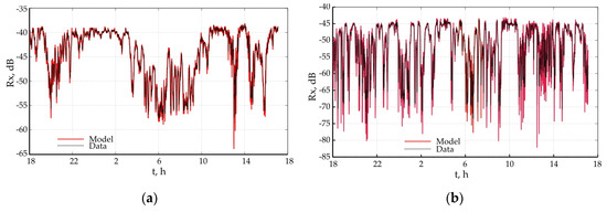
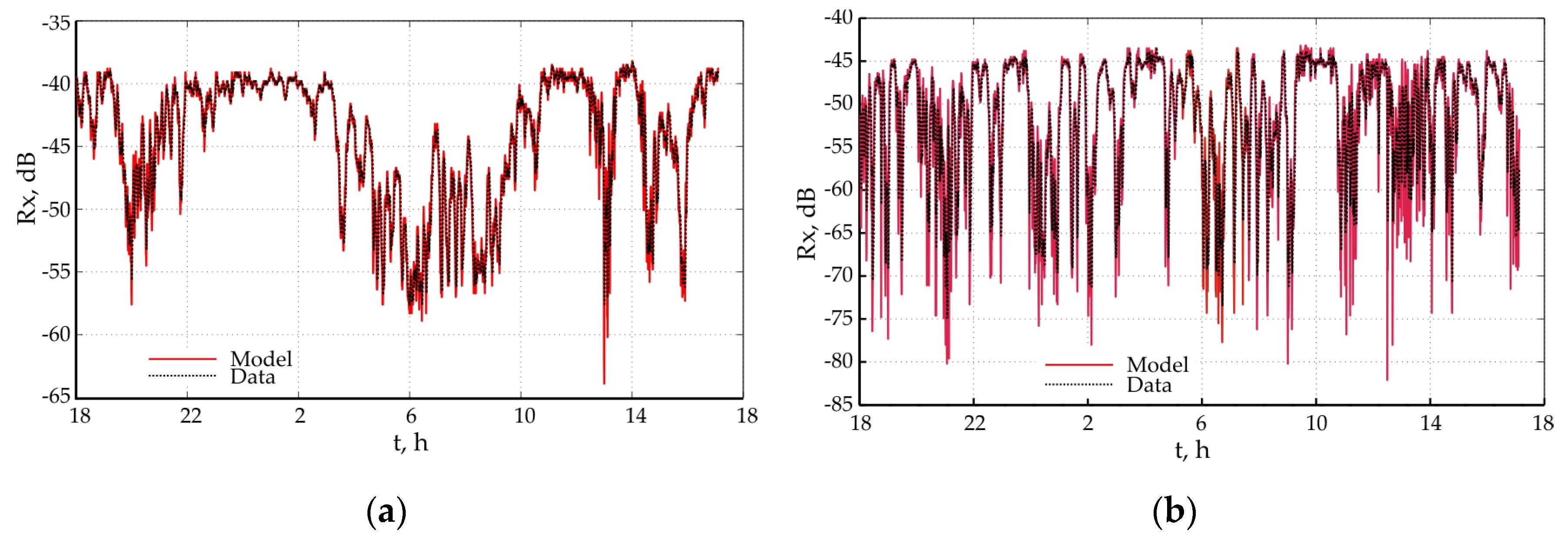
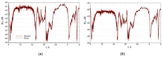
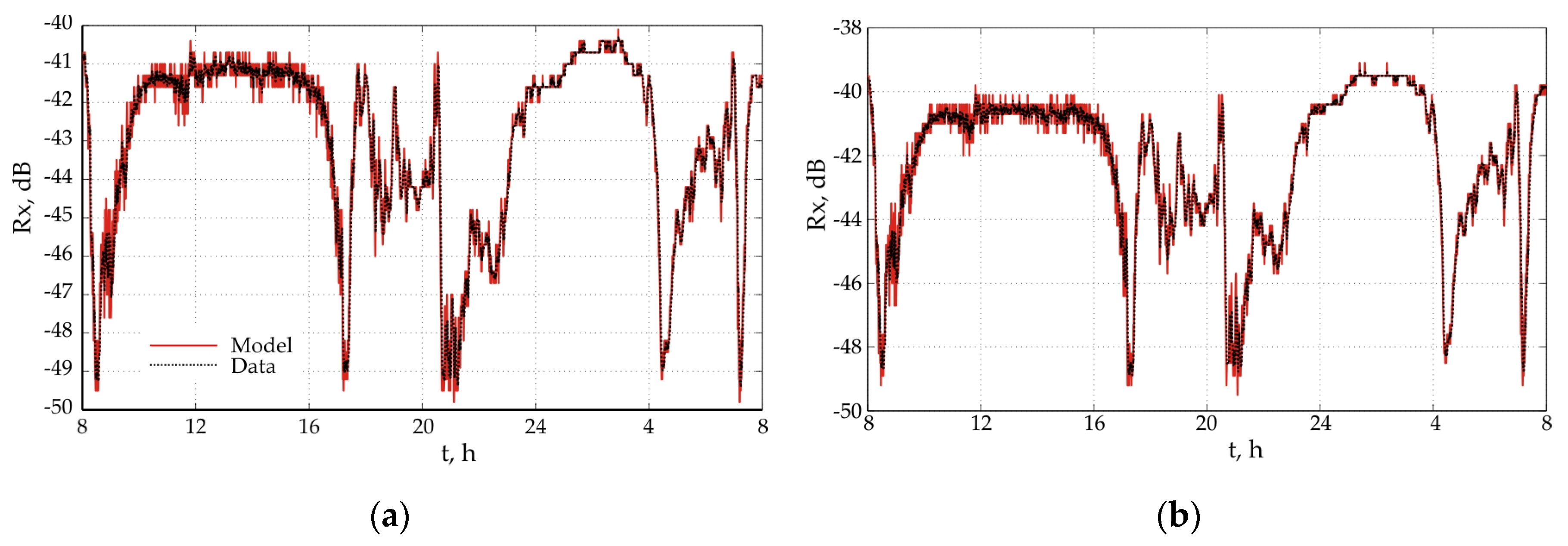
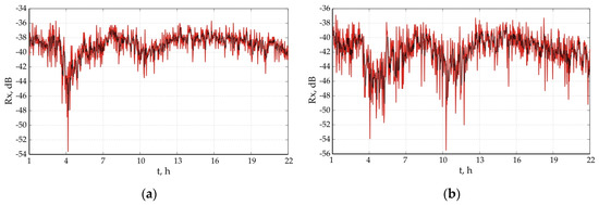
Figure 1, Figure 2 and Figure 3 show the correlations between the measured values in the signal levels (black line) and the theoretically determined by the model (blue line) for the three tracks. It can be seen that the match is very good as more significant differences between the measured and modeled values are observed in cases of fading.
Figure 1.
Simulated data of radio link Dospat—Saritsa: (a) 8 GHz; (b) 18 GHz.
Figure 2.
Simulated data of radio link Opan—Vasil Levski: (a) horizontal polarization; (b) vertical polarization.
Figure 3.
Simulated data of radio link Dyuni—St. Toma: (a) 18 GHz; (b) 28 GHz: red line is the model, black line is the data.
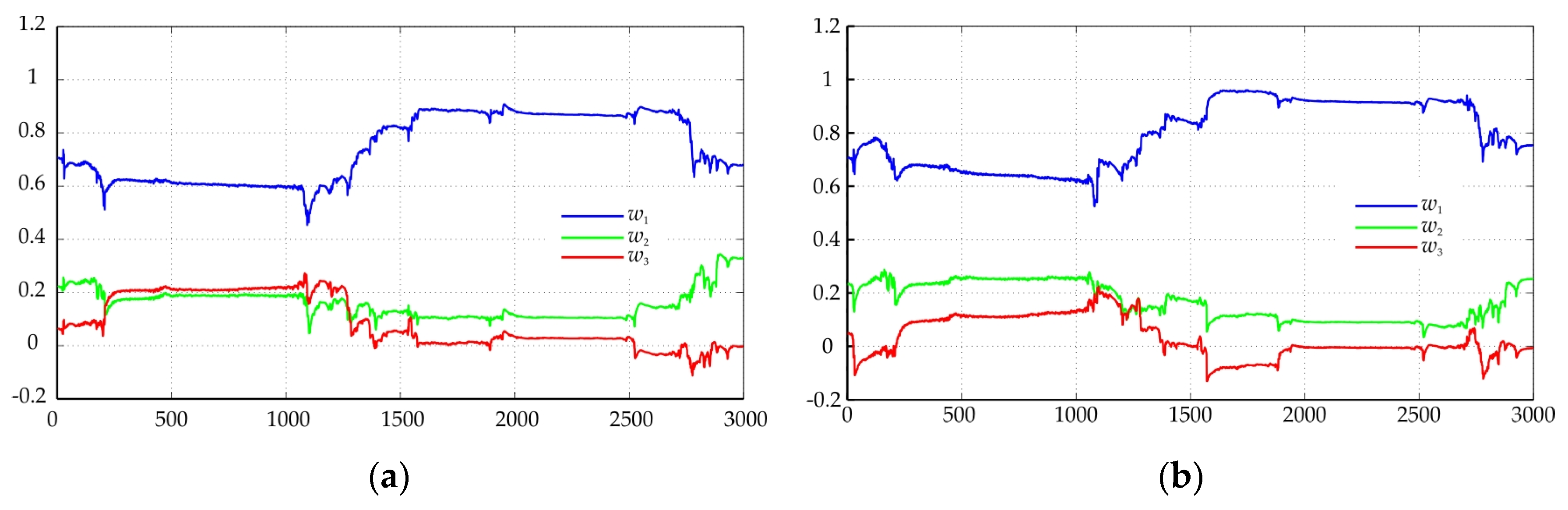
Figure 4.
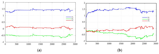
Adaptive coefficients at Trace 1: (a) 8 GHz; (b) 18 GHz.
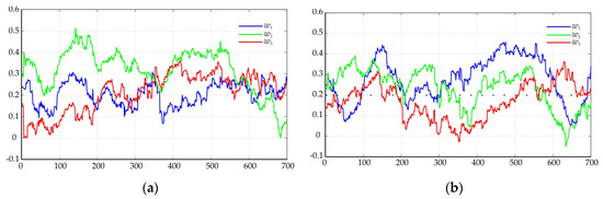
Figure 5.
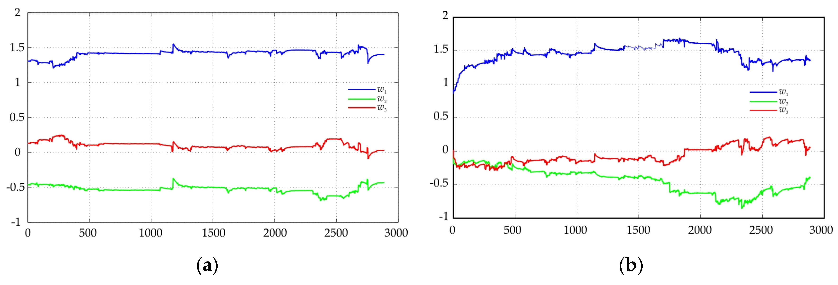
Adaptive coefficients at Trace 2: (a) horizontal polarization; (b) vertical polarization.
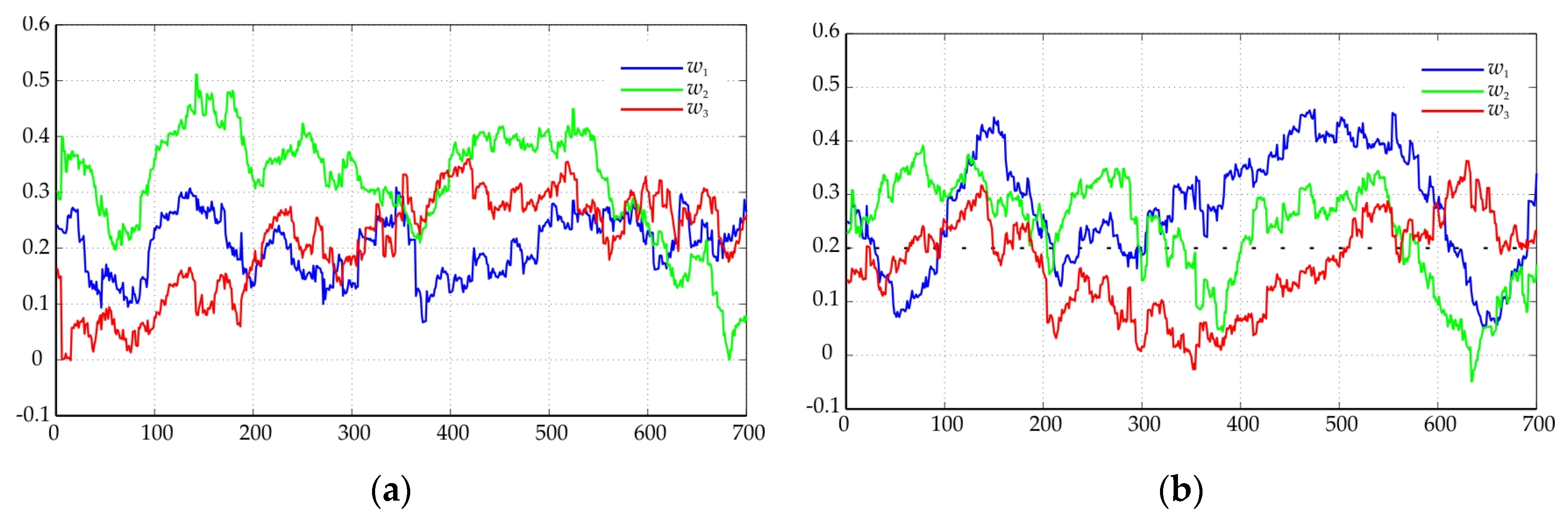
Figure 6.
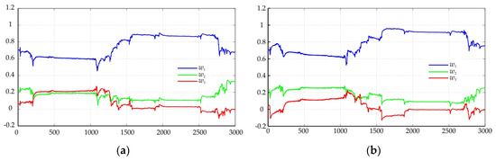
Dynamic of adaptive coefficients at Trace 3: (a) 18 GHz; (b) 28 GHz.
The proposed model with adaptive filtering of the coefficients allows a better description of the real data.
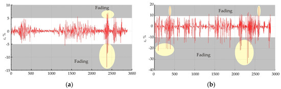
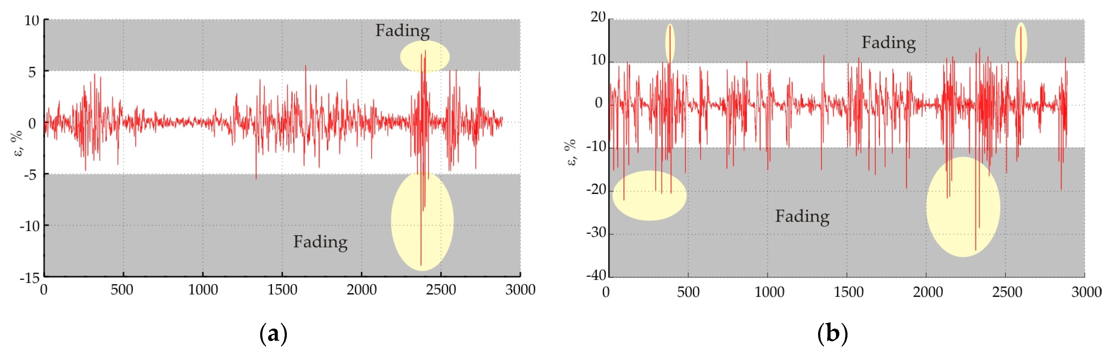
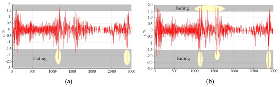
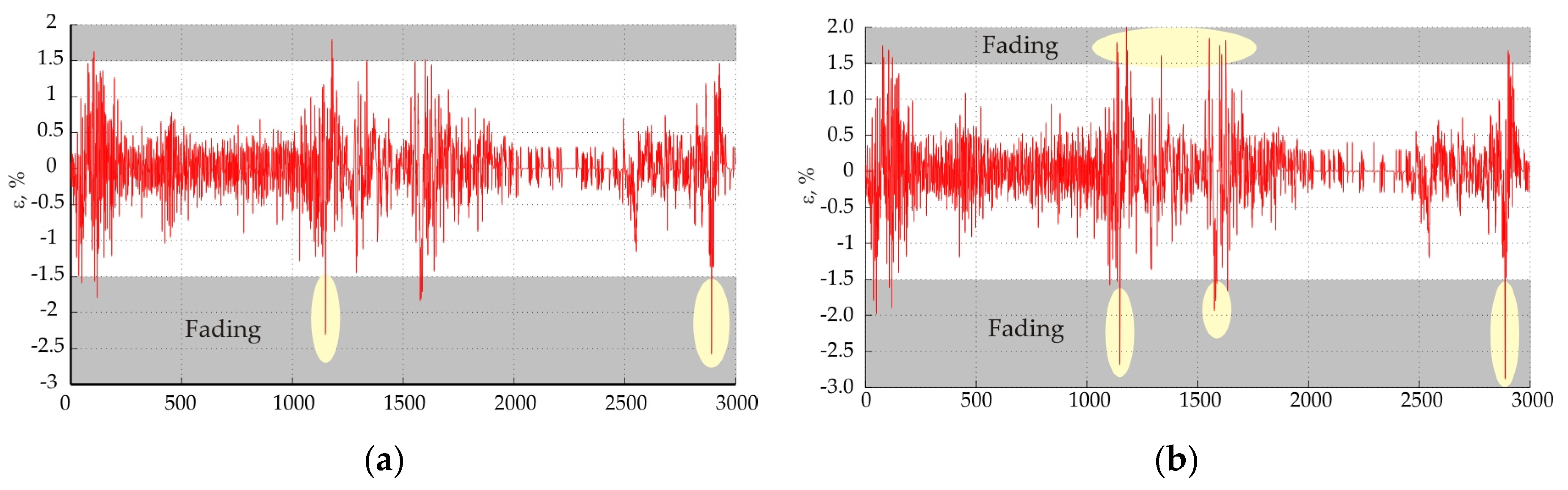
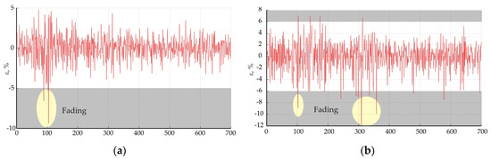
Figure 7, Figure 8 and Figure 9 show the values in the magnitude of the residuals. Areas marked with ellipses indicate the fading of the signal.
Figure 7.
Dynamics of errors on Dospat—Sarnitsa radio link: (a) at 8 GHz; (b) at 18 GHz.
Figure 8.
Simulated data of radio link Opan—Vasil Levski: (a) horizontal polarization; (b) vertical polarization.
Figure 9.
Dynamics of errors at trace Dyuni—St. Toma: (a) at 18 GHz; (b) at 28 GHz.
The error at the moment t is defined by
Substituting Equation (3) into Equation (4) for the residual sum of squares yields
Therefore, the square of the error is a function of the squared sum of the weighting coefficients. The geometric interpretation of (5) in the three-dimensional space represents a parabolic cylinder, with a certain combination of the values of the weighting coefficients . To minimize the error, the method of the fastest descent is used [8,9]. The direction of the search for the optimum is determined by
where is the gradient vector;
Therefore
where is the vector of observations.
The new weight coefficients are obtained by
where is the vector of new weight coefficients; is the vector of old weight coefficients; and k is the gradient step, as
where µ is the coefficient determining the response of the model and is called the adaptation parameter.
The optimal value of µ provides a minimum of the root mean square error of the residuals. The procedure for obtaining it is called “training” of the adaptive filter. According to the described model with adaptive filtration of the coefficients of the mathematical model, a MATLAB computer program was developed [10]. The adaptation of the mathematical model is expressed by the change in the values of the coefficients at each tact of discretization of the process.
The analysis of the residuals shows that error levels greater than ±5% correspond to the presence of fading for all three investigated traces. This corresponds to standardized levels of the residuals outside the interval probability γ < 0.05. If the level of the residuals is different from the accepted confidence probability of 95%, it can be judged as abnormal deviations which correspond to the presence of fading.
4. Conclusions
The signal levels for three radio relay routes were investigated and the characteristic conditions under which fading was observed were evaluated. On this basis, a mathematical model with adaptive filtration of the coefficients was developed in the MatLab environment. The comparison between the measured and modeled values proves the workability of the proposed model, based on which it is suggested that the size of the fragments serves as a criterion for the presence of fading along a radio relay route. For the investigated routes, a deviation of the residuals above ±5% can be assumed to be the presence of fading along the route, leading to loss of information and interruption of radio transmission.
It is appropriate to investigate whether the proposed approach is also applicable to other routes built in different geographical locations and terrains, with different carrier frequencies and different data transmission technologies.
Author Contributions
Conceptualization, T.I. and I.S.; methodology, T.I., I.S. and G.M.; software, T.I., I.S. and A.F.; validation, all; formal analysis, all; investigation, all; writing—original draft preparation, all; writing—review and editing, T.I., I.S. and G.M.; visualization, T.I., I.S. and G.M.; contributed to the interpretation of the results, M.S.P. and A.F. All authors have read and agreed to the published version of the manuscript.
Funding
This work is also partially supported by the EC Project 2020-1-PL01-KA226-HE-096196, project title: “Holistic approach towards problem-based ICT education based on international cooperation in pandemic conditions”.
Institutional Review Board Statement
Not applicable.
Informed Consent Statement
Not applicable.
Data Availability Statement
Data are obtained in the article.
Conflicts of Interest
The authors declare no conflict of interest.
References
- Sadinov, S.M.; Angelov, K.K.; Kogias, P.G.; Malamatoudis, M.N. Approach for MIMO Wireless Channel Modelling and System Characterization for an Indoor Environment. In Proceedings of the National Conference with International Participation (TELECOM), Sofia, Bulgaria, 30–31 October 2019; pp. 54–57. [Google Scholar] [CrossRef]
- Haka, A.; Vasilev, R.; Aleksieva, V.; Valchanov, H. Simulation Framework for Building of 6LoWPAN Network. In Proceedings of the 2019 16th Conference on Electrical Machines, Drives and Power Systems (ELMA), Varna, Bulgaria, 6–8 June 2019; pp. 1–5. [Google Scholar] [CrossRef]
- Lemeshko, O.; Lebedenko, T.; Al-Dulaimi, A. Improvement of Method of Balanced Queue Management on Routers Interfaces of Telecommunication Networks. In Proceedings of the 3rd International Conference on Advanced Information and Communications Technologies (AICT), Lviv, Ukraine, 2–6 July 2019; pp. 170–175. [Google Scholar] [CrossRef]
- Sadinov, S.; Kogias, P.; Angelov, K.; Malamatoudis, M.; Aleksandrov, A. The Impact of Channel Correlation on the System Performance and Quality of Service in 5G Networks. In Proceedings of the 7th International Conference on Energy Efficiency and Agricultural Engineering (EE&AE), Ruse, Bulgaria, 12–14 November 2020; pp. 1–4. [Google Scholar] [CrossRef]
- Kostadinova, S.; Markova, V.; Kostov, N.; Balabanova, I.; Georgiev, G. Latency Analysis for 5G Optical Transport Network. In Proceedings of the International Conference on Biomedical Innovations and Applications (BIA), Varna, Bulgaria, 2–4 June 2022; pp. 9–12. [Google Scholar] [CrossRef]
- Liu, X.; Chen, M.; Jiang, P.; Wang, J. Research and implementation of high data rate full digital XPIC technique. In Proceedings of the 15th International Conference on Optical Communications and Networks (ICOCN), Hangzhou, China, 24–27 September 2016; pp. 1–3. [Google Scholar] [CrossRef]
- Doubling Capacity in Wireless Channels; Provigent Inc.: Los Altos, CA, USA, November 2004; Available online: https://vdocuments.mx/xpic-tutorial.html?page=3 (accessed on 15 February 2023).
- Rencher, A.C. Methods of Multivariate Analysis; John Willey and Sons: Hoboken, NJ, USA, 2002. [Google Scholar]
- Salvatore, D.; Reagle, D. Theory and Problems of Statistics and Econometrics; McGraw Hill: New York, NY, USA, 2001. [Google Scholar]
- Eshkabilov, S. Beginning MATLAB and Simulink; Apress: New York, NY, USA, 2022. [Google Scholar]


Disclaimer/Publisher’s Note: The statements, opinions and data contained in all publications are solely those of the individual author(s) and contributor(s) and not of MDPI and/or the editor(s). MDPI and/or the editor(s) disclaim responsibility for any injury to people or property resulting from any ideas, methods, instructions or products referred to in the content. |
© 2023 by the authors. Licensee MDPI, Basel, Switzerland. This article is an open access article distributed under the terms and conditions of the Creative Commons Attribution (CC BY) license (https://creativecommons.org/licenses/by/4.0/).